Synchronous and Asynchronous Mott Transitions in Topological Insulator Ribbons

Abstract

We address how the nature of linearly dispersing edge states of two dimensional (2D) topological insulators evolves with increasing electron-electron correlation engendered by a Hubbard like on-site repulsion $U$ in finite ribbons of two models of topological band insulators. Using an inhomogeneous cluster slave rotor mean-field method developed here, we show that electronic correlations drive the topologically nontrivial phase into a Mott insulating phase via two different routes. In a synchronous transition, the entire ribbon attains a Mott insulating state at one critical $U$ that depends weakly on the width of the ribbon. In the second, asynchronous route, Mott localization first occurs on the edge layers at a smaller critical value of electronic interaction which then propagates into the bulk as $U$ is further increased until all layers of the ribbon become Mott localized. We show that the kind of Mott transition that takes place is determined by certain properties of the linearly dispersing edge states which characterize the topological resilience to Mott localization.

Topological insulators (TI) are a new quantum phase of matter distinguished by a nontrivial topology of their electronic stateKane and Mele (2005a, b); Bernevig et al. (2006); Bernevig and Zhang (2006); König et al. (2008); Moore (2010); Hasan and Kane (2010). The TI phase has been predicted and discovered in numerous compounds starting from the two-dimensional quantum spin hall (QSH) systemsBernevig et al. (2006); Bernevig and Zhang (2006) to various three-dimensional materialsHsieh et al. (2008); Hor et al. (2009); Hsieh et al. (2009a); Chen et al. (2009); Hsieh et al. (2009b). While the search is on for new materials with exotic topological characterChadov et al. (2010); Lin et al. (2010), the phenomenon presents opportunities to unravel new physics.

While the essential features of topological insulators (TI) are manifestations of one-electron physics, there is intense interest to explore the effect of electronic correlation and disorder on the topological phasePesin and Balents (2010); Rachel and Hur (2010); Varney et al. (2010); Yu et al. (2011); He et al. (2011); Yamaji and Imada (2011); Li et al. (2009). In TIs, strong spin-orbit coupling (SOC) leads to a time-reversal invariant band structure with a bulk charge gap and gapless edge modes which show Dirac like linear dispersion with a characteristic velocityHasan and Kane (2010). The gapless edge states are immune to weak perturbations (disorder/interactions) that are time reversal symmetric. A natural question that arises is regarding the fate of the Dirac dispersion with increasing electronic interactions/correlation. The system is expected to evolve to a Mott insulating state with increasing local repulsion characterized by a scale $U$. What is the mechanisim of such a Mott transition, in particular, does the edge mode velocity renormalize to zero, in an analogous fashion as the Brinkman-RiceBrinkman and Rice (1970) mechanisim of a diverging effective mass in the Hubbard model? Previous worksPesin and Balents (2010); Rachel and Hur (2010); Varney et al. (2010); Yu et al. (2011); He et al. (2011); Yamaji and Imada (2011) which addressed similar issues revealed that the gapless surface states do survive weak to moderate correlation while under stronger correlations the TI phase evolves into various insulating phases e.g., a spin liquid phase with gapped charge spectrum but gapless surface spinon excitation or a bulk antiferromagnetic insulator etc.

Of particular interest is the role of the local repulsion $U$ on the nature of electronic states in finite systems of TIs with terminating edges (we focus on 2D in this paper), such as, for example, a ribbon which is long along the $x$-direction but of finite width $L$ along the $y$-direction. The question of how interaction affects differentially the gapless edge states and the gapped bulk states existing simultaneously in such system of TIs with finite boundaries is unexplored hitherto. Such a study requires a detailed treatment that captures inhomogeneous nature of the electronic state due to the lack of translational symmetry perpendicular to the boundaries. This, along with the necessity to tackle strong interactions makes the problem difficult, even prohibitively expensive, to treat with accurate methods such as exact numerical diagonalization Varney et al. (2010). Here we study interaction effects in TI ribbons by employing an inhomogeneous cluster slave rotor mean-field (SRMF) method(Florens and Georges, 2002, 2004; Zhao and Paramekanti, 2007) which is known to provide a correct qualitative description of the Mott physicsZhao and Paramekanti (2007); Pesin and Balents (2010) while allowing for the treatment of large system sizes. The effect of local interaction is captured by introducing a Hubbard like on-site repulsion ($U$) into two well known models of 2D TIs - the Kane-Mele (KM)Kane and Mele (2005a, b) and Bernevig-Hughes-Zhang (BHZ)Bernevig et al. (2006) models. Our focus is on the dynamics in the charge sector and the concomitant Mott localization engendered by increasing $U$, following the spirit of ref. Brinkman and Rice (1970).

The highlights of the study are the following. With increasing $U$, a finite ribbon of TI attains the Mott insulating state in two distinct ways. First, in the synchronous transition, charge fluctuations vanish simultaneously on all layers (with different $y$-coordinates) of the ribbon at a critical $U_{C}$ that depends on the ribbon width $L$. The second route to the Mott state is via an asynchronous transition. Here, the charge fluctuations at the edge layers vanish at a critical $U_{E}$ which is independent of $L$. With further increase in $U$, successive layers become Mott localized until at an $L$ dependent $U_{C}$ the entire ribbon is Mott insulating. A remarkable feature here is the simultaneous realization of two phases in the ribbon – the Mott insulating (topologically trivial) state in outer layers and topologically non-trivial state in inner layers for $U_{E}<U<U_{C}$. This results in gapless modes in the bulk layers that are at the boundary between the Mott insulating and topologically non-trivial regions. We discuss the physics underlying these results later in the paper.

TI models: We briefly describe the two models for topological insulators that we study here. The KM modelKane and Mele (2005a, b) describes electrons hopping on a honeycomb lattice,

$${\cal H}_{K}= -t\sum_{\langle i,j\rangle\sigma}c_{i\sigma}^{{\dagger}}c_{j\sigma}+i\lambda\sum_{\langle\langle i,j\rangle\rangle}\sum_{\sigma\sigma^{\prime}}\nu_{ij}\tau^{z}_{\sigma\sigma^{\prime}}c_{i\sigma}^{{\dagger}}c_{j\sigma^{\prime}}$$ (1)

where $t$ is the nearest neighbor, $\langle i,j\rangle$ hopping amplitude and $\lambda$ is spin-orbit coupling strength. $\langle\langle i,j\rangle\rangle$ denote next nearest neighbor sites. $\tau^{z}$ is $z$-Pauli spin matrix and $\nu_{ij}=\pm 1$ depending on the orientation of the hopKane and Mele (2005a). For $\lambda\neq 0$, the resulting dispersion has non-trivial topology. The BHZ modelBernevig et al. (2006) defined on a square lattice with four spin-orbit coupled atomic orbitals, e.g., $\left\lvert s\uparrow\right\rangle$, $\left\lvert p\uparrow\right\rangle\equiv\left\lvert\left(p_{y}+ip_{x}\right)\uparrow\right\rangle$, $\left\lvert s\downarrow\right\rangle$, and $\left\lvert p\downarrow\right\rangle\equiv\left\lvert\left(p_{y}-ip_{x}\right)\downarrow\right\rangle$ is,

$${\cal H}_{B}=\sum_{i\alpha\sigma}\epsilon_{\alpha}c_{i\alpha\sigma}^{{\dagger}}c_{i\alpha\sigma}-\sum_{i\bm{\delta}\alpha\beta\sigma}t_{\bm{\delta}\sigma,\alpha\beta}c_{i\alpha\sigma}^{{\dagger}}c_{i+\bm{\delta}\beta\sigma}$$ (2)

where $\alpha,\beta=s,p$ and $\sigma=\uparrow,\downarrow$. $\epsilon_{\alpha}$ is the energy of the spin-orbit coupled orbital $\left\lvert\alpha\sigma\right\rangle$ and $\bm{\delta}$ denote a nearest neighbor vector. The hopping matrix elements $t_{\bm{\delta}\sigma,\alpha\beta}$ in the $\left\lvert s\sigma\right\rangle$, $\left\lvert p\sigma\right\rangle$ basis is given by (see also Fu and Kane (2007)),

$$t_{\pm\hat{x}\sigma}=\begin{pmatrix}t_{ss}&\pm\sigma\frac{it_{sp}}{\sqrt{2}}\\ \pm\sigma\frac{it_{sp}}{\sqrt{2}}&-t_{pp}\\ \end{pmatrix},\;\;t_{\pm\hat{y}\sigma}=\begin{pmatrix}t_{ss}&\pm\frac{t_{sp}}{\sqrt{2}}\\ \mp\frac{t_{sp}}{\sqrt{2}}&-t_{pp}\\ \end{pmatrix}$$ (3)

where $t_{ss}$, $t_{sp}$, $t_{pp}$ are overlap integrals and $\sigma$ takes values $+1$ ($-1$) for spin $\uparrow$ ($\downarrow$). We set $t_{ss}=t_{pp}=t$ and $t_{sp}/\sqrt{2}=v/2$, and define $\epsilon_{0}$ such that $\epsilon_{s}=-(\epsilon_{0}-4t)$ and $\epsilon_{p}=(\epsilon_{0}-4t)$. Thus we are left with three parameters for the model – $t$, $v$ and $\epsilon_{0}$. The model shows inverted band structure and hence the topological phase for $0<\epsilon_{0}<8t$.

Interactions: We introduce electron interaction via an on site Hubbard repulsion,

$${\cal H}_{U}=\frac{U}{2}\sum_{i}n_{i}(n_{i}-1)$$ (4)

to the two models in Eq. (1) and (2) where $n_{i}$ is the electron number operator. For the KM model $n_{i}=\sum_{\sigma}c_{i\sigma}^{{\dagger}}c_{i\sigma}$, while for the BHZ it is $n_{i}=\sum_{\alpha\sigma}c_{i\alpha\sigma}^{{\dagger}}c_{i\alpha\sigma}$,

Inhomogeneous SRMF Formulation: We now outline the inhomogeneous cluster SRMF formulation developed here to study the above two interacting models for lattices with ribbon geometry. In the usual slave rotor (SR) formulation(Florens and Georges, 2002, 2004; Zhao and Paramekanti, 2007), the electron operator is expressed as a product of a fermionic spinon ($f$) which carries the spin and a bosonic rotor $(\theta)$ which carries the charge. One writes $c_{i\alpha\sigma}^{{\dagger}}=f_{i\alpha\sigma}^{{\dagger}}e^{-i\theta_{i}}$ subject to the constraints, $\sum_{\alpha\sigma}n_{i\alpha\sigma}^{f}+n_{i}^{\theta}=1$ and $\sum_{\sigma}n_{i\sigma}^{e}=\sum_{\alpha\sigma}n_{i\alpha\sigma}^{f}$, where $f^{{\dagger}}_{i\alpha\sigma}$ ($e^{-i\theta_{i}}$) is the spinon creation (rotor annihilation) operator. The resulting Hamiltonian (${\cal H}_{SR}$) in terms of the auxiliary operators is then mean-field decoupled as follows. Positing the ground state of ${\cal H}_{SR}$ to be the direct product of the spinon and rotor ground states, $\left\lvert\Psi\right\rangle=\left\lvert\Psi_{f}\right\rangle\left\lvert\Psi_{\theta}\right\rangle$, one defines effective spinon and rotor Hamiltonians as ${\cal H}^{f}=\left\langle\Psi_{\theta}\right\rvert{\cal H}^{SR}\left\lvert\Psi_{\theta}\right\rangle$ and ${\cal H}^{\theta}=\left\langle\Psi_{f}\right\rvert{\cal H}^{SR}\left\lvert\Psi_{f}\right\rangle$, respectively. For the BHZ model, this gives

$${\cal H}^{f}_{B}= \sum_{i\alpha\sigma}(\epsilon_{\alpha}-\mu_{f})f_{i\alpha\sigma}^{{\dagger}}f_{i\alpha\sigma}-\sum_{i\bm{\delta}\alpha\beta\sigma}t^{f}f_{i\alpha\sigma}^{{\dagger}}f_{i+\bm{\delta}\beta\sigma}$$ (5)

$${\cal H}^{\theta}_{B}= -\sum_{i\bm{\delta}\alpha\beta\sigma}t^{\theta}e^{-i\theta_{i}}e^{i\theta_{i+\bm{\delta}}}+\frac{U}{2}\sum_{i}\left(n_{i}^{\theta}-\mu_{\theta}\right)n_{i}^{\theta}$$ (6)

where chemical potentials are introduced to control the mean particle density. The effective hopping parameters $t^{f}$ and $t^{\theta}$ are given by $t^{f}_{i\bm{\delta}\sigma,\alpha\beta}=t_{\bm{\delta}\sigma,\alpha\beta}B_{i,i+\bm{\delta}}$ and $t^{\theta}_{i\bm{\delta}\sigma,\alpha\beta}=t_{\bm{\delta}\sigma,\alpha\beta}\chi_{i\alpha,i+\bm{\delta}\beta}^{\sigma}$, where $B_{ij}=\left\langle\Psi_{\theta}\right\rvert e^{-i(\theta_{i}-\theta_{j})}\left\lvert\Psi_{\theta}\right\rangle$ and $\chi_{i\alpha,j\beta}^{\sigma}=\left\langle\Psi_{f}\right\rvert f^{{\dagger}}_{i\alpha\sigma}f_{j\beta\sigma}\left\lvert\Psi_{f}\right\rangle$ (analogous expressions are used for the KM model). The resulting spinon and rotor Hamiltonians are solved self consistently to obtain the ground state. A key point to be noted here is that the $B$s and $\chi$s are bond dependent in a ribbon, i. e., they are inhomogeneous. The spinon Hamiltonian is quadratic albeit with inhomogeneous renormalized hopping parameters and hence can be diagonalized numerically The rotor problem, however, is non-quadratic and a full numerical solution is still prohibitive, and additional approximations such as cluster mean field method have to be adopted. In conventional cluster mean-field methodZhao and Paramekanti (2007), one considers a small cluster of sites where the rotor Hamiltonian is treated exactly. Terms connecting the sites inside the cluster to sites outside (bath) are decoupled by using, $\Phi_{i}=\langle e^{i\theta_{i}}\rangle$ where $\Phi_{i}$ is a site-dependent mean-field parameter also to be obtained self-consistently. This quantity plays an important role in that it signifies charge fluctuation at the site $i$. A nonzero $\Phi_{i}$ implies charge fluctuation whereas vanishing of $\Phi_{i}$ implies a “local” Mott insulating phase.

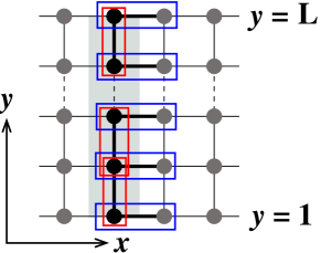
Figure 1: Inhomogeneous cluster mean-field method. Each unique bond in the strip which is treated as a distinct cluster is shown enclosed by a rectangle. The shaded region represents a unit cell of the strip.

To take into account the inhomogeneity introduced by the lost translational symmetry in the $y$-direction, we first express the ${\cal H}^{\theta}_{B}$ as a sum of bond terms, i.e., as ${\cal H}^{\theta}_{B}=\sum_{b_{ij}}h^{\theta}_{ij}$. Now we treat the bonds (such as those shown in Fig. 1) one at a time as our cluster and the rest as the bath and obtain a mean-field two-site cluster Hamiltonian for each bond. Each of the bond problem then solved to obtain a self-consistent set of solutions for $\{\Phi_{y}\},\;y=1,\ldots,L$. We treat all the unique bonds (coloured boxes in Fig. 1) in the super-cell (indicated by the shaded region in Fig. 1) utilizing the translational symmetry in the $x$-direction. The above inhomogeneous calculation becomes numerically expensive (for typical width of $L=100$ considered here) as it involves diagonalization of a large number of rotor Hamiltonians in each iteration of the self consistency loop.

We also obtain the bulk phase diagram (lattice with no boundaries) where the parameters $\Phi$, $B$, $\chi$ are all site independent (homogeneous). For this, it suffices to solve the rotor mean-field Hamiltonian only for a single cluster. In the results discussed below all energies are measured in units of appropriate $t$ both for the KM and BHZ models.

   

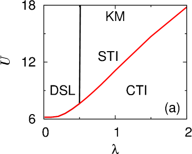
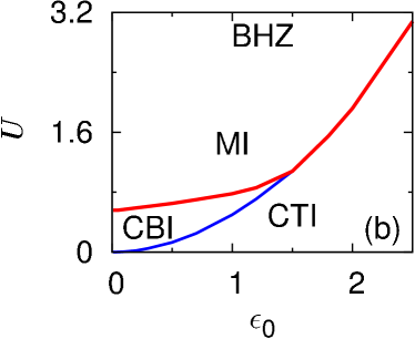
Figure 2: Bulk phase diagram - (a) KM model: There are three phases:- Correlated Topological Insulator (CTI), DSL (Dirac Spin Liquid), STI (Spinon Topological Insulator) phases. DSL/STI phases are Mott insulating. (b) BHZ model: There are three phases:- CTI, Correlated Band Insulator (CBI) and MI (Mott insulator).

KM Model Results: We first discuss the bulk phase diagram of the KM model (see Fig. 2(a)) obtained within our formulation. For any given $\lambda$ there is a critical $U_{B}$ such for $U>U_{B}$ a Mott insulating state is obtained. For $U<U_{B}$ (region below the red line Fig. 2(a)), there are local charge fluctuations even though there is a charge/spin gap, and the spinon dispersion is topologically nontrivial – we call this state a correlated topological insulator (CTI). There are two regimes of $\lambda$ for which the Hubbard interaction produces different types of Mott states. For $\lambda<\lambda_{c}=\frac{1}{2}$, the Mott state is a Dirac spin liquid (DSL), i. e., a state with no charge fluctuations and a gapless spinon dispersion similar to that of graphene. In this regime effective $\lambda$ for the spinon hopping renormalizes to zero. For $\lambda>\lambda_{c}$, the Mott state has a gapped topologically non-trivial spinon spectrum (spinon topological insulator (STI)) - the state has local spin fluctuations but no charge fluctuations. All the boundaries in Fig. 2 correspond to second order transitions in that $\Phi$ goes to zero continuously with increasing $U$.

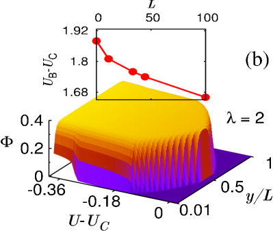
Figure 3: Mott transition in KM ribbons of width $L=50$. in the two different regimes of $\lambda$. (a) Synchronous Mott transition obtained for $\lambda=0.1$ where the entire ribbon becomes Mott insulating at a critical value of $U_{C}$. The bulk value of critical Hubbard interaction is $U_{B}=6.19$. (b) Asynchronous Mott transition for $\lambda=2$ ($U_{B}=17.8$). The edge sites go Mott insulating at $U_{E}=15.8$, followed by successive layers becoming Mott insulating with increasing $U$ until the ribbon becomes fully Mott insulating at $U=U_{C}$. Dependence of $U_{C}$ on the width $L$ of the ribbon is shown in the upper insets in both cases.

We now turn to zigzag edge terminated ribbons of finite width. Fig. 3 shows plot of $\Phi_{y}$ as a function of $U$ and $y$ for two values of $\lambda$, e.g., $0.1$ and $2$. For $\lambda=0.1<\lambda_{c}$, the bulk value of the critical Hubbard interaction is $U_{B}=6.19$. As shown in Fig. 3(a), for this value of $\lambda$, the Mott transition of the ribbons occurs in a “synchronous” fashion, i. e., the charge fluctuations vanish throughout the strip at a critical value of $U_{C}$. $U_{C}$ is quite close to $U_{B}$ and the difference between $U_{B}$ and $U_{C}$ falls with increasing width of the ribbon (see inset in Fig. 3(a)).

For the value of $\lambda=2>\lambda_{c}$ we find completely different physics. In this case, the edge sites (see Fig. 3(b)) undergo a local Mott transition at a value of $U_{E}=15.8$ which is significantly smaller than the bulk value for the Mott transition $U_{B}=17.8$ while the sites in the bulk continue to enjoy charge fluctuations. Most interestingly, this critical value $U_{E}$ does not depend on the with $L$ of the ribbon over the range of ribbon widths $L=10$ to $100$ studied in this work. Further increase of $U$ above $U_{E}$ results in successive layers attaining the Mott insulating state (Fig. 3(b)) – a phenomenon we call “asynchronous” Mott transition. The process of asynchronous Mott transition continues until a width dependent critical $U_{C}$ is attained. $U_{C}$ is always less than $U_{B}$ (see inset of Fig. 3(b)) and $U_{C}\rightarrow U_{B}$ as $L$ becomes larger.

The key point to be noted is that the nature of the Mott transition in KM ribbons is determined by $\lambda$. For all $\lambda<\lambda_{c}$ we find synchronous Mott transition, while the second regime $\lambda>\lambda_{c}$, asynchronous behaviour is obtained.

  

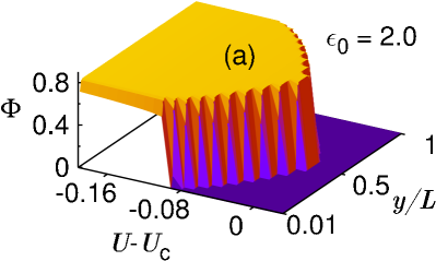
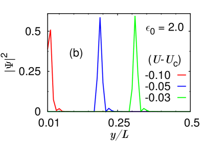
Figure 4: (a) Asynchronous Mott transition in a BHZ ribbon with $L=100$. (b) Wave function of mode that appears at the MI – CTI interface in the asynchronous Mott transition. For $U\leq U_{E}$, the mode is localized at the edge of the sample (red curve). With increasing $U>U_{E}$ the outer layers become Mott insulating and the interface modes appear in the inside layers of the ribbon.

BHZ Model Results: The results discussed here are for $t=v=1$. Fig. 2(b) shows the bulk phase diagram of the BHZ model. There are again two regimes of the topological parameter. For $\epsilon_{0}<3/2$, there are two transitions with increasing $U$. In this regime first transition is at $U_{A}$, where the spinon dispersion becomes topologically trivial, but the system is still not Mott insulating, i. e., the system effectively is a correlated band insulator (CBI). At a larger critical value $U_{B}$, the CBI state undergoes a Mott transition and obtains paramagnetic Mott insulator. The spinon dispersion renormalizes to zero. When $\epsilon_{0}>3/2$, the CTI phase gives way to the MI phase without the intervening CBI phase. The Mott transition in this case is a first order transition (unlike in the KM case).

Fig. 4(a) shows asynchronous Mott transition in a BHZ ribbon for $\epsilon_{0}=2$. In fact, all BHZ ribbons that we have studied over a range of $\epsilon_{0}$ and widths $L$ undergo asynchronous transitions. All other qualitative features of the transition are similar to that of the KM model. An interesting aspect is that in both models, the asynchronous Mott transition leads to a state with trivial topology. Thus between $U_{E}$ and $U_{C}$ the ribbon consists of two regions, one adjoining the edges that is Mott insulating and topologically trivial, while the center portion continues to be a CTI endowed with a non-trivial topology. Thus one expects interface modes to appear at the layer that separates the two regions which is now in the bulk of the ribbon and to evolve further into the bulk as $U$ increases from $U_{E}$ to $U_{C}$. Indeed, we do find such spinon modes as shown for the BHZ model in Fig. 4(b). KM model also has similar physics in the asynchronous regime.

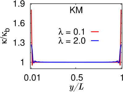
Figure 5: Local site compressibility $\kappa(y)/\kappa_{B}$ for the KM model.

Why are there two types of transitions and what governs this? The nature of the transition is governed by the local nature of the topological edge states. The quantity $\kappa(y)=\lim_{\beta\rightarrow\infty}\int_{0}^{\beta}d\tau\langle n_{y}(\tau)n_{y}(0)\rangle-\langle n_{y}(0)\rangle^{2}$, where $\beta$ is inverse temperature, calculated using the non-interacting Hamiltonian is a measure of the local compressibility of a site in a layer at a given $y$. If the edge states brought about by the topological dispersion results in a large compressibility compared to the bulk, then the edge sites resist Mott localization – topological resilience to Mott localization – since much kinetic energy is lost in localizing carriers at the edges. Indeed for the KM model, the velocity of edge states for $\lambda\ll\lambda_{c}$ is $6\lambda$ while for $\lambda=2$ the edge state velocity is $0.75\lambda$. This is reflected in a large site compressibility at the edges compared to the bulk value ($\kappa_{B}$) for $\lambda=0.1$ (see Fig. 5). For highly compressible edges, Mott transition of the ribbons occurs at value of $U$ close to that of the bulk value and occurs in a synchronous fashion. In the other limit where the edge site compressibility is comparable or lower to that of the bulk (as is the case for $\lambda=2$ in KM, and for the BHZ model), Hubbard energy dominates since there is no significant kinetic energy to be gained and Mott localization occurs at value of $U$ significantly lower than the bulk. The kinetic energy of the bulk spinon modes comes to play; these modes prevent the synchronous Mott transition and rendering it asynchronous. Our arguments, if applied, to the usual one band square lattice half-filled Hubbard model (no edge states) will predict an asynchronous transition for finite ribbons – indeed we do find this in our SRMFT simulations of such systems.

Interestingly, for the synchronous Mott transition the spinon edge mode velocity is continuously renormalized to lower values as $U$ approaches $U_{C}$. In the asynchronous case, the edge modes “switch layers” and eventually vanish at $U_{C}$. This provides a clear physical picture of the nature of the Mott transition in finite ribbons of TIs. Another important outcome of this study pertains to the use of surface probes to investigate the electronic state correlated materials (particularly topological insulators). A key point to be borne in mind is that surface may show insulating character while the bulk may still be locally compressible.

VBS thanks DST (Ramanujan grant) and DAE (SRC grant), HRK thanks DST (Bose grant) for support.

References

- Kane and Mele (2005a) C. L. Kane and E. J. Mele, Phys. Rev. Lett. 95, 146802 (2005a).
- Kane and Mele (2005b) C. L. Kane and E. J. Mele, Phys. Rev. Lett. 95, 226801 (2005b).
- Bernevig et al. (2006) B. A. Bernevig, T. L. Hughes, and S.-C. Zhang, Science 314, 1757 (2006).
- Bernevig and Zhang (2006) B. A. Bernevig and S.-C. Zhang, Phys. Rev. Lett. 96, 106802 (2006).
- König et al. (2008) M. König, H. Buhmann, L. W. Molenkamp, T. Hughes, C.-X. Liu, X.-L. Qi, and S.-C. Zhang, J. Phys. Soc. Jpn. 77, 031007 (2008).
- Moore (2010) J. E. Moore, Nature 464, 194 (2010).
- Hasan and Kane (2010) M. Z. Hasan and C. L. Kane, Rev. Mod. Phys. 82, 3045 (2010).
- Hsieh et al. (2008) D. Hsieh, D. Qian, L. Wray, Y. Xia, Y. S. Hor, R. J. Cava, and M. Z. Hasan, Nature 452, 970 (2008).
- Hor et al. (2009) Y. S. Hor, A. Richardella, P. Roushan, Y. Xia, J. G. Checkelsky, A. Yazdani, M. Z. Hasan, N. P. Ong, and R. J. Cava, Phys. Rev. B 79, 195208 (2009).
- Hsieh et al. (2009a) D. Hsieh, Y. Xia, D. Qian, L. Wray, J. H. Dil, F. Meier, J. Osterwalder, L. Patthey, J. G. Checkelsky, N. P. Ong, A. V. Fedorov, H. Lin, A. Bansil, D. Grauer, Y. S. Hor, R. J. Cava, and M. Z. Hasan, Nature 460, 1101 (2009a).
- Chen et al. (2009) Y. L. Chen, J. G. Analytis, J.-H. Chu, Z. K. Liu, S.-K. Mo, X. L. Qi, H. J. Zhang, D. H. Lu, X. Dai, Z. Fang, S. C. Zhang, I. R. Fisher, Z. Hussain, and Z.-X. Shen, Science 325, 178 (2009).
- Hsieh et al. (2009b) D. Hsieh, Y. Xia, D. Qian, L. Wray, F. Meier, J. H. Dil, J. Osterwalder, L. Patthey, A. V. Fedorov, H. Lin, A. Bansil, D. Grauer, Y. S. Hor, R. J. Cava, and M. Z. Hasan, Phys. Rev. Lett. 103, 146401 (2009b).
- Chadov et al. (2010) S. Chadov, X. Qi, J. Kúbler, G. H. Fecher, C. Fecher, and S. C. Zhang, Nature Mat. 9, 541 (2010).
- Lin et al. (2010) H. Lin, L. A. Wray, Y. Xia, S. Xu, S. Jia, R. J. Cava, A. Bansil, and M. Z. Hasan, Nature Mat. 9, 546 (2010).
- Pesin and Balents (2010) D. Pesin and L. Balents, Nature Phys. 6, 376 (2010).
- Rachel and Hur (2010) S. Rachel and K. L. Hur, Phys. Rev. B 82, 075106 (2010).
- Varney et al. (2010) C. N. Varney, K. Sun, M. Rigol, and V. Galitski, Phys. Rev. B 82, 115125 (2010).
- Yu et al. (2011) S.-L. Yu, X. C. Xie, and J.-X. Li, Phys. Rev. Lett. 107, 010410 (2011).
- He et al. (2011) J. He, S.-P. Kou, Y. Liang, and S. Feng, Phys. Rev. B 83, 205116 (2011).
- Yamaji and Imada (2011) Y. Yamaji and M. Imada, Phys. Rev. B 83, 205122 (2011).
- Li et al. (2009) J. Li, R.-L. Chu, J. K. Jain, and S.-Q. Shen, Phys. Rev. Lett. 102, 136806 (2009).
- Brinkman and Rice (1970) W. F. Brinkman and T. M. Rice, Phys. Rev. B 2, 4302 (1970).
- Florens and Georges (2002) S. Florens and A. Georges, Phys. Rev. B 66, 165111 (2002).
- Florens and Georges (2004) S. Florens and A. Georges, Phys. Rev. B 70, 035114 (2004).
- Zhao and Paramekanti (2007) E. Zhao and A. Paramekanti, Phys. Rev. B 76, 195101 (2007).
- Fu and Kane (2007) L. Fu and C. L. Kane, Phys. Rev. B 76, 045302 (2007).
- Note (1) Since our focus is on the charge sector and the associated Mott physics in the spirit of Brinkman and Rice (1970), we keep aside the magnetic correlations which are typically introduced by adding an exchange term in the HamiltonianRachel and Hur (2010) and treating it via mean field theory.