Rupture of a Biomembrane under Dynamic Surface Tension

Abstract

How long a fluid membrane vesicle stressed with a steady ramp of micropipette last before rupture? Or conversely, how high the surface tension should be to rupture a membrane? To answer these challenging questions we have developed a theoretical framework that allows description and reproduction of Dynamic Tension Spectroscopy (DTS) observations. The kinetics of the membrane rupture under ramps of surface tension is described as a combination of initial pore formation followed by Brownian process of the pore radius crossing the time-dependent energy barrier. We present the formalism and derive (formal) analytical expression of the survival probability describing the fate of the membrane under DTS conditions. Using numerical simulations for the membrane prepared in an initial state with a given distribution of times for pore nucleation, we have studied the membrane lifetime (or inverse of rupture rate) and distribution of membrane surface tension at rupture as a function of membrane characteristics like pore nucleation rate, the energy barrier to failure and tension loading rate. It is found that simulations reproduce main features of the experimental data, particularly, the pore nucleation and pore size diffusion controlled limits of membrane rupture dynamics. This approach can also be applied to processes of permeation and pore opening in membranes (electroporation, membrane disruption by antimicrobial peptides, vesicle fusion).
PACS numbers: 05.10.Gg, 87.10.-e, 87.16.A-

I Introduction

Many aspects of biological life crucially depend on stability of cell membranes for which several properties are not understood yet. Fluid lipid bilayers are the building blocks of biological membranes. Pores in such systems play an important role in the diffusion of small molecules across biomembranes PV96 . As well pore formation is a possible mechanism for vesicle fusion SK01 . In order for any vesicle to be useful it must be relatively stable. Yet in order to undergo fusion, long-lived holes must occur during the fusion transformation. How membranes actually manage to exhibit these two conflicting properties is not completely clear, but this can likely be realized only dynamically. Dynamic properties are especially important for biological membranes, because their static characteristics describe a dead structure whereas life and biological functions are associated with molecular motions. Thus, the desire to understand the dynamics of biomembrane rupture, which is the main aim of this paper, is hardly surprising.

On a microscopic level, pores are formed owing to thermal motion of lipid molecules and, in principle, various types of pores can be distinguished. It usually is assumed that initially nucleated pores have hydrophobic edges; the so-called hydrophobic pores GL88 which are spontaneously formed in the lipid matrix. The probability for the existence of such hydrophobic pores is determined by the free energy of pore as a function of pore radius (see Sections II and III below). And, when the hydrophobic pore exceeds a critical size, a reorientation of the lipids takes place converting the pore into an hydrophilic one where the head groups form the pore walls. As discussed in TL03 , these reorientation processes can occur at the very early stages of pore formation so that nucleation is the crucial step in the rupture process. Note that thermal fluctuations can as well lead to transient unstable pores, often termed as pre-pores HU06 . In what follows, we will be interested on stable pores (i. e., a well defined density of pores which can be detected, e.g., by neutron scattering, with individual pores forming and resealing reversibly) and head group reorientation mechanisms will be disregarded. All details on hydrophobic and hydrophilic pores will be lumped into the effective model parameters like line tension, (unstressed) membrane surface tension, and pore size diffusion coefficient. Electric breakdown method provides information on pore size which can be drawn from the dependence of membrane conductivity on applied voltage GL88 , but dynamical pore characteristics can be hardly found by this technique. One of the most relevant material parameter controlling pore dynamics is membrane surface tension. Surface tension suppressing thermal fluctuations and promoting membrane adhesive properties, can induce adhesion of a membrane onto a substrate or to another membrane, and other tension induced morphological transitions including membrane rupture.

A closed vesicle without pores can survive for a very long period of time. Pores can form and grow in the fluid-lipid membrane in response to thermal fluctuations and external influences. Several innovative techniques are available for observing transient permeation and opening of pores. These include mechanical stress, strong electric fields (electroporation), optical tweezers, imploding bubbles, adhesion at a substrate, and puncturing by a sharp tip. In all instances, the resulting transient pore is usually unstable and leads to membrane rupture for some level of the surface tension. Using the rupturing of biomembranes under ramps of surface tension, the challenge of the Dynamic Tension Spectroscopy (DTS) is to identify and quantify the relevant parameters that govern the dynamics of membrane rupture and thereby characterize the membrane mechanical strength.

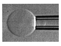
Figure 1: Image of a 20 mm bilayer vesicle aspirated in a micropipette (from Ref. EHLR03 ).

As a demonstration of the DTS technique, Evans et al. EHLR03 conducted experiments of rupturing fluid membrane vesicles with a steady ramp of micropipette suction (Fig. 1). Rupture tests on different types of giant phosphatidychlorine lipid vesicles over loading rate (tension/time) from 0.01 and up to 100 mN/m/s produce distributions of breakage tensions governed by the kinetic process of membrane failure. One might naively expect that lipid membranes to rupture at tensions close to hydrocarbon - water surface tension as lipids are held together by hydrophobic interactions. However, biomembranes rupture at much lower tension. As pointed out by Evans et al., rupture strength of a biomembrane is a dynamical property and that the level of strength depends on the time frame for breakage EHLR03 . Energy barriers along the tension driven pathway are determinants of membrane strength, and the relative heights of these barriers lead to time-dependent changes in strength. To describe dynamic tension spectra they observed, Evans et al. modeled the membrane breakage as a sequence of two successive thermally-activated transitions (dependent of loading rates) limited either by specific defect (pre-pore) formation or by passage over the cavitation barrier (or evolution to an unstable pore). Accordingly, this description was formalized into a three-state kinetic model for the membrane: the defect-free ground state, the defect or metastable state, and the ruptured membrane state EHLR03 .

Motivated by these experimental and theoretical investigations and findings, our objective in this paper is to develop a minimal theoretical framework of the DTS method to describing the kinetic process of membrane breakage. Based on the general framework of Kramers reaction rate theory Kra40 ; HTB90 , we develop in this paper a theoretical framework for DTS to describe the pore growth and membrane rupture dynamics as a Markovian stochastic process crossing a time-dependent energy barrier. As mentioned, such a theoretical approach is conceptually similar to that used by Evans et al., EHLR03 (see also, FJ03 ; BJ07 ). However, our description is more general than that presented in EHLR03 as it characterizes and describes both primary nucleation event followed by the continuous dynamics of pore growth and shrinking allowing hence easy to follow and adapt for further numerical treatments.

II Problem Formulation

In what follows, we treat the membrane as a two-dimensional continuum medium and we neglect shape fluctuations, i.e., the parameter $\delta\equiv k_{B}T/4\pi\kappa$ SA94 is small (e.g., $\delta\sim 10^{-3}$ for lipid bilayers). We will deal with thermal fluctuations not related with shape fluctuations but with the process of barrier crossing for pore formation characterized by the parameter $\varepsilon=V_{0}/k_{B}T$, where $V_{0}$ is the typical energy cost for pore formation at the critical pore radius (see Eq.(11) below). Thus, our investigations will concern the regime, $\delta\ll 10^{-1}\leq\varepsilon$.

Within the framework of the DTS, we describe the kinetic of membrane rupture as a succession of two processes: an initial pore nucleation followed by a diffusion dynamics of the pore size to membrane rupture.

II.1 Pore Formation

For simplicity, we assume that the net process of pore nucleation in a membrane can be described by an activated process following a first-order kinetics with a rate $q$, i.e., the distribution of times for the membrane to remain free of pores is given by the exponential distribution with the rate, $q$, which is a function of membrane characteristics. For the purpose of DTS, we will assume that the pore nucleation rate $q(\sigma)$ is a function of membrane surface tension $\sigma$.

II.2 Pore Diffusion

Once the pore is already formed in the membrane, the net energy $V(r)$ of such a membrane of thickness $l$ with a circular pore of radius $r$ consists of two opposed terms L75 : the surface tension $\sigma$, favoring the expansion, and the energy cost $\gamma$ of forming a pore edge (line tension), favoring the closure:

$$V(r)=2\pi\gamma\,r-\pi\sigma\,r^{2}\>.$$ (1)

Assuming that $\sigma>0$ and $\gamma>0$, and both are constant, Eq.(1) predicts that for $r<a$, where $a=\gamma/\sigma$ is the pore radius for the maximum energy $V(r)$, the radial force associated with a change in radius tends to reseal the pore, and the membrane remains stable against pore growth. On the other hand, a pore with a radius larger than the critical value $a$ will grow without bound and, ultimately, will rupture the membrane. In DTS experiments EHLR03 , the membrane is stressed such that (provided that $\gamma$ remains constant) the surface tension grows linearly with time as, $\sigma=\sigma_{0}+Ft$, where $\sigma_{0}$ is the unstressed membrane tension and $F$ is the loading rate constant. In this case, the critical radius $a(t)$ becomes a decreasing function of time and any pore initially with radius $r<a(0)$ will ultimately lead to membrane rupture at time such that $r>a(t)$ as a result of the decreasing of both the critical pore radius and associated barrier energy. Now, incorporating thermal fluctuations in this picture, one can view the rupture of the membrane as a Brownian process crossing the time-dependent energy barrier $V[a(t)]$.

To setup the equations of pore size dynamics, we consider a membrane with a pore of radius $r$ under mechanical stress that changes its surface tension. In this description model of DTS, the surface tension $\sigma$ in $V(r)$ is a linear function of time as defined above. Thus, neglecting inertial effects, the dynamics of $r$ is governed by the Langevin equation with time-dependent potential,

$$\left\{\begin{array}[]{l}\displaystyle\zeta\,\frac{dr}{dt}=-\frac{dV(r,t)}{dr}+f(t)\\ \\ \displaystyle V(r,t)=2\pi\gamma\,r-\pi\left(\sigma_{0}+Ft\right)\,r^{2}\end{array}\right.$$ (5)

where $\zeta=4\pi\eta_{m}\,l$ is the friction coefficient to radial circular fluctuations with $\eta_{m}$ the internal 2d membrane viscosity, and $f(t)$ is a Gaussian random force of zero mean with correlation function given by the fluctuation-dissipation relation, $\langle f(t)f(t^{\prime})\rangle=2\,\zeta\,{\rm k_{B}T}\,\delta(t-t^{\prime})$, with ${\rm k_{B}T}$ being the thermal energy.

II.3 Dimensionless equations

To work with dimensionless variables, we define in Table 1 scales of length, surface tension and time by $r_{0}$, $\sigma_{0}$ and $\tau$, respectively, and we consider the following transformations: $x=r/r_{0}$, $y=\sigma/\sigma_{0}$, and $t\rightarrow t/\tau$ (with $x\in[0,1]$ and $y\in[1,\infty[$) . This operation leads us to define the control parameter,

$$v=\frac{F\tau}{\sigma_{0}}\equiv\frac{\mbox{diffusing time scale}}{\mbox{surface tension time scale}}\>.$$ (6)

This parameter allows us to distinguish two regimes in the dynamics of the membrane rupture: the diffusion controlled regime when $v\ll 1$ and the drift regime for $v\gg 1$ limit. With these transformations Eq.(5) can be rewritten as,

$$\left\{\begin{array}[]{l}\displaystyle\frac{dx}{dt}=-\frac{dU(x,y)}{dx}+X(t)\\ \\ \displaystyle\frac{dy}{dt}=v\end{array}\right.$$ (10)

where $X(t)$ is a Gaussian random force of zero mean with correlation function given by, $\langle X(t)X(t^{\prime})\rangle=2\,\delta(t-t^{\prime})$, and we have defined the potential (energy landscape for DTS illustrated in Fig 2),

$$U(x|y)=\frac{\varepsilon}{2}\,\left[2x-yx^{2}\right]\>\>;\>\>\varepsilon=\frac{V(r_{0})}{\rm k_{B}T}=\frac{\pi\gamma^{2}}{\sigma_{0}{\rm k_{B}T}}\>.$$ (11)

The potential $U(x|y)$ is maximum at $x^{{\ddagger}}=1/y$ corresponding to the energy barrier $U^{{\ddagger}}=U(x^{{\ddagger}}|y)=\varepsilon/2y$. Both the position $x^{{\ddagger}}$ and height $U^{{\ddagger}}$ of the energy barrier decrease as $y$ gets larger as a result of the membrane stress.

Figure 2: Energy landscape (Eq.(11) with $\varepsilon=2$) for the Dynamic Tension Spectroscopy. Flat area $x>2/y$ corresponds to $U<0$.

Table 1: Parameters and dimensionless variables. The index ”0” denotes quantities for unstressed membrane.

Symbols	Definition
$\gamma$	line tension (energy/length)
$\sigma_{0}$	unstressed surface tension (energy/surface)
$F$	tension loading rate (energy/surface/time)
$D={\rm k_{B}T}/\zeta\,l$	pore diffusion coefficient (length2/time)
$r_{0}=\gamma/\sigma_{0}$	critical pore radius (length)
$\tau=r_{0}^{2}/D$	diffusing time scale of the critical pore (time)
$F_{0}=\sigma_{0}/\tau$	critical tension loading rate (energy/surface/time)
$q_{0}$	reduced unstressed pore nucleation rate
$x=r/r_{0}$	reduced pore radius
$y=\sigma/\sigma_{0}$	reduced membrane surface tension
$\varepsilon=\pi\gamma^{2}/\sigma_{0}{\rm k_{B}T}$	reduced energy barrier for unstressed membrane
$v=F/F_{0}$	reduced tension loading rate:$\left\{\begin{array}[]{l}\!v<1\,:\,\mbox{diffusing limit}\\ \!v>1\,:\,\mbox{drift limit}\end{array}\right.$

II.4 DTS observables

As the barrier crossing to both pore nucleation and membrane rupture are stochastic processes, both the membrane lifetime and the membrane tension at rupture are distributed. Our goal is to calculate the two quantities that characterize the kinetics of membrane rupture in DTS framework: the rate of membrane rupture and the distribution of tension at membrane rupture.

For a membrane with a pore in the absence of mechanical stress $v=0$, the distribution of tension at membrane rupture is delta function, $Q(y)=\delta(y-1)$, and the rate of membrane rupture can be obtained analytically using the first passage time approach SSS80 ; BS97 ,

$$\frac{1}{k(\varepsilon|0)}=\int_{0}^{1}\!\frac{dx}{p_{\rm eq}(x|1)}\,\left[\int_{0}^{x}\!p_{\rm eq}(z|1)\,dz\right]^{2}$$ (12)

$$= \frac{\sqrt{\pi/(2\varepsilon)}}{{\rm erfi}\left[\sqrt{\varepsilon/2}\right]}\int_{0}^{1}\!dx\,{\rm e}^{-\varepsilon(x-1)^{2}/(2)}$$

$$\times\left\{{\rm erfi}\left[\sqrt{\varepsilon/2}\right]-{\rm erfi}\left[(1-x)\sqrt{\varepsilon/2}\right]\right\}^{2}$$

in which we have assumed that the membrane system was initially prepared with the distribution $p_{\rm eq}(x|1)$, where

$$p_{\rm eq}(x|y)=\frac{{\rm e}^{-U(x|y)}}{Z(y)}\>;\>Z(y)=\int_{0}^{1/y}\!{\rm e}^{-U(x|y)}\,dx\>,$$ (13)

and $Z(y)=\displaystyle\left(\frac{\pi{\rm e}^{-\varepsilon/y}}{2\varepsilon y}\right)^{1/2}\,{\rm erfi}\left[\sqrt{\varepsilon/2y}\right]$ where ${\rm erfi}[z]={\rm erf}[iz]/i$ and ${\rm erf}[\cdots]$ is the error function.

On the other hand, for a membrane initially free of pore and for $v>0$, analytical expressions are not straightforward but the rate of membrane rupture and the distribution of tension at membrane rupture can be determined as follows. Let $S(t)$ be the survival probability that describes the fate of the membrane from the beginning of the experiment. The distribution of membrane lifetime or rupture time is given by $-dS/dt$, and the membrane rupture rate (equals to the inverse of the membrane lifetime) is obtained as,

$$\frac{1}{k(\varepsilon|v)}=\int_{0}^{\infty}\!t\left[-\frac{dS(t)}{dt}\right]\,dt=\int_{0}^{\infty}\!S(t)\,dt\>.$$ (14)

Likewise, the distribution $Q(y)$ of tensions $y$ at which the membrane rupture is related to the distribution of rupture time and, as $y=1+vt$, we have:

$$Q(y)=\left.\left|\frac{dt}{dy}\right|\times\left(-\frac{dS}{dt}\right)\right|_{y=1+vt}.$$ (15)

The DTS spectrum (here, mean of rupture tensions), $\langle y(\varepsilon|v)\rangle=\displaystyle\int_{1}^{\infty}\!yQ(y)dy$, is related to the rupture rate $k(\varepsilon|v)$ by, $\langle y(\varepsilon|v)\rangle=1+v/k(\varepsilon|v)$. In the case where $S(t)$ satisfies a first-order rate equation with the time-dependent rate $\Gamma(t)$, i. e., $S(t)=\exp\left\{-\displaystyle\int_{0}^{t}\!\Gamma(t^{\prime})dt^{\prime}\right\}$, the distribution $Q(y)$ can written as,

$$Q(y)=\frac{\Gamma\left(\frac{y-1}{v}\right)}{v}\,\exp\left\{-\int_{0}^{(y-1)/v}\!\Gamma(z)\,dz\right\}\>.$$ (16)

It follows from this that $S(t)$ is the key function to derivation of expressions of quantities of interest.

III Analytical Theory

Equivalently to the stochastic equation in Eq.(10), the joint probability density, $P(x,y,t)$, of finding the membrane with surface tension $y$ and pore of radius $x$ (i.e., the phase space point $(x,y)$) at time $t$ is described by the two-dimensional Fokker-Planck equation:

$$\frac{\partial P(x,y,t)}{\partial t}=-v\,\frac{\partial P(x,y,t)}{\partial y}\,-\,\frac{\partial J(x,y,t)}{\partial x}\>,$$ (17)

where the first term in the right hand side describes the ballistic drift of the surface tension caused by the applied loading rate, and the second term is the diffusive flux describing the diffusion of the pore radius in the potential $U(x|y)$ for given $y$,

$$J(x,y,t)=-\,{\rm e}^{-U(x|y)}\,\frac{\partial}{\partial x}\,{\rm e}^{U(x|y)}\,P(x,y,t)\>.$$ (18)

Eq.(17) reduces to the Smoluchowski equation in the $v=0$ limit ZW01 . To study the rupture of membrane as an escape of the pore radius undergoing a Brownian dynamics within the interval $[0,1[$, we require that $P(x,y,t)$ satisfies the reflecting boundary condition at $x=0$ and the absorbing boundary condition at $x=1/y$, i.e.:

$$\left\{\begin{array}[]{lcl}J(x,y,t)=0&\mbox{at}&x=0\>,\\ P(x,y,t)=0&\mbox{at}&x=1/y\>.\end{array}\right.$$ (21)

Formal, yet numerically computable, solution of Eq.(17) with the initial condition $P(x,y,t=t_{0}|x_{0},y_{0})=\delta(x-x_{0})\,\delta(y-y_{0})$ and boundary conditions in Eq.(21) is given by the Green’s function,

$$P(x,y,t|x_{0},y_{0},t_{0})=\left[\frac{p_{\rm eq}(x|y)}{p_{\rm eq}(x_{0}|y_{0})}\right]^{1/2}\,\delta\left[y-y_{0}-v(t-t_{0})\right]$$

$$\times\sum_{n=1}^{\infty}\psi_{n}(x_{0}|y_{0})\,\psi_{n}(x|y)\,\exp\left\{-\frac{1}{v}\int_{y_{0}}^{y}\!\lambda_{n}(z)\,dz\right\}.$$ (22)

The $\psi_{n}(x|y)$ and $\lambda_{n}(y)$ are respectively the normalized eigenfunctions $\left(\displaystyle\int_{0}^{1/y}\!dx\,\psi_{n}(x)\psi_{n^{\prime}}(x)=\delta_{n,n^{\prime}}\right)$ and associated eigenvalues of the eigenvalue problem,

$$H\psi=\frac{d^{2}\psi}{dx^{2}}-\left[\frac{v\varepsilon x^{2}}{4}+\frac{\varepsilon^{2}(1-yx)^{2}}{4}+\frac{\varepsilon y}{2}\right]\psi=-\lambda\psi\>,$$ (23)

satisfying the reflecting and absorbing boundary conditions at $x=0$ and $x=1/y$, respectively,

$$\left\{\begin{array}[]{l}\displaystyle\left.{\rm e}^{-U(x)}\,\frac{\partial}{\partial x}\left[\,{\rm e}^{U(x)/2}\,\psi(x)\right]\right|_{x=0}=0\\ \\ \psi(x=1/y)=0\end{array}\right.$$ (27)

Let $z=\displaystyle\left[v\varepsilon+\varepsilon^{2}y^{2}\right]^{1/4}\,\left[x-\frac{\varepsilon y}{v+\varepsilon y^{2}}\right]$ such that $z_{0}\leq z\leq z_{1}$, where,

$$z_{0}=-\frac{\varepsilon y\left[v\varepsilon+\varepsilon^{2}y^{2}\right]^{1/4}}{(v+\varepsilon y^{2})}\>\>;\>\>z_{1}=\frac{v\left[v\varepsilon+\varepsilon^{2}y^{2}\right]^{1/4}}{y(v+\varepsilon y^{2})}\>.$$ (28)

The eigenvalue problem, $H\psi=-\lambda\psi$, becomes,

$$\left\{\begin{array}[]{l}\displaystyle\frac{d^{2}\psi}{dx^{2}}+\left[E-\frac{z^{2}}{4}\right]\psi=0\\ \displaystyle E=\frac{1}{\left[v\varepsilon+\varepsilon^{2}y^{2}\right]^{1/2}}\,\left[\lambda-\left(\frac{\varepsilon y}{2}+\frac{v\varepsilon^{2}}{4(v+\varepsilon y^{2})}\right)\right]\end{array}\right.$$ (31)

The general solution to Eq.(31) which satisfies the absorbing boundary condition in Eq.(27) is given by,

$$\left\{\begin{array}[]{l}\displaystyle\psi(z)=A\,\left[D_{\nu}(-z_{1})D_{\nu}(z)-D_{\nu}(z_{1})D_{\nu}(-z)\right]\\ \displaystyle\nu=E-\frac{1}{2}\end{array}\right.$$ (34)

where $D_{\nu}(z)$ is the Weber’s parabolic cylinder function AS72 . The constant $A$ is obtained from the normalization and the eigenvalue spectrum by solving the following eigenvalue equation obtained be using the reflecting boundary in Eq.(27),

$$D_{\nu}(-z_{1})\left[\frac{dD_{\nu}(z_{0})}{dz_{0}}+\frac{\varepsilon}{2\left[v\varepsilon+\varepsilon^{2}y^{2}\right]^{1/4}}\,D_{\nu}(z_{0})\right]+$$

$$D_{\nu}(z_{1})\left[\frac{dD_{\nu}(-z_{0})}{dz_{0}}-\frac{\varepsilon}{2\left[v\varepsilon+\varepsilon^{2}y^{2}\right]^{1/4}}\,D_{\nu}(-z_{0})\right]$$

$$=0\>.$$ (35)

Now, assuming that the system is initially prepared with the distribution $g(x,y,t)$ describing the pore formation, the survival probability that describes the fate of the membrane with a pore is given by,

$$S(t) = \int_{1}^{\infty}\!dy_{0}\int_{1}^{\infty}\!dy\int_{0}^{1/y_{0}}\!dx_{0}\int_{0}^{1/y}\!dx\,\int_{0}^{t}\!dt_{0}$$ (36)

$$P(x,y,t|x_{0},y_{0},t_{0})\,g(x_{0},y_{0},t_{0})\>,$$

where $P(x,y,t)$ is given in Eq.(22) and the preparation distribution,

$$g(x,y,t) = p_{\rm eq}(x|y)\,\delta(y-1-vt)$$ (37)

$$\times\left[q(t)\exp\left\{-\int_{0}^{t}\!q(t^{\prime})dt^{\prime}\right\}\right]\>,$$

where the term between squared brackets stands for the distribution of times for pore nucleation.

Equation (36) provides an exact expression of $S(t)$ in terms of infinite series from which the rupture rate $k(\varepsilon|v)$ (or the DTS spectrum) and the distribution $Q(y)$ of rupture tension can subsequently derived by using Eqs.(14) and (15), respectively, and approximate expression for $\Gamma(t)$ as well.

Interestingly, these derivations can also be used to establish the correspondence with the three-state model in Ref. EHLR03 and, therefore, provide exact expressions as,

$$\left\{\begin{array}[]{lcl}S_{\circ}(t)&=&\int_{1}^{\infty}\!dy_{0}\int_{1}^{\infty}\!dy\int_{0}^{1/y_{0}}\!dx_{0}\int_{0}^{t}\!dt_{0}\\ &&P(0,y,t|x_{0},y_{0},t_{0})\,g(x_{0},y_{0},t_{0})\\ S_{\ast}(t)&=&S(t)-S_{\circ}(t)\\ S_{\rm hole}(t)&=&1-S(t)\end{array}\right.$$ (42)

where $S_{\circ}(t)$ is the defect-free ground state, $S_{\ast}(t)$ the defect or metastable state, and $S_{\rm hole}(t)$ the ruptured membrane state as defined in Ref. EHLR03 .

Unfortunately, derivation of analytical expressions (which require solving Eq.(III)) as outlined above may be tedious and obtained results turn out not easy to use in practice. These calculations were done mainly for the purpose of presenting the derivation formalism of exact expressions. Such exact solutions may turn out useful for checking simulation results just like those presented in the next section. Our main interest in this paper is to understand, write down equations describing DTS experiments and develop related simulations that could be compared with experimental data. To this end, we switch to the simulations of the kinetics of the membrane rupture as described by stochastic and dynamical equations outlined above.

IV Simulation Algorithm

The simulations of the kinetics of the membrane rupture were performed using the discretized version of Eq.(10) to have the algorithm,

$$\left\{\begin{array}[]{l}x_{n+1}=(\varepsilon\Delta y_{n}+1)x_{n}-\varepsilon\Delta+X_{n}\\ y_{n+1}=y_{n}+v\Delta\end{array}\right.$$ (45)

where $\Delta$ is the time step and the Gaussian random noise $X_{n}$ is defined by the moments, $\langle X_{n}\rangle=0$ and $\langle X_{n}X_{n^{\prime}}\rangle=2\Delta\,\delta_{nn^{\prime}}$. For each trajectory for a membrane free of pore at $t=0$, with fixed barrier height $\varepsilon$ and loading rate $v$, the system is prepared according to the distribution $g(x_{0},y_{0},t_{0})$ given in Eq.(37): the initial pore is created in the membrane at time $t_{0}=(y_{0}-1)/v$ where the membrane surface tension $y_{0}$ for pore creation is given by the exponential distribution,

$$f(y)=\left(\frac{q(y)}{v}\right)\exp\left\{-\int_{1}^{y}\!\left(\frac{q(y^{\prime})}{v}\right)dy^{\prime}\right\}\>,$$ (46)

and the pore radius $x_{0}$ is generated from the distribution $p_{\rm eq}(x_{0}|y_{0})$ in Eq.(13). From this, the next pore radii $x_{n}$ and surface tensions $y_{n}$ are generated according to the algorithm in Eq.(45). To simulate the rupture of the membrane, each trajectory starting at $x_{0}$ ($0\leq x_{0}<1/y_{0}$) at time $t=t_{0}$ is terminated at time $t_{i}=n\Delta$ when the condition $x_{n}\geq 1/y_{n}$ is satisfied for the first time (the boundary at $x=0$ is reflecting). The rupture surface tension $y_{i}=y_{n}$, the first passage time $t_{i}$ and the survival probability $S_{i}(t)$ (defined as $S_{i}(t)=1$ for all $t<t_{i}$ and $S_{i}(t)=0$ otherwise) for this given trajectory are recorded. The distribution $Q(y)$ of rupture tensions is obtained by binning the $y_{i}$’s over a large number $N$ of trajectories. Likewise, the definitive survival probability, $S(t)$, and the rupture rate constant, $k(\varepsilon|v)$, (i.e., the inverse of the membrane mean lifetime) are then obtained by averaging these quantities over a large number of trajectories:

$$S(t)=\frac{1}{N}\sum_{i=1}^{N}S_{i}(t)\>\>\>\>\mbox{and}\>\>\>\>\frac{1}{k(\varepsilon|v)}=\frac{1}{N}\sum_{i=1}^{N}t_{i}\>.$$ (47)

For all simulations reported in this paper we used $\Delta=10^{-5}$ and a total of $N=10^{5}$ trajectories were used to perform the averages.

V Results

In what follows, simulations were carried out with the tension-dependent pore nucleation rate given by, $\displaystyle q(y)=q_{0}{\rm e}^{\alpha(y-1)}$, where $q_{0}$ is the pore creation rate in the unstressed membrane and $\alpha$ is a constant depending on membrane characteristics and temperature (e.g., $\varepsilon$). As the membrane tension increases with time with load $v$ the overall rate of pore formation will be given by,

$$k_{n}=q_{0}\,\left[\int_{0}^{\infty}\!dx\,\exp\left\{-\frac{\left({\rm e}^{at}-1\right)}{a}\right\}\right]^{-1}\>;\>a=\frac{\alpha v}{q_{0}}\>.$$ (48)

The DTS outputs are the distribution $Q(y)$ of tensions at rupture and the DTS spectrum defined by the plot of the mode of $Q(y)$ as a function of $ln(v)$ EHLR03 . We have computed the membrane survival probability (results not reported) distribution $Q(y)$ and rupture rate $k(\varepsilon|v)$. As a successive process, the membrane rupture rate can be written as, $k(\varepsilon|v)=k_{d}k_{\rm n,eff}/\left(k_{d}+k_{\rm n,eff}\right)$ where $k_{\rm n,eff}$ (different from $k_{n}$) is the effective rate of pore formation and $k_{d}$ is the rupture rate for a membrane initially with a pore in it. In what follows, we will investigate the effect of $q$, $v$ and $\varepsilon$ and on $Q(y)$ and $k(\varepsilon|v)$.

V.1 Diffusion Controlled Limit: $q\rightarrow\infty$ limit

This limit corresponds to the situation where membrane under tension stress has already a pore in it and, therefore, $k(\varepsilon|v)=k_{d}$. Figures 3, 4 and 5 display the distribution $Q(y)$ and the DTS spectrum as a function of the energy barrier $\varepsilon$ and loading tension rate $v$. As can be seen, the distribution $Q(y)$ of tensions at rupture broaden from the delta function at $y=1$ to a wider distribution when both $v$ and $\varepsilon$ increase. Accordingly, the mean tensions $\langle y(\varepsilon|v)\rangle$ for membrane rupture increase with both loading rate $v$ and barrier height $\varepsilon$.

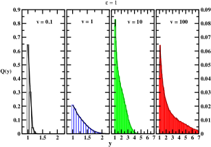
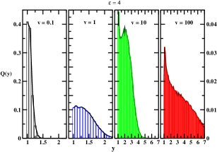
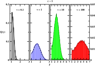
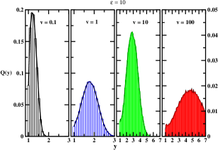
Figure 3: Distribution, $Q(y)$, of rupture tensions, $y$, for various values of the energy barrier, $\varepsilon$, and loading rate, $v$. For each row of figures, the leftmost and second leftmost figures have the same scales in both $x$ and $y$ axes, and likewise for rightmost and second rightmost figures. Note that $y$ - scales of rightmost figures are an order of magnitude smaller than for the leftmost ones.

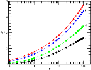
Figure 4: DTS spectrum $\langle y(\varepsilon|v)\rangle$ as a function of the loading rates $v$ (in logarithm scale) for various barrier heights $\varepsilon$ (quoted numbers). Filled symbols correspond to simulations and dashed lines are guide eyes.

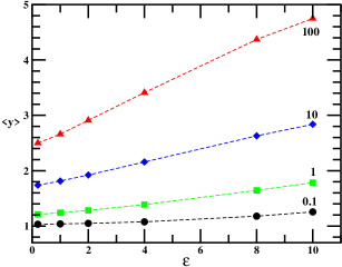
Figure 5: DTS spectrum $\langle y(\varepsilon|v)\rangle$ as a function of the barrier height $\varepsilon$ for various loading rates $v$ (quoted numbers). Filled symbols correspond to simulations and dashed lines are guide eyes.

V.2 Finite Pore Nucleation Rate $q\neq 0$ limit

To investigate the effect of pore nucleation rate on the membrane rupture, we consider two cases of increasing complexity.

V.2.1 $\alpha=0$ limit

In this case, $k_{\rm n,eff}=k_{\rm n}=q_{0}$. Figure 6 shows the variation of rupture rate $k(\varepsilon|v)$ as a function of the pore nucleation rate $q_{0}$. As expected for a successive process, $k(\varepsilon|v)$ linearly grows with $q_{0}$ in the nucleation controlled limit when $q_{0}\ll k_{d}$ and saturates to $k_{d}$ in the diffusion controlled limit for $q_{0}\gg k_{d}$. Figure 6 illustrates that system parameters can be tuned to follow the transition between the nucleation and diffusion controlled limits. Accordingly, Fig. 7 displays the profiles of the distribution $Q(y)$ corresponding to the nucleation controlled limit and toward the diffusion controlled limit.

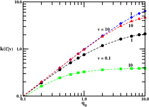
Figure 6: Rupture rate $k(\varepsilon|v)$ as a function of the tension independent pore nucleation rate $q_{0}$ (for $\alpha=0$) for various barrier heights $\varepsilon$ (quoted numbers) and loading rates $v=0.1$ (circles and squares) and $v=10$ (diamonds and triangles). Filled symbols correspond to simulations and dashed lines are guide eyes.

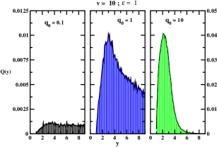
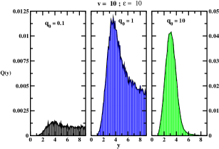
Figure 7: Distribution, $Q(y)$, of rupture tensions, $y$, for various values of the tension independent pore nucleation rate, $q_{0}$ (for $\alpha=0$), and loading rate, $v$. For each row of figures, panels with $q_{0}=1$ and $q_{0}=10$ have the same scales in both $x$ and $y$ axes.

V.2.2 Case of $\alpha=1$

When $\alpha\neq 0$, the dynamic nature of membrane rupture leads to $k_{\rm n,eff}\neq k_{\rm n}$. Both $k(\varepsilon|v)$ and $Q(y)$ still exhibit similar behaviors observed in the case of $\alpha=0$ but with nontrivial dependence on the loading rate $v$ and barrier height $\varepsilon$. As $k_{d}(\varepsilon|v)$ is known from the limit $q\rightarrow\infty$, the behavior of $k_{\rm n,eff}(\varepsilon|v)$ can be learned from Fig. 8. Clearly, $k_{\rm n,eff}\geq k_{\rm n}$, and the effective pore nucleation rate has extra $v$ and $\varepsilon$ dependencies that are not taken into account in $k_{\rm n}$ in the absence of pore dynamics. The departure of $k_{\rm n,eff}$ from $k_{\rm n}$ increases with both $v$ and $\varepsilon$ indicating that opening pore is more likely for high barrier membrane with high loading rates. The kind of distributions $Q(y)$ that can be observed in this limit are displayed in Fig. 9.

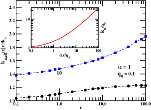
Figure 8: Reduced effective nucleation rate $k_{\rm n,eff}(\varepsilon|v)/k_{n}(v)$ as a function of the loading rates $v$ in log-linear scale for various barrier heights $\varepsilon$ (quoted numbers), with $q_{0}=0.1$ and $\alpha=1$. Filled symbols correspond to simulations and dashed lines are guide eyes. Inset: Reduced nucleation rate $k_{n}/q_{0}$ versus the variable $\alpha v/q_{0}$ in log-log scale.

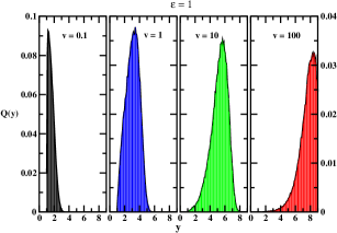
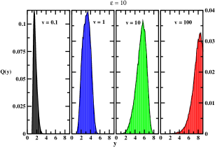
Figure 9: Distribution, $Q(y)$, of rupture tensions, $y$, for various values of loading rate, $v$, and energy barrier, $\varepsilon$, with $q_{0}=0.1$ and $\alpha=1$. For each row of figures, panels with $v=1$, $v=10$ and $v=100$ have the same scales in both $x$ and $y$ axes.

VI Concluding Remarks

Rupturing fluid membranes or vesicles with a steady ramp of micropipette suction produces a distribution of breakage tensions governed by the kinetic process. Experimental evidences have demonstrated that the membrane rupture is a dynamical property whose the strength depends on the time scale for breakage. From the theoretical point of view, we have developed a minimal model for the Dynamic Tension Spectroscopy that describes the pore nucleation as a first-order activated process, the dynamics of pore growth as a two-dimensional (in pore radius and tension spaces) Markovian stochastic process, and the rupturing of membrane is modeled by an escape process over the time-dependent critical barrier of the energy landscape. We have provided an exact analytical solution of this problem and established the correspondence between this description and the three-state model in Ref. EHLR03 . As numerical results, we have simulated the rupture rate and the distribution of rupture tension as a function of the pore nucleation rate, the critical barrier height, $\varepsilon$, of the unstressed membrane and the reduced tension loading rate, $v$. Our simulated histograms reproduce already several features observed in DTS experiments in EHLR03 and highlight the variety of profiles and richness of the problem. Indeed, the distribution of rupture tensions show different profiles between and in the two nucleation and diffusion controlled limits as a function of $\varepsilon$ and $v$.

As presented above, the kinetic of membrane rupture as probed in DTS experiments is very similar to non-equilibrium problems studied in single-molecule pulling experiments using atomic-force microscopes BQG86 ; MA88 . To cite a few, there are several theoretical works BE78 ; ER97 ; ISB97 ; HS03 ; OHS06 that have been developed, extended and refined to describe the thermally activated rupture events within the general framework of Kramers reaction rate theory Kra40 ; HTB90 .

Needless to recall that the theoretical model outlined above does not yet take into account all aspects of the membrane rupture observable in the experiments since we purposely neglected some of features like, e.g., the coarse-grained structure of the membrane. However, the developed formulation can be embellished in several directions to include the mentioned above and some other ingredients, like, non-Markovian dynamics of the pore radius dynamics driven by the membrane matrix in which the pore is embedded, and eventually, the time variation of barrier energy $\varepsilon$ due to change of the line tension. Such a generalized reaction rate approach can be also applied to membrane disruption by antimicrobial peptides. Indeed a peptide binding causes a local membrane area expansion and therefore it is equivalent to local tension (see more about the problem in HU06 ; BJ07 ). Such a work is underway.

References

- (1) S. A. Paula, A. G. Volkov, A. N. Van Hoeck, T. H. Haines, and D. W. Deamer, Biophys. J. 70, 339 (1996).
- (2) S. A. Safran,T. L. Kuhl, and J. N. Israelachvili, Biophys. J. 81, 859 (2001).
- (3) R. W. Glaser, S. L. Leikin, L. V. Chernomordik, V. F. Pastushenko, and A. I. Sokirko, Biochim. Biophys. Acta 940, 275 (1988).
- (4) D. P. Tieleman, H. Leontiadou, A. E. Mark, and S-J. Marriuk, J. Am. Chem. Soc. 125, 6382 (2003).
- (5) H. W. Huang, Biochim. Biophys. Acta 1758, 1292 (2006).
- (6) E. Evans, V. Heinrich, F. Ludwig, and W. Rawicz, Biophys. J. 85, 2342 (2003).
- (7) H. A. Kramers, Physica 7, 284 (1940).
- (8) P. Hänggi, P. Talkner, and M. Borkovec, Rev. Mod. Phys. 62, 251 (1990).
- (9) L. Fournier and B. Joos, Phys. Rev. E., 67, 051908 (2003).
- (10) P-A. Boucher, B. Joos, M. J. Zuckermann, and L. Fournier, Biophys. J., 92, 4344 (2007).
- (11) S. Safran, Statistical Thermodynamics of Surfaces, Interfaces and Membranes (Addison-Wesley, New York, 1994).
- (12) J. D. Litster, Phys. Lett. A 53, 193 (1975).
- (13) A. Szabo, K. Schulten, and Z. Schulten, J. Chem. Phys. 72, 4350 (1980).
- (14) D. J. Bicout and A. Szabo, J. Chem. Phys. 106, 10292 (1997).
- (15) R. Zwanzig, Nonequilibrium Statistical Mechanics (Oxford University Press, New York, 2001).
- (16) M. Abramowitz and I. A. Stegun Handbook of Mathematical Function (Dover, New York, 1972), p. 686.
- (17) G. Binning, C. F. Quate, and G. Gerber, Phys. Rev. Lett. 56, 930 (1986).
- (18) G. Meyer and N. M. Amer, Appl. Phys. Lett. 53, 1045 (1988).
- (19) G. I. Bell, Science 200, 618 (1978).
- (20) E. Evans and K. Ritchie, Biophys. J. 72, 1541 (1997).
- (21) S. Izrailev, S. Stepaniants, M. Balsera, Y. Oono, and K. Schulten, Biophys. J. 72, 1568 (1997).
- (22) G. Hummer and A. Szabo, Biophys. J. 85, 5 (2003).
- (23) O. K. Dudko, G. Hummer, and A. Szabo, Phys. Rev. Lett. 96, 108101 (2006).