Constraining the properties of $K_{l3}$ form factors with analyticity and unitarity

Abstract:

Bounds on the shape parameters of $K_{l3}$ form factors are investigated in a general model independent framework. Using the method of unitarity bounds for correlators evaluated in pQCD, chiral symmetry and experimental information on the phase and modulus of $\pi K$ form factors up to an energy $t_{\rm in}=1{\rm GeV}^{2}$, we constrain the shape parameters of the scalar and vector form factors, the value of the scalar form factor at $t=M_{\pi}^{2}-M_{K}^{2}$, and exclude regions where zeros can exist on the real energy line and in the complex energy plane.

1 Introduction

Strangeness changing leptonic decays of kaons are an important test of the standard model. In particular, the $K_{l3}$ decays

$$K\rightarrow\pi+l+\nu_{l},\,l=e,\,\mu$$ (1)

are a sensitive probe of QCD at low energies [1]. In addition, these decays provide for the most precise determination of the Cabibbo-Kobayashi-Maskawa (CKM) matrix element $V_{us}$ [2, 3], crucial for testing the unitarity of the CKM matrix. The dominant source of uncertainty in the extraction of $V_{us}$, resides in the experimentally determined quantity $|f_{+}(0)V_{us}|$. The $K_{\ell 3}$ decay rates were measured by BNL-E865, KLOE, KTEV, ISTRA+ and NA48, for a recent review see [4]. The decay of a kaon to a pion, charged lepton and a neutrino is described by the matrix element

$$\langle\pi^{0}(p^{\prime})|\overline{s}\gamma_{\mu}u|K^{+}(p)\rangle=\frac{1}{\sqrt{2}}[(p^{\prime}+p)_{\mu}f_{+}(t)+(p-p^{\prime})_{\mu}f_{-}(t)],$$ (2)

where $f_{+}(t)$ is the vector form factor and the combination

$$f_{0}(t)=f_{+}(t)+\frac{t}{M_{K}^{2}-M_{\pi}^{2}}f_{-}(t)$$ (3)

is known as the scalar form factor. The matrix element for the charged pion and the neutral kaon is related to Eq. (3) by isospin symmetry. For the scalar form factor, expansion at $t=0$

$$f_{0}(t)=f_{+}(0)\left(1+\lambda_{0}^{\prime}\,\frac{t}{M_{\pi}^{2}}+\frac{1}{2}\lambda_{0}^{\prime\prime}\,\frac{t^{2}}{M_{\pi}^{4}}+\cdots\right),$$ (4)

defines the slope $\lambda_{0}^{\prime}$ and the curvature $\lambda_{0}^{\prime\prime}$ parameters. Analogously we define the expansion for the vector form factor. For a precise determination of $|V_{us}|$, it is important to improve the accuracy of the parameterizations of the form factors using additional theoretical and experimental information. We use inputs from current algebra, perturbative QCD, lattice and chiral perturbation theory to provide stringent bounds on the slope and curvature parameters of the parameterizations of the form factors. More detailed discussions may be found in [5, 6, 7].

2 Formalism

Analyticity is the ideal tool for relating the information from the unitarity cut to the semileptonic range. The formalism applied in this work (see also [5, 6, 7]) exploits the fact that a bound on an integral involving the modulus squared of the form factors along the unitarity cut is known from the dispersion relation satisfied by a certain QCD correlator. For scalar form factor this reads

$$\chi_{{}_{0}}(Q^{2})\equiv\frac{\partial}{\partial q^{2}}\left[q^{2}\Pi_{0}\right]=\frac{1}{\pi}\int_{t_{+}}^{\infty}\!dt\,\frac{t{\rm Im}\Pi_{0}(t)}{(t+Q^{2})^{2}}\,,$$ (5)

$${\rm Im}\Pi_{0}(t)\geq\frac{3}{2}\frac{t_{+}t_{-}}{16\pi}\frac{[(t-t_{+})(t-t_{-})]^{1/2}}{t^{3}}|f_{0}(t)|^{2}\,,$$ (6)

with $t_{\pm}=(M_{K}\pm M_{\pi})^{2}$. Similar expression, involving the correlator $\chi_{1}(Q^{2})$, can be written down for the vector form factor. We can now use the conformal map $t\to z(t)$

$$z(t)=\frac{\sqrt{t_{+}}-\sqrt{t_{+}-t}}{\sqrt{t_{+}}+\sqrt{t_{+}-t}}\,,$$ (7)

that maps the cut $t$-plane onto the unit disc $|z|<1$ in the $z\equiv z(t)$ plane, with $t_{+}$ mapped onto $z=1$, the point at infinity to $z=-1$ and the origin to $z=0$. This mapping transforms the relations Eqs. (5) and (6) to

$${1\over 2\pi}\int_{0}^{2\pi}d\theta|g(\exp(i\theta))|^{2}\leq I$$ (8)

where

$$g(z)=f_{0}(t(z))w(z).$$ (9)

The function $w(z)$ is called outer function and can be calculated analytically in our case. The function $g(z)$ is analytic within the unit disc and can be expanded as:

$$g(z)=g_{0}+g_{1}z+g_{2}z^{2}+\cdots,$$ (10)

and Eq. (8) implies

$$\sum_{k=0}^{\infty}g_{k}^{2}\leq I.$$ (11)

Truncating the above series after finite number of terms gives equations for constraints on the shape parameters. Improvement of the bound results if $f_{0}(t)$ is known at a number of real points $t_{i}$. Using a Lagrange multiplier method, we get a determinantal inequality which leads to a quadratic form in the shape parameters that is bounded by a known quantity. In order to exploit the knowledge of the phase, the dispersion contribution from $t_{+}$ to $t_{\rm in}$ should be subtracted from the pQCD value,

$$I^{\prime}=\chi_{0}(Q^{2})-\frac{3}{2}\frac{t_{+}t_{-}}{16\pi^{2}}\int_{t_{+}}^{t_{\rm in}}\!dt\,\frac{[(t-t_{+})(t-t_{-})]^{1/2}|f_{0}(t)|^{2}}{t^{2}(t+Q^{2})^{2}}\,,$$ (12)

which requires the knowledge of $|f_{0}{(t)}|^{2}$ in the region $t_{+}\leq t\leq t_{\rm in}$. Now Eqs. (5) and (6) can be written in the following form

$$\int_{t_{\rm in}}^{\infty}{\rm d}t\rho(t)|{\cal{O}}(t)|^{2}|h(t)|^{2}\leq I^{\prime}$$ (13)

for a known weight function $\rho(t)$, and where the function $h(t)$ is analytic in the $t$-plane cut for $t>t_{\rm in}$ and given by

$$h(t)=f_{0}(t)[{\cal{O}}(t)]^{-1},$$ (14)

where we implement the phase information by considering the Omnès function:

$${\cal{O}}(t)=\exp\left(\displaystyle\frac{t}{\pi}\int^{\infty}_{t_{+}}dt\displaystyle\frac{\delta(t^{\prime})}{t^{\prime}(t^{\prime}-t)}\right),$$ (15)

where $\delta(t)$ is the $I=1/2$ elastic S-wave $K\pi$ scattering phase, in the elastic region and arbitrarily Lipschitz continuous above $t_{\rm in}$, leading to an extended formalism. This is based on the observation first made in [8] which points out that the phase of the Omnès function can compensate for that of the form factor in the region ($t_{+},$ $t_{\rm in}$), thereby delaying the onset of the branch point to $t_{\rm in}$. The Eq. (13) can be brought into a canonical form by making the conformal transformation

$$\tilde{z}(t)=\frac{\sqrt{t_{\rm in}}-\sqrt{t_{\rm in}-t}}{\sqrt{t_{\rm in}}+\sqrt{t_{\rm in}-t}}\,,$$ (16)

which maps the complex $t$-plane cut for $t>t_{\rm in}$ onto the unit disk in the $z$-plane defined by $z=\tilde{z}(t)$. Now Eq. (13) can be written as

$$\frac{1}{2\pi}\int^{2\pi}_{0}{\rm d}\theta|g(\exp(i\theta))|^{2}\leq I^{\prime}.$$ (17)

The function $g(z)$ is now defined by

$$g(z)=w(z)\,\omega(z)\,f_{0}(\tilde{t}(z))\,[O(z)]^{-1},$$ (18)

where the outer function for the Omnès function given by:

$$\omega(z)=\exp\left(\displaystyle\frac{\sqrt{t_{\rm in}-\tilde{t}(z)}}{\pi}\int^{\infty}_{t_{\rm in}}{\rm d}t^{\prime}\displaystyle\frac{\ln|{\cal{O}}(t^{\prime})|}{\sqrt{t^{\prime}-t_{\rm in}}(t^{\prime}-\tilde{t}(z))}\right).$$ (19)

For more information and the review of the formalism, see [5, 6, 7].

3 Experimental and theoretical information

We briefly give a description of different inputs used for deriving the improved bounds.

3.1 QCD correlators

In the limit $Q^{2}>>\Lambda^{2}_{QCD}$, the correlators $\chi_{1}(Q^{2})$ and $\chi_{0}(Q^{2})$ can be calculated by perturbative QCD. Recent calculations to order $\alpha_{s}^{4}$ [9, 10] give

$$I_{+}=\chi_{1}(Q^{2})=\frac{1}{8\pi^{2}Q^{2}}(1+\frac{\alpha_{s}}{\pi}-0.062\alpha_{s}^{2}-0.162\alpha_{s}^{3}-0.176\alpha_{s}^{4}),$$ (20)

$$I_{0}=\chi_{0}(Q^{2})=\frac{3(m_{s}-m_{u})^{2}}{8\pi^{2}Q^{2}}(1+1.80\alpha_{s}+4.65\alpha_{s}^{2}+15.0\alpha_{s}^{3}+57.4\alpha_{s}^{4}).$$ (21)

We have omitted the power corrections due to nonzero masses and QCD condensates, as they are negligible. We get $\chi_{1}(2\,\text{GeV})=(343.8\pm 51.6)\times 10^{-5}\,{\rm GeV}^{-2}$ and $\chi_{0}(2\,\text{GeV})=(253\pm 68)\times 10^{-6}$.

3.2 Low-energy theorems

The symmetries of QCD at low energies are very useful sources of information for our formalism. The vector form factor becomes equal to the scalar form factor at $t=0$. The SU(3) symmetry implies $f_{+}(0)=1$. The deviations from this limit are small due to Ademollo-Gatto theorem. Recent determinations from the lattice give $f_{+}(0)=0.964(5)$ [11]. In the case of the scalar form factor, current algebra relates the value of the scalar form factor at the Callan-Treiman (CT) point $\Delta_{K\pi}\equiv M_{K}^{2}-M_{\pi}^{2}$ to the ratio $F_{K}/F_{\pi}$ of the decay constants [12, 13]:

$$f_{0}(\Delta_{K\pi})=F_{K}/F_{\pi}+\Delta_{CT}.$$ (22)

In isospin limit, $\Delta_{CT}=-3.1\times 10^{-3}$ to one loop [14] and $\Delta_{CT}\simeq 0$ to two-loops in chiral perturbation theory [15, 16, 17]. At $\bar{\Delta}_{K\pi}(=-\Delta_{K\pi})$, a soft-kaon result [18] relates the value of the scalar form factor to $F_{\pi}/F_{K}$

$$f_{0}(-\Delta_{K\pi})=F_{\pi}/F_{K}+\bar{\Delta}_{CT}.$$ (23)

Recent lattice evaluations give $F_{K}/F_{\pi}=1.193\pm 0.006$ [19, 20]. A calculation in ChPT to one-loop in the isospin limit [14] gives $\bar{\Delta}_{CT}=0.03$, but the higher order ChPT corrections are expected to be larger in this case. In the present work we use as input the values of the vector and scalar form factor at $t=0$. For the scalar form factor we impose also the value $f_{0}(\Delta_{K\pi})$ at the first CT point. As discussed in [7], due to the poor knowledge of $\bar{\Delta}_{CT}$, the low-energy theorem Eq.(23) is not useful for further constraining the shape of the $K_{\ell 3}$ form factors at low energies. On the other hand we obtain bounds on $\bar{\Delta}_{CT}$.

3.3 Phase and modulus along the elastic region of the cut

As mentioned in Sec. 2 the bounds can be improved if the phase of the form factor along the elastic part of the unitarity cut is known from an independent source. According to the Fermi-Watson theorem, the phase of the form factor coincides with the phase of the scattering amplitude along the elastic part of the unitarity cut. In our calculations we use below $t_{\rm in}$ the phases from [21, 22] for the scalar form factor, and from [23, 24] for the vector form factor. We recall that, while the standard dispersion approaches require a choice of the phase above the inelastic threshold $t_{\rm in}$, the present formalism is independent of this ambiguity [6]. Above $t_{\rm in}$ we have taken $\delta(t)$ as a smooth function approaching $\pi$ at high energies. The results are independent of the choice of the phase for $t>t_{\rm in}$. We have checked numerically this independence with high precision.

To estimate the low-energy integral in Eq. (12), we use the Breit-Wigner parameterizations of $|f_{+}(t)|$ and $|f_{0}(t)|$ in terms of the resonances given by the Belle Collaboration [25] for fitting the rate of $\tau\to K\pi\nu$ decay. This leads to the value $31.4\times 10^{-5}\,{\rm GeV}^{-2}$ for the vector form factor and $60.9\times 10^{-6}$ for the scalar form factor. By combining with the values of $I_{+,0}$ defined in Eqs. (20)-(21), we obtain

$$I_{+}^{\prime}=(312\pm 69)\times 10^{-5}\,{\rm GeV}^{-2},\quad I_{0}^{\prime}=(192\pm 90)\times 10^{-6}.$$ (24)

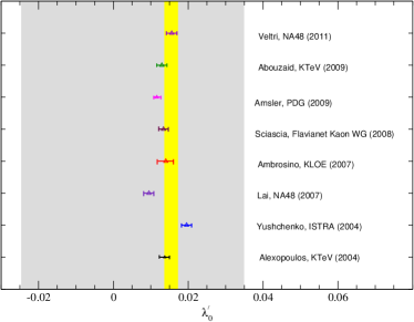
Figure 1: The allowed range for the slope of the scalar form factor, when we include phase, modulus and the Callan-Treiman constraint (yellow band). The grey band shows the range without using the Callan-Treiman constraint.

4 Results

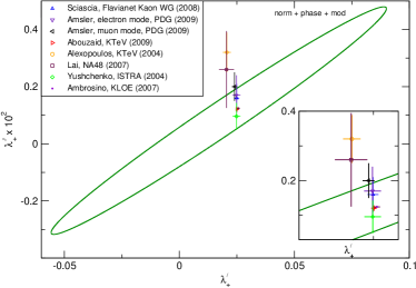
Figure 2: The best constraints for the slope and curvature of the vector form factor in the slope-curvature plane, where the allowed region is the interior of the ellipse.

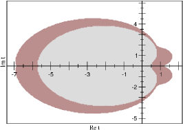
Figure 3: Domain without zeros for the scalar form factor: the small domain is obtained without including phase and modulus in the elastic region, bigger one using phase, modulus and Callan-Treiman constraint.

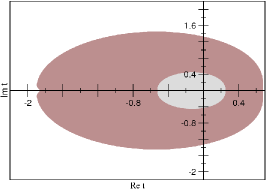
Figure 4: Domain without zeros for the vector form factor: the small domain is obtained without including phase and modulus in the elastic region, bigger one using phase and modulus.

In Fig. 1, the allowed band for the slope $\lambda_{0}^{\prime}$ is compared with the experimental determinations. The slope predicted by NA48 (2007) is not consistent with our predictions. However their recent determination confirms our predicted range, see Veltri et.al [4]. We note that the theoretical prediction of ChPT to two loops $\lambda_{0}^{\prime}=(13.9_{+1.3}^{-0.4}\pm 0.4)\times 10^{-3}$, $\lambda_{0}^{\prime\prime}=(8.0_{+0.3}^{-1.7})\times 10^{-4}$ is consistent within errors. For the central value of the slope $\lambda_{0}^{\prime}$ given above, the range of $\lambda_{0}^{\prime\prime}$ is $(8.24\times 10^{-4},8.42\times 10^{-4})$. The same is true for the theoretical prediction $\lambda_{0}^{\prime}=(16.00\pm 1.00)\times 10^{-3}$, $\lambda_{0}^{\prime\prime}=(6.34\pm 0.38)\times 10^{-4}$ obtained from dispersion relations.

As shown in Fig. 2 for vector form factor, except the results from NA48 and KLOE, which have curvatures slightly larger than the allowed values, the experimental data satisfy the constraints. We note also that the theoretical predictions $\lambda_{+}^{\prime}=(24.9\pm 1.3)\times 10^{-3}$, $\lambda_{+}^{\prime\prime}=(1.6\pm 0.5)\times 10^{-3}$ obtained from ChPT to two loops, and $\lambda_{+}^{\prime}=(26.05_{-0.51}^{+0.21})\times 10^{-3}$, $\lambda_{+}^{\prime\prime}=(1.29_{-0.04}^{+0.01})\times 10^{-3}$, and $\lambda_{+}^{\prime}=(25.49\pm 0.31)\times 10^{-3}$, $\lambda_{+}^{\prime\prime}=(1.22\pm 0.14)\times 10^{-3}$ obtained from dispersion relations are consistent with the constraint. For precise results, see [5]. As we mentioned, the same formalism can be used to derive regions in the complex plane where the form factors can not vanish. In Fig. 4 we show the region where zeros of the scalar form factors are excluded. If we impose the Callan-Treiman constraint, the value of $f_{0}(\Delta_{K\pi})$, the scalar form factor cannot have simple zeros in the range $-1.81\,\mbox{GeV}^{2}\leq t_{0}\leq 0.93\,\mbox{GeV}^{2}$. The formalism rules out zeros in the physical region of the kaon semileptonic decay. In the case of complex zeros, we have obtained a rather large region where they cannot be present.

For the vector form factors, simple zeros are excluded in the interval $-0.31\,\mbox{GeV}^{2}\leq t_{0}\leq 0.23\,\mbox{GeV}^{2}$ of the real axis, while Fig. 4 shows the region where complex zeros are excluded. For more results, see [5]. We mention that we do not use as input the soft-kaon theorem, but derive bounds on the value at the relevant point. Thus we are able to predict a narrow range $-0.046\leq\bar{\Delta}_{CT}\leq 0.014$ for higher order corrections.

5 Conclusion

We have studied the shape of the scalar and vector form factors in the $K_{\ell 3}$ domain, crucial for the determination of the modulus of the CKM matrix element $|V_{us}|$. The results are very stringent in the scalar form factor case. The most recent results from NA48 [4] is consistent with our prediction for the slope of scalar form factor and restricts the range of the slope to $\sim 0.01-0.02$.

Our results show that the zeros are excluded in a rather large domain at low energies, which provides confidence in semiphenomenological analyses based on Omnès representations which assume that the zeros are absent. Unlike the standard dispersive treatments, our method does not require the knowledge of zeros and of the phase above the inelastic threshold. Therefore, model dependent assumptions are not necessary. The price to pay is that we only are able to predict ranges for shape parameters and zero positions. However, due to the high precision of low energy measurements and calculations, the predicted bounds are very stringent.

References

- [1] L. -M. Chounet, J. -M. Gaillard and M. K. Gillard, Phys. Rept. 4 (1972) 199.
- [2] M. Antonelli, V. Cirigliano, G. Isidori, F. Mescia, M. Moulson, H. Neufeld, E. Passemar and M. Palutan et al., Eur. Phys. J. C 69 (2010) 399 [arXiv:1005.2323 [hep-ph]].
- [3] V. Cirigliano, G. Ecker, H. Neufeld, A. Pich and J. Portoles, arXiv:1107.6001 [hep-ph].
- [4] M. Veltri, arXiv:1101.5031 [hep-ex].
- [5] G. Abbas, B. Ananthanarayan, I. Caprini and I. Sentitemsu Imsong, Phys. Rev. D 82 (2010) 094018 [arXiv:1008.0925 [hep-ph]].
- [6] G. Abbas, B. Ananthanarayan, I. Caprini, I. Sentitemsu Imsong and S. Ramanan, Eur. Phys. J. A 45 (2010) 389 [arXiv:1004.4257 [hep-ph]].
- [7] G. Abbas, B. Ananthanarayan, I. Caprini, I. Sentitemsu Imsong and S. Ramanan, Eur. Phys. J. A 44 (2010) 175 [arXiv:0912.2831 [hep-ph]].
- [8] I. Caprini, Eur. Phys. J. C 13 (2000) 471 [hep-ph/9907227].
- [9] P. A. Baikov, K. G. Chetyrkin and J. H. Kuhn, Phys. Rev. Lett. 96 (2006) 012003 [hep-ph/0511063].
- [10] P. A. Baikov, K. G. Chetyrkin and J. H. Kuhn, Phys. Rev. Lett. 101 (2008) 012002 [arXiv:0801.1821 [hep-ph]].
- [11] P. A. Boyle, A. Juttner, R. D. Kenway, C. T. Sachrajda, S. Sasaki, A. Soni, R. J. Tweedie and J. M. Zanotti, Phys. Rev. Lett. 100 (2008) 141601 [arXiv:0710.5136 [hep-lat]].
- [12] C. G. Callan and S. B. Treiman, Phys. Rev. Lett. 16 (1966) 153.
- [13] R. F. Dashen and M. Weinstein, Phys. Rev. Lett. 22 (1969) 1337.
- [14] J. Gasser and H. Leutwyler, Nucl. Phys. B 250 (1985) 517.
- [15] A. Kastner and H. Neufeld, Eur. Phys. J. C 57 (2008) 541 [arXiv:0805.2222 [hep-ph]].
- [16] J. Bijnens and P. Talavera, Nucl. Phys. B 669 (2003) 341 [hep-ph/0303103].
- [17] J. Bijnens and K. Ghorbani, arXiv:0711.0148 [hep-ph].
- [18] R. Oehme, Phys. Rev. Lett. 16, (1966) 215 .
- [19] L. Lellouch, PoS LATTICE 2008 (2009) 015 [arXiv:0902.4545 [hep-lat]].
- [20] S. Durr, Z. Fodor, C. Hoelbling, S. D. Katz, S. Krieg, T. Kurth, L. Lellouch and T. Lippert et al., Phys. Rev. D 81 (2010) 054507 [arXiv:1001.4692 [hep-lat]].
- [21] P. Buettiker, S. Descotes-Genon and B. Moussallam, Eur. Phys. J. C 33 (2004) 409 [hep-ph/0310283].
- [22] B. El-Bennich, A. Furman, R. Kaminski, L. Lesniak, B. Loiseau and B. Moussallam, Phys. Rev. D 79 (2009) 094005 [Erratum-ibid. D 83 (2011) 039903] [arXiv:0902.3645 [hep-ph]].
- [23] B. Moussallam, Eur. Phys. J. C 53 (2008) 401 [arXiv:0710.0548 [hep-ph]].
- [24] V. Bernard, M. Oertel, E. Passemar and J. Stern, Phys. Rev. D 80 (2009) 034034 [arXiv:0903.1654 [hep-ph]].
- [25] D. Epifanov et al. [Belle Collaboration], Phys. Lett. B 654 (2007) 65 [arXiv:0706.2231 [hep-ex]].