Spectral properties of thermal fluctuations on simple liquid surfaces below shot noise levels

Abstract

We study the spectral properties of thermal fluctuations on simple liquid surfaces, sometimes called ripplons. Analytical properties of the spectral function are investigated and are shown to be composed of regions with simple analytic behavior with respect to the frequency or the wave number. The derived expressions are compared to spectral measurements performed orders of magnitude below shot noise levels, which is achieved using a novel noise reduction method. The agreement between the theory of thermal surface fluctuations and the experiment is found to be excellent.

I Introduction

Thermal fluctuations are ubiquitous and exist for practically everything we see and touch. However, they tend to be too small to be observed or measured directly, except under special circumstances. Phenomena in which thermal fluctuations can be examined directly in non-exotic materials are surface fluctuations of liquids, sometimes called “ripplons”ripplon . Using surface light scattering, thermal surface fluctuations of liquids have been studied for some timeripplonExp . Other direct thermal fluctuation measurements include high power interferometry of mirror surfacesmirror and fluctuations of surfaces with exceptionally low surface tensiongiant .

In this work, we detect reflected light from surfaces to measure their inclinationsopticalLever ; Tay ; am1 and apply this to thermal surface fluctuations of simple liquids. The measurements are somewhat complementary to the spectral measurements performed at specific wavelengths. The measurements require less power, can be performed on smaller samples and can be applied to strongly viscous fluids. Furthermore, the measurement system can be simpler. While shot noise is often regarded as an unavoidable limitation in such measurements, we show that such is not the case. The measurements involve novel methods that allow us to measure the spectrum directly, down to several orders of magnitude below the shot noise level. As we explain, this principle is not limited to thermal noise measurements nor to surface light scattering measurements. The experimental results agree with the theory quite well. In the process, we elucidate the simple analytic behavior of the spectra and show how it is reflected in the full spectrum, which can be seen in experiments.

The dispersion relation for surface waves on a simple liquid surface can derived from the Navier-Stokes equation, when the viscosity of the liquid can be ignored, as

$$\omega(k)=\sqrt{{\sigma k^{3}\over\rho}+gk}\qquad.$$ (1)

Here, $g$ is the gravitational acceleration, $\rho,\sigma$ are the density and the surface tension of the liquid, $k$ is the wave number and $\omega$ is the (angular) frequency. The viscosity becomes more important for shorter wavelengths and dissipation will play an essential role below. Gravitational effects are more important for longer wavelengths and is negligible for wavelengths much smaller than $\pi\sqrt{\sigma/(\rho g)}$. For liquids we examine, namely, water, ethanol and oil, gravitational effects are unimportant for scales below $10\,$mm. The samples we examine have surface sizes of few mm and longer wavelengths are effectively cut off, so that henceforth we ignore effects due to gravity. Under these circumstances, the dispersion relation reduces to the following two equivalent relationships.

$$\omega=\omega_{R}(k)=\sqrt{\sigma k^{3}\over\rho}\qquad,\qquad k=k_{R}(\omega)=\left(\rho\omega^{2}\over\sigma\right)^{1/3}\qquad.$$ (2)

In what follows, we examine the full spectrum both experimentally and theoretically, including the full effects of dissipation.

The paper is organized as follows: In Sect. II, we explain the surface light reflection experiment and derive what precisely is measured by this. The properties of thermal surface fluctuations of simple liquids are examined in Sect. III and the approximate simple analytic behavior of the spectra are derived. The shot noise level in our experiments are assessed in Sect. IV. The noise reduction method explained in Sect. V allows us to detect weak signals buried under the shot noise level. The general applicability of the principle is also clarified. Finally, we combine the theoretical and the experimental results in Sect. VI and find that they agree. The limitations in the experiment and further directions for research are also discussed.

II The experiment and the measurement

In the experiment (Fig. 1), inclination fluctuations of a liquid surface are measured using two sets of measurement systems each with a laser beam 1 (wavelength 638 nm) and 2 (658 nm). The average inclination within the beam area essentially acts as an optical lever and the inclination deflects the laser beams to be detected by the dual-element photodiodes (DEPD 1,2, S4204 Hamamatsu Photonics, Japan)opticalLever . The two sets of photodiodes are necessary here to eliminate the random noise statistically, as explained in Sect. V. The DEPD signals are amplified and then fed into a computer via analog to digital converters (ADC, 14 bit, ADXII14-80M, Saya, Japan). Fourier transforms and averagings are performed by the computer.

The laser beam power at the sample is 0.5 mW each. The beam is focused down to $\mu$m order and its diameter ($\sim\lambda/N\!A$) is varied by changing the numerical aperture ($N\!A$) of the objective lens, where $\lambda$ is the wavelength of the probe laser beam. This beam size is considerably smaller than that used in the standard light scattering methods. The amplitude of the waves are small compared to the wavelength so that the reflected light is almost all collected by the objective lens. Therefore, compared to the standard light scattering experiments which observes only a small fraction of the scattered light, we obtain larger signals for a given beam power. This can be crucial in low power measurements.

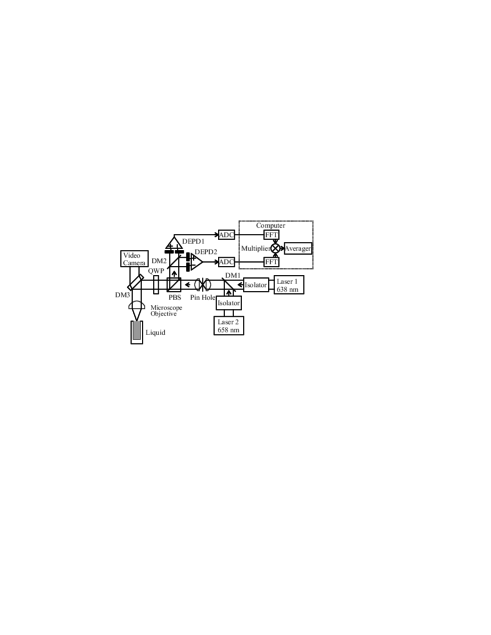
Figure 1: Two laser beams with wavelengths 638 nm and 658 nm are combined at a dichroic mirror (DM1) and focused by a microscope objective lens onto the liquid surface. The reflected light with different wavelengths are separated at DM2 to obtain two independent inclination measurements of the same surface. The inclination is converted into electric signals using DEPD1, DEPD2 and are fed via ADC’s into a computer where FFT (fast Fourier transform) and averagings are performed. A polarizing beam splitter (PBS) and a quarter wave plate (QWP) are included to extract the light reflected back from the sample efficiently. DM3 is used for viewing the sample through a video camera.

We now explain what is measured in this experiment and how this relates to the spectrum of surface fluctuations. We measure fluctuations in the average inclination of the surface. Denoting the surface level as $\phi(\bm{r},t)$, the average inclination $a_{1}(t)$ can be obtained by approximating $\phi(\bm{r},t)$ by a linear profile, minimizing the following quantity:

$$\int d^{2}\bm{r}\,G(\bm{r})\left|\phi(\bm{r},t)-\left(a_{0}(t)+a_{1}(t)x\right)\right|^{2}\qquad.$$ (3)

Here, $\bm{r}=(x,y)$ are coordinates on the surface and $G(\bm{r})$ is the beam intensity profile. This leads to the expression for the average displacement and inclination,

$$a_{0}(t) = C_{0}\int d^{2}\bm{r}\,G(\bm{r})\phi(\bm{r},t)\quad,\quad C_{0}=\left(\int d^{2}\bm{r}\,G(\bm{r})\right)^{-1}\qquad,$$ (4)

$$a_{1}(t) = C_{1}\int d^{2}\bm{r}\,G(\bm{r})x\phi(\bm{r},t)\quad,\quad C_{1}=\left(\int d^{2}\bm{r}\,x^{2}G(\bm{r})\right)^{-1}\qquad.$$ (5)

While we can solve for $a_{j}(t)$ more generally, we assumed here that the profile is symmetric, $\int d^{2}\bm{r}\,xG(\bm{r})=0$, which applies to our case, as discussed below. We define the Fourier transform of $a_{j}$ as

$$\tilde{a}_{j}(\omega)={1\over\sqrt{T}}\int^{T/2}_{-T/2}\!\!dt\,e^{i\omega t}a_{j}(t)\quad,\qquad j=1,2\qquad,$$ (6)

where $T$ is the measurement time, which is much longer when compared to the other time scales involved.

Since the correlation function of the surface fluctuations is translation invariant both in space and time, it can be expressed as

$$\langle\phi(\bm{r},t)\phi(\bm{r}^{\prime},t^{\prime})\rangle=\int{d\omega\over 2\pi}\int{d^{2}\bm{k}\over(2\pi)^{2}}\,e^{i\bm{k}(\bm{r}-\bm{r}^{\prime})-i\omega(t-t^{\prime})}P(k,\omega)\qquad.$$ (7)

Here, $P(k,\omega)$ is the spectral function of the fluctuations of the surface displacement and $\langle\cdots\rangle$ denotes the statistical average. Using this correlation function, the fluctuations in the inclinations are obtained as

$$\langle|\tilde{a}_{1}(\omega)|^{2}\rangle=\int{d^{2}\bm{k}\over(2\pi)^{2}}\,\left|C_{1}\int d^{2}\bm{r}\,e^{i\bm{k}\bm{r}}xG(\bm{r})\right|^{2}P(k,\omega)\qquad.$$ (8)

Since we are using a laser beam well described by a Gaussian profile to observe surface fluctuations, the profile function $G(\bm{r})$ can be expressed using the beam diameter $b$ as

$$G(\bm{r})=I_{0}e^{-8r^{2}/b^{2}}\qquad,$$ (9)

The spectrum measured in the experiment is (we henceforth use the notation $\omega=2\pi f$)

$$S(f)=4\pi\langle|\tilde{a}_{1}(\omega)|^{2}\rangle\qquad,$$ (10)

taking into account that the measurement is in frequency space and the one-sidedness of the spectrum. Combining the results above, we derive a compact expression for the fluctuation spectrum observed in the experiment,

$$S(f)=\int_{0}^{\infty}dk\,k^{3}e^{-b^{2}k^{2}/16}P(k,2\pi f)\qquad.$$ (11)

It should be noted that this formula applies to general surface fluctuation spectra measured using this method and is not limited to liquids nor to thermal fluctuations. This result specifies the measured spectrum $S(f)$ completely including its magnitude, given the spectral function $P(k,\omega)$ and the beam diameter $b$, and is independent of the beam power applied. As can be seen from the expression, the role of the beam size is to effectively cut off the $k$ integral of the spectral functions for values over $\sim 2\pi/b$. This occurs because the inclination is effectively averaged within the beam spot, so that shorter wavelengths are effectively averaged out. It also explains why we integrate up to infinity in this formula; while, in principle, the wavelengths of surface fluctuations should be cutoff at atomic length scales, this is much smaller than $b$ so that using infinity as the upper limit in the integration region introduces negligible difference, due to the Gaussian damping. The lower limit of the integration region should, strictly speaking, be set to $\sim 2\pi/L$, where $L$ is the size of the sample ($L$ is few mm in our experiment) providing an upper bound for wavelengths. However, the difference from setting the lower end of the integral to zero as in the formula can also be ignored, as will become clear below.

III Analytic structure of the spectrum

The spectral function for thermal fluctuations of simple liquid surfaces has been derived previouslyBouchiat ,

$$P(k,\omega)={k_{\scriptscriptstyle B}T\over\pi}{ku^{2}\over\rho\omega^{3}}{\rm\,Im}\left[(1-iu)^{2}+y-\sqrt{1-2iu}\right]^{-1},\qquad u\equiv{\rho\omega\over 2\eta k^{2}}\quad y\equiv{\rho\sigma\over 4\eta^{2}k}\qquad.$$ (12)

While this expression for the spectrum is analytic, its behavior is not apparent. The behavior can be split into several regimes depending on the viscosity. We summarize the behavior concisely below to gain insight into the behavior of the spectral function and for later use.

III.1 Leading analytic behavior with respect to $k$

Let us study the behavior of the spectral function $P(k,\omega)$ with respect to $k$ with $\omega$ fixed. The dimensionless measure of viscosity of the liquid, $\eta^{3}\omega/(\rho\sigma)$ influences the behavior of the spectral function $P(k,\omega)$ qualitatively. Any liquid is highly dissipative for high enough frequencies, which is intuitively natural. When the viscosity is effectively low, $\eta^{3}\omega/(\rho\sigma)<1/(8\sqrt{2})$, the leading order analytic behavior $P_{0}(k,\omega)$ can be obtained as

$$P_{0}(k,\omega)={k_{\scriptscriptstyle B}T\over\pi}\times\left\{\begin{array}[c]{lll}\displaystyle{{4\eta k^{3}\over\rho^{2}\omega^{4}}}&\qquad\hbox{when }&k<2^{-1/6}k_{R}(\omega)\\ &&\\ \displaystyle{{2\eta\over\sigma^{2}k^{3}}}&&k>2^{-1/6}k_{R}(\omega)\\ \end{array}\right.\qquad.$$ (13)

In this case, $P(k,\omega)$ has a peak close to $k=k_{R}(\omega)$, which becomes less prominent as $\eta^{3}\omega/(\rho\sigma)$ increases. When $\eta^{3}\omega/(\rho\sigma^{2})>1/(8\sqrt{2})$, the leading behavior of the dispersion relation splits into three regions as

$$P_{0}(k,\omega)={k_{\scriptscriptstyle B}T\over\pi}\times\left\{\begin{array}[c]{lll}\displaystyle{{4\eta k^{3}\over\rho^{2}\omega^{4}}}&\qquad\hbox{when }&\displaystyle{k<2^{-1/4}\sqrt{\rho\omega\over 2\eta}}\\ &&\\ \displaystyle{{1\over 2\eta k\omega^{2}}}&&\displaystyle{2^{-1/4}\sqrt{\rho\omega\over 2\eta}<k<{2\eta\omega\over\sigma}}\\ &&\\ \displaystyle{{2\eta\over\sigma^{2}k^{3}}}&&\displaystyle{k>{2\eta\omega\over\sigma}}\\ \end{array}\right.\qquad.$$ (14)

In both cases with low and high viscosity, for long wavelengths compared to $2\pi/k_{R}(\omega)$, the spectral function is governed by viscous behavior and depends on $\rho$. On the other hand, for short wavelengths, it is suppressed by the surface tension of the liquid and is independent of its density.

In Fig. 2, we compare the full spectral function Eq. (12) with its approximate analytic behavior derived above. We see that in all the cases, the spectrum is well reproduced by the simple analytic behaviors, except for the peak seen in the water surface fluctuations at lower frequencies. The peak behavior reflects long lived waves and disappears when the viscosity is effectively high, due to dissipation. In both Eqs. (13), (14), the spectral function is independent of $f$ for large $k$, which can be seen from the plots. The simple analytic formulas derived above capture the situations with weak and strong viscosity, which have qualitatively different behaviors.

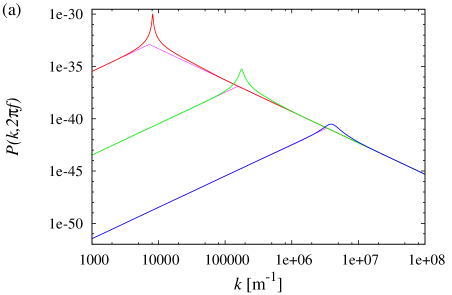
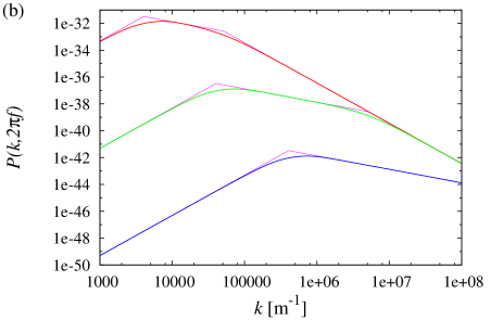
Figure 2: (Color online) Behavior of $P(k,2\pi f)$ for (a) water and (b) oil with respect to $k$ at fixed $f$. Frequencies are $f=10^{3},10^{5},10^{7}$ [s^-1] (red, green, blue lines respectively), with the maximum of the spectrum being larger for higher $f$. The corresponding simple analytic behaviors Eqs. (13),(14) are also shown (thin lines, magenta) and matches well with the full spectral function and are almost invisible, except at the boundaries between the regions.

III.2 Leading analytic behavior with respect to $\omega$

We now analyze the behavior of $P(k,\omega)$ with respect to $\omega$ for fixed $k$. For a liquid with low viscosity effectively, $\eta^{2}k/(\rho\sigma)<1/(4\sqrt{2})$, the leading order analytic behavior $P_{0}(k,\omega)$ is broken up into two regions as

$$P_{0}(k,\omega)={k_{\scriptscriptstyle B}T\over\pi}\times\left\{\begin{array}[c]{lll}\displaystyle{{2\eta\over\sigma^{2}k^{3}}}&\qquad\hbox{when }&\omega<2^{1/4}\omega_{R}(k)\\ &&\\ \displaystyle{{4\eta k^{3}\over\rho^{2}\omega^{4}}}&&\omega>2^{1/4}\omega_{R}(k)\\ \end{array}\right.\qquad.$$ (15)

For the highly viscous case, the leading analytic behavior can be broken down into three regions thus.

$$P_{0}(k,\omega)={k_{\scriptscriptstyle B}T\over\pi}\times\left\{\begin{array}[c]{lll}\displaystyle{{2\eta\over\sigma^{2}k^{3}}}&\qquad\hbox{when }&\displaystyle{\omega<{\sigma k\over 2\eta}}\\ &&\\ \displaystyle{{1\over 2\eta k\omega^{2}}}&&\displaystyle{{\sigma k\over 2\eta}<\omega<{2\sqrt{2}\eta k^{2}\over\rho}}\\ &&\\ \displaystyle{{4\eta k^{3}\over\rho^{2}\omega^{4}}}&&\displaystyle{\omega>{2\sqrt{2}\eta k^{2}\over\rho}}\\ \end{array}\right.\qquad.$$ (16)

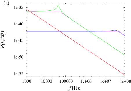
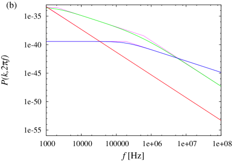
Figure 3: (Color online) Behavior of $P(k,2\pi f)$ for (a) water and (b) oil with respect to frequency $f$ at $k=10^{3},10^{5},10^{7}$ [m^-1] (red, green, blue lines respectively). The spectra with larger $k$ have more fluctuations at higher $f$. Their analytic approximations Eqs. (15), (16) (thin lines, magenta) agree well with the full spectral function and are almost invisible, except at the boundaries between the regions.

III.3 Analytic behavior of the integrated spectrum

While the spectrum $S(f)$ in Eq. (11) can be computed numerically, we now clarify its rough analytic behavior using $P_{0}(k,2\pi f)$ derived above. In the integrated spectrum $S(f)$, $b$ provides a cutoff ${k_{\rm max}}$ for the integral, whose relation we specify below. The spectrum can be approximated by

$$S_{0}(f)=\int_{0}^{{k_{\rm max}}}dk\,k^{3}P_{0}(k,2\pi f)\qquad.$$ (17)

This can be computed explicitly. For the low viscosity case $\eta^{3}\omega/(\rho\sigma^{2})<1/(8\sqrt{2})$,

$$S_{0}(f)={k_{\scriptscriptstyle B}T\over\pi}\times\left\{\begin{array}[c]{lll}\displaystyle{\left({2\eta{k_{\rm max}}\over\sigma^{2}}-{2^{11/6}3\rho^{1/3}\eta\over 7\sigma^{7/3}}\omega^{2/3}\right)}&\quad\hbox{when }&\displaystyle{\omega<2^{1/4}\omega_{R}({k_{\rm max}})}\\ &&\\ \displaystyle{{4\eta{k_{\rm max}}^{7}\over 7\rho^{2}}{1\over\omega^{4}}}&&\displaystyle{\omega>2^{1/4}\omega_{R}({k_{\rm max}})}\\ \end{array}\right.\qquad.$$ (18)

When the viscosity is high, the spectrum has the following approximate.

$$S_{0}(f)={k_{\scriptscriptstyle B}T\over\pi}\times\left\{\begin{array}[c]{lll}\displaystyle{\left({2\eta{k_{\rm max}}\over\sigma^{2}}-{8\eta^{2}\over 3\sigma^{3}}\omega-{\rho^{3/2}\over 2^{5/4}21\eta^{5/2}}{1\over\omega^{1/2}}\right)}&\quad\hbox{when }&\displaystyle{\omega<{\sigma{k_{\rm max}}\over 2\eta}}\\ &&\\ \displaystyle{\left({{k_{\rm max}}^{3}\over 6\eta}{1\over\omega^{2}}-{\rho^{3/2}\over 2^{5/4}21\eta^{5/2}}{1\over\omega^{1/2}}\right)}&&\displaystyle{{\sigma{k_{\rm max}}\over 2\eta}<\omega<{2\sqrt{2}\eta{k_{\rm max}}^{2}\over\rho}}\\ &&\\ \displaystyle{{4\eta{k_{\rm max}}^{7}\over 7\rho^{2}}{1\over\omega^{4}}}&&\displaystyle{\omega>{2\sqrt{2}\eta{k_{\rm max}}^{2}\over\rho}}\\ \end{array}\right.\qquad.$$ (19)

Taking into account the formula for $S(f)$ in Eq. (11), we use ${k_{\rm max}}=2^{1/4}4/b$, which satisfies $\int_{0}^{\infty}dk\,\exp(-b^{2}k^{2}/16)k^{3}=\int_{0}^{k_{\rm max}}dk\,k^{3}$. In Fig. 4, the spectrum $S(f)$ is compared to its approximate analytic behavior $S_{0}(f)$ in Eqs. (18), (19). It can be seen that the essential features of $S(f)$ are well reproduced by the simple analytic formulas. Examining in more detail, we see that the agreement is better for more viscous liquids. This is presumably due to the peak contribution unaccounted for in the formulas Eqs. (13), (14), which do not exist for more viscous fluids. It can be seen from Eqs. (18), (19) that $S(f)$ behaves as $\sim\eta/\sigma^{2}$ for lower frequencies explaining why oil has larger fluctuations than water in this regime. Also, from the formulas, we can see why the fluctuations are larger for smaller $b$ (or equivalently, larger ${k_{\rm max}}$) over the whole spectrum, both when the viscosity is weak and strong.

We note that the calculations above also show why the integration region in the spectrum formula Eq. (11) can be taken down to zero as long as the cutoff is well below the upper limit of the region, since had we put in a lower cutoff $k_{\rm low}$, its contribution to $S(f)$ would behave as $\sim k_{\rm low}^{7}$. This condition is equivalent to the surface size being much larger than the beam diameter, which is always satisfied in our experiments.

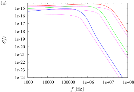
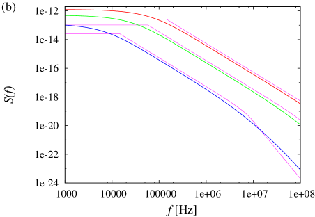
Figure 4: (Color online) Behavior of the integrated spectra of surface fluctuations $S(f)$ for (a) water and (b) oil with respect to $f$. The spectra are shown for $b=1,2.5,10\,[\mu$m^-1] (red, green, blue lines respectively), along with their analytic approximations (thin lines, magenta). The spectra for smaller $b$ have larger fluctuations across the spectrum.

IV Shot noise level

While our measurement precision is not limited by the shot noise of the probe laser beam, it is of import to understand how the shot noise level would appear in our setting. The electric current through the photodiode is $I=\kappa e{\cal P}/h\nu$, where ${\cal P}$ is the signal power, $e$ is the electron charge magnitude and $\kappa$ is the quantum efficiency of the photodiode. $\kappa\simeq 0.8$ for the photodiodes we use. The current generated by shot noise is

$$I_{\rm SN}=\sqrt{2eI\,\Delta f}=e\sqrt{{2\kappa{\cal P}\over h\nu}\Delta f}\qquad.$$ (20)

$\Delta f$ is the frequency range of the measurement. The signal in the experiment comes from difference in the current $\Delta I$ due to the geometric effects of the optical lever. For an inclination $\theta$, the signal is

$$\Delta I=\kappa{2e\theta{\cal P}\over h\nu N\!A}\qquad.$$ (21)

The shot noise level in our experiment is the size of the angular fluctuations $\theta^{2}_{\rm SN}$ corresponding to the shot noise current. This is what appears in the measurements, had we not used the noise reduction through correlations described in Sect. V. $\theta^{2}_{\rm SN}$ can be obtained from $\Delta I\simeq I_{\rm SN}$ to be

$$\theta_{\rm SN}^{2}\simeq{N\!A^{2}e\over 2I}\Delta f\qquad.$$ (22)

Here, the current $I$ is the photoelectric current collected by the dual photodiodes. $\theta_{\rm SN}^{2}$ is smaller for larger signals, which is natural. Also, for larger numerical apertures, the beam spot is focused down to a smaller size so that the effect of the optical lever is smaller, hence the shot noise effects are larger. In our experiment, $I\simeq 0.5\,\mu$A so that $\theta^{2}_{\rm SN}\simeq N\!A^{2}\times 1.6\times 10^{-13}\rm\,Hz^{-1}$. It is crucial to separate out the signal from this noise, using methods explained in the next section.

V Noise reduction through correlations

An essential feature of thermal fluctuations is that they are random. Since our objective is to directly measure the fluctuations under normal circumstances, the fluctuations are furthermore small. Even in ideally executed experiments, some random noise, such as shot noise, always exist. Therefore, to measure weak random signals, we need to separate out the random signal from the random noise. This is possible under rather general circumstances, as we now explainam1 . The principle behind this noise reduction is not limited to thermal fluctuations or optical measurements, but applies generally to the extraction of random signals from random noise. The conditions for its applicability will be discussed below.

A detector measurement $D_{1}=S+N_{1}$ consists of the desired signal $S$ and some noise $N_{1}$, independent of $S$. Denoting Fourier transforms with tildes, the power spectrum obtained under simple averaging is

$$\langle|\tilde{D}_{1}|^{2}\rangle=\langle|\tilde{S}|^{2}\rangle+\langle|\tilde{N}_{1}|^{2}\rangle\qquad.$$ (23)

Since the signal itself is random in nature, there is no way to distinguish the signal from the noise, so that the signal can not be measured, unless the signal is larger than the noise, $\langle|\tilde{S}|^{2}\rangle\gg\langle|\tilde{N}_{1}|^{2}\rangle$. If we use only one measurement, this is an essential limitation.

To overcome this obstacle, we make another independent measurement of the same signal, $D_{2}=S+N_{2}$, where $N_{2}$ denotes the noise for this measurement. Then,

$$\langle\overline{\tilde{D}_{1}}\tilde{D}_{2}\rangle\rightarrow\langle|\tilde{S}|^{2}\rangle\quad,\qquad{{\cal N}}\rightarrow\infty\qquad,$$ (24)

eliminating the random noise $N_{1},N_{2}$. Here $\cal N$ is the number of averagings. This results holds since the measurements $D_{1},D_{2}$ are independent and the cross-terms of decorrelated random observables (and their Fourier transforms) vanish under averaging. The relative error in this method is $\sim 1/\sqrt{{\cal N}}$, which arises from the statistical nature of the method. In principle, given enough averagings, we can suppress shot noise and other random noise effects to an arbitrarily small size.

The crucial requirements for our method to work is that multiple independent measurements can be made and that the signal is stable enough to withstand averagings. The independence of the measurements, or equivalently, the decorrelation of the noise in them is clearly crucial. As the signal becomes weaker, stricter independence is required, which in practice can be quite delicate. For instance, cross talks can arise in electronic circuits, unless they are completely separated and electronic signals can affect each other through electromagnetic fields in the intervening space. These properties put practical limitations on the reduced noise level. While our method can not be used for an one-time event, it can be used for any recurrent signal.

Another possible approach to reducing the relative noise is to increase the signal strength. In our context, this would mean increasing the beam intensity. However, this is not always applicable, since a stronger beam will affect the sample. Even for simple liquid surfaces, it leads to more evaporation and can lead to less precise measurements. More generally, if we consider biological materials or medical applicationsDenk , using a strong light source is often excluded. Correlation measurements have been used previously in surface light scattering experimentsEarnshaw . Our approach differs from those in that we use the cross-correlation of independent measurements of the same signal to reduce the noise.

VI Experimental results and theory

In Fig. 5, we compare the experimental results with the theory explained above for water, ethanol and oil with various beam sizes. The fluid properties we used for water, ethanol and oil are $(\rho\,{\rm[kg/m^{3}]},\sigma\,{\rm[kg/s^{2}]},\eta\,{\rm[kg/(m\cdot s)]})=(1.0\times 10^{3},7.3\times 10^{-2},1.0\times 10^{-3})$, $(0.79\times 10^{3},2.2\times 10^{-2},1.1\times 10^{-3})$ and $(0.92\times 10^{3},3.0\times 10^{-2},0.124)$, respectively. The agreement between the theoretical formula Eq. (11) and the experimental measurements is mostly quite satisfactory, including its beam size dependence. There is some excess signal in the water surface fluctuations at low frequencies for small $b$ (b=1.3 $\mu$m case in Fig. 5(a)), whose cause is explained below. The rough features of the spectra can be understood from Eqs. (18) and (19); the spectrum behaves as $S(f)\sim\eta/(\sigma^{2}b)$ at low frequencies. So, the fluctuations are the largest for oil due to its large viscosity and smallest for water due to its large surface tension. The fluctuations are larger for smaller $b$. At high frequencies, as we decrease $b$, the effective cutoff for the wavelength decreases and fluctuations at larger frequencies become more apparent.

The excess measurements in the water surface fluctuation spectrum at low frequencies for $b=1.3\,\mu$m can be explained as follows: Ideally, the experiment measures only inclination fluctuations of the surface. However, given the high sensitivity of the measurements, vertical displacements can mimic inclinations due to the focusing of the objective lens, when the beam alignment is not perfect. This effect is contained in $\langle|\tilde{a}_{0}(\omega)|^{2}\rangle$ which behaves as $\sim 1/f$ at low frequencies. For smaller $b$, this effect is larger due to the steeper focusing and can be seen in the water surface fluctuation measurements at low frequencies, since for a given beam size, $S(f)$ is smallest for water.

The shot noise levels in the measurements are $6\times 10^{-14},\ 3\times 10^{-14},2\times 10^{-15}\,[\rm Hz^{-1}]$ for the beam diameters $b=1.5,2.5,10\,[\mu$m], as explained in Sect. IV. Therefore, we see that the noise reduction using signal correlations explained in the previous section is crucial for examining even the qualitative features of the spectra, since most, and in some cases all, of the spectra is below shot noise levels.

Some comments regarding the calibration of the measurements is in order. On the theoretical side, given the properties of the liquid and the beam diameter, there are no further parameters at all in the spectrum Eq. (11) and is specified completely. Experimentally, the frequency dependence of the spectrum can be measured precisely. Calibrating the overall magnitude of the measured spectrum is more difficult and this is done using a piezoelectrically driven mirror with a known oscillation amplitude. While this works well when $b$ is large, for smaller $b$, the shallowness of the depth of field makes the calibration less accurate. Another complication is that the liquid in general evaporates during the measurement so that the beam defocuses. This, in effect, increases the beam diameter and can influence the spectral shape. This problem is clearly more acute for larger beam powers. A typical measurement of simple liquid surface fluctuations takes around 20 seconds and the beam power applied is $0.5\,$mW. Given the excellent agreement of the observed fluctuation spectra of simple liquid surfaces and theory, it might be reasonable to use thermal surface fluctuations of a well studied specific liquid such as oil to finely calibrate the system when applying the measurements to more general samples.

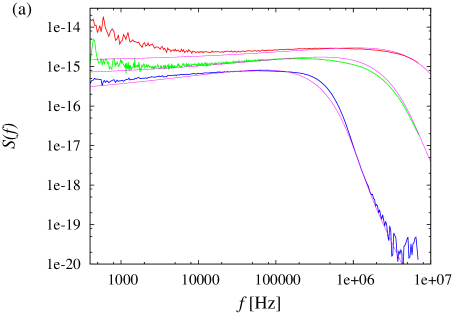
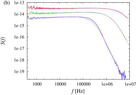
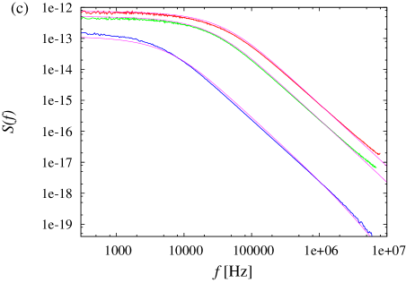
Figure 5: (Color online) Observed fluctuation spectra for (a) water ($b=1.3,3.1,11.5\,[\mu\rm m]$), (b) ethanol ($b=0.9,2.5,9.5\,[\mu\rm m]$) and (c) oil ($b=1.7,2.5,11.0\,[\mu\rm m]$), (red, green, blue lines from smaller to larger $b$). Respective theoretical spectra $S(f)$ are also shown (thin lines, magenta). The spectra for smaller $b$ have larger fluctuations.

In this work, we directly studied the spectra of thermal fluctuations for simple liquids, using surface light reflection methods. The spectra obtained are integrated over wavelengths and we have also investigated the dependence of the spectra on the beam diameter. In the process, we applied a novel general method for noise reduction, using the correlation of independent measurements of the same signal. The spectra obtained matches well with theory, whose analytic behavior can be summarized rather simply. The measurement method is complementary to the surface fluctuation measurements for specific wavelengths, when applied to simple liquids. The method, especially when combined with the noise reduction method, has a broad range of applicability since the required sample size, observation time and power are small.

References

- (1) M. von Schmoluchowski, Ann Physik 25, 225 (1908); L. Mandelstam, Ann. Physik 41, 609 (1913).
- (2) D. Langevin, “Light scattering by liquid surfaces and complementary techniques”, Marcel Dekker, New York (1992).
- (3) K. Numata, M. Ando, K. Yamamoto, S. Otsuka, K. Tsubono, Phys. Rev. Lett. 91, 260602 (2003); E.D. Black et al, Phys. Lett. A 328, 1 (2004)
- (4) H.J. Lauter et al, Phys. Rev. Lett 68, 2484 (1992); A. Vailati, M. Giglio, Nature 390, 262 (1997)
- (5) T. Mitsui, Jpn. J. Appl. Phys., 47, 6563 (2008)
- (6) A.Tay et al., Rev. Sci. Instrum. 79, 103107 (2008)
- (7) T. Mitsui, K. Aoki, Phys. Rev. DE 80, 020602(R)-1—4 (2009).
- (8) M.-A. Bouchiat, and J. Meunier, J. de Phys. 32, 561 (1971).
- (9) W. Denk and W. W. Webb, Appl. Opt. 29, 2382 (1990)
- (10) For instance, J.C. Earnshaw, Appl. Opt. 36, 7583 (1997).