On dark energy models of single scalar field

Abstract

In this paper we revisit the dynamical dark energy model building based on single scalar field involving higher derivative terms. By imposing a degenerate condition on the higher derivatives in curved spacetime, one can select the models which are free from the ghost mode and the equation of state is able to cross the cosmological constant boundary smoothly, dynamically violate the null energy condition. Generally the Lagrangian of this type of dark energy models depends on the second derivatives linearly. It behaves like an imperfect fluid, thus its cosmological perturbation theory needs to be generalized. We also study such a model with explicit form of degenerate Lagrangian and show that its equation of state may cross $-1$ without any instability.

PACS number(s): 98.80.Cq.

I Introduction

The recent data from type Ia Supernovae (SNIa) and cosmic microwave background (CMB) radiation and so on have provided strong evidences for a spatially flat and accelerated expanding universe. In the context of Friedmann-Robertson-Walker (FRW) cosmology with Einstein gravity, this acceleration is attributed to the domination of a component with negative pressure, called dark energy. So far, the nature of dark energy remains a mystery. Theoretically, the simplest candidate for such a component is a small positive cosmological constant, but it suffers the difficulties associated with the fine tuning and the coincidence problems. Therefore, many physicists are attracted by the idea of dynamical dark energy models, such as quintessence Ratra:1987rm ; Wetterich:1987fm ; Caldwell:1997ii , phantom Caldwell:1999ew , k-essence ArmendarizPicon:2000dh , quintom Feng:2004ad and so on (see Refs. Copeland:2006wr ; Frieman:2008sn ; Caldwell:2009ix ; Cai:2009zp ; Li:2011sd for recent reviews).

Although the recent fits to the data Li:2011dr , in combination of the 7-year WMAP Komatsu:2010fb , the Sloan Digital Sky Survey Reid:2009xm , and the recently released Union2 SNIa data Riess:2011yx , show remarkably the consistence of the cosmological constant, it is worth noting that a class of dynamical models with the equation-of-state (EoS) across $-1$, dubbed as quintom which dynamically violates the null energy condition (NEC), is mildly favored Feng:2004ad . However, it was noticed that consistent single field models realizing the quintom scenario are difficult to be constructed. For example, the EoS of quintessence is limited to be in the region $-1\leq w\leq 1$, while for phantom $w$ is always smaller than $-1$. It was proved that in models described by a single perfect fluid or a single scalar field with a Lagrangian of k-essence form ArmendarizPicon:1999rj , the cosmological perturbations encounter a divergence when the background EoS crosses $-1$ Feng:2004ad ; Vikman:2004dc ; Hu:2004kh ; Caldwell:2005ai ; Zhao:2005vj . This statement was explicitly proven in Ref. Xia:2007km as a “No-Go” theorem for dynamical dark energy models.

To realize a viable quintom scenario, one usually needs to add more degrees of freedom into the dark energy budget. The simplest and also the first quintom model was constructed by a combination of a canonical scalar and a phantom scalar field Feng:2004ad . However theorists are still interested in pursuing single field quintom models. The first single scalar field quintom model was realized by introducing higher order derivative terms Li:2005fm , also see Zhang:2006ck for generalization. It was also obtained in the frame of nonlocal string theory Aref'eva:2005fu and decaying tachyonic branes Cai:2007gs . However, there is a quantum instability due to an unbounded vacuum state in such type of models Carroll:2003st ; Cline:2003gs . A possible approach to stable violations of NEC is the ghost condensation of Ref. ArkaniHamed:2003uy , in which the negative kinetic modes are bounded via a spontaneous Lorentz symmetry breaking, although it might allow for superluminal propagation of information in some cases Dubovsky:2005xd . Various theoretical realizations of quintom scenarios and their implications for early universe physics were reviewed in Ref. Cai:2009zp (see also Qiu:2010ux ).

Recently, a scalar field model which stably violates the NEC has been studied extensively, which is the so-called Galileon Nicolis:2008in . It was viewed as a local infrared modification of General Relativity, generalizing an effective field description of the DGP model Dvali:2000hr . The key feature of these models is that they contain higher order derivative terms in the action while the equation of motion remains second-order in order to avoid the appearance of ghost modes, realizing the idea pioneered by Horndeski thirty years ago Horndeski:1974 . Later on, various phenomenological studies of this type of models were performed, namely, see Refs. deRham:2010eu ; Deffayet:2010qz ; Pujolas:2011he ; Deffayet:2009wt ; Deffayet:2011gz ; Gao:2011qe ; Chow:2009fm ; Silva:2009km ; DeFelice:2010pv ; Kobayashi:2010cm ; Hinterbichler:2010xn ; Creminelli:2010ba . Motivated by the feature of the Galileon model, in this paper we revisit quintom dark energy models containing higher derivative terms. We start from a general covariant Lagrangian of single scalar field involving higher derivative terms and pursue how to keep the model free from extra degree of freedom. We show that it is able to eliminate the ghost mode by imposing a degenerate condition that the Lagrangian only depends on the second derivative terms linearly. Based on the degenerate Lagrangian, we build an explicit dark energy model and study its dynamics of its homogeneous background and its perturbations. Our numerical calculations show that the EoS is able to cross the cosmological constant boundary smoothly and the perturbation modes are well controlled when the crossing takes place. We understand the reason of realizing the single field quintom without ghosts is that, such a single scalar field model is no longer be able to correspond to a perfect fluid. Thus, this model does not conflict with the “No-Go” theorem for quintom dark energy model building as proposed in Xia:2007km .

This paper is organized as follows. In Section II, we simply review the difficulty of constructing a single field dark energy model which gives rise to quintom scenario. In Section III, we start with a single field action involving higher derivative terms, and present the general analysis. We also discuss under what condition the higher derivative terms do not bring a ghost mode to the effective field description in Section IV. Section V is devoted to the study of the background and perturbation dynamics of single field dark energy model with degenerate higher derivatives in the frame of flat FRW universe. Specifically, we present an explicit model of quintom dark energy with degenerate higher derivatives. We perform numerical computation to illustrate such a model can realize the EoS across $-1$ smoothly. Section VI is the summary.

II The difficulty of single field dark energy models with EoS crossing $-1$

We begin by briefly reviewing the difficulty of constructing dynamical dark energy models with the EoS across the cosmological constant boundary. As demonstrated by several groups Feng:2004ad ; Vikman:2004dc ; Hu:2004kh ; Caldwell:2005ai ; Zhao:2005vj ; Xia:2007km , the EoS of dark energy based on single perfect fluid or single k-essence scalar field (quintessence and phantom are special cases of k-essence) cannot cross $-1$ remaining finite perturbations. The key point to the proof of this no-go theorem is that in both scenarios the pressure perturbation has a gauge invariant relation with energy and momentum density perturbations,

$$\delta p=c_{s}^{2}\delta\rho+3H(c_{s}^{2}-\frac{\dot{p}}{\dot{\rho}})\frac{V}{k^{2}}~{},$$ (1)

where the dot represents the derivative with respect to time, and $H=\dot{a}/a$ is the Hubble rate with $a$ the scale factor. The sound speed square $c_{s}^{2}$ is defined as the ratio of $\delta p/\delta\rho$ at the frame comoving with the dark energy, it should be positive definite to guarantee the Jeans stability of perturbations at small scales. The momentum density perturbation is defined as $V=ik^{i}T^{0}_{i}$ in Fourier space, here $T^{0}_{i}$ is the $0-i$ component of the energy momentum tensor. For perfect fluid the pressure is a function of the energy density only, $p=p(\rho)$, and $c_{s}^{2}=\dot{p}/\dot{\rho}$, hence $\delta p=(\dot{p}/\dot{\rho})\delta\rho$. For k-essence field the sound speed square is generally different from $\dot{p}/\dot{\rho}$, however, from Eq. (1) we can see that in both cases the pressure perturbation diverges at the crossing point $\dot{\rho}=0$ with finite $V$ and density perturbation. As we learn from the gravitational field equation, a divergent pressure perturbation will lead to arbitrarily large metric perturbations. This instability can also be seen from the equation of motion or the action for the perturbations. A generic form of Lagrangian for a k-essence field is only a function of the scalar $\phi$ and its first derivatives $X=\frac{1}{2}\nabla_{\mu}\phi\nabla^{\mu}\phi$, of which the action is expressed as,

$$S=\int d^{4}x\sqrt{g}\mathcal{L}(\phi,~{}X)~{},$$ (2)

where $g$ is the negative determinant of the metric tensor $g_{\mu\nu}$. Its energy momentum tensor has the same form as that of perfect fluid,

$$T^{\mu\nu}=-pg^{\mu\nu}+(\rho+p)u^{\mu}u^{\nu}~{},$$ (3)

where

$$p=\mathcal{L}~{},~{}~{}\rho=-p+2Xp_{X}~{},~{}~{}u^{\mu}=\frac{\nabla^{\mu}\phi}{\sqrt{2X}}~{}.$$ (4)

We have used the subscript $X$ to indicate the partial derivative with respect to $X$. The evolution of the k-essence perturbation $\pi=\phi(\vec{x},~{}t)-\phi(t)$ is governed by the equation which may be obtained via variational principle from the following action of second order,

$$S^{(2)}={1\over 2}\int d^{3}xdta^{3}[\rho_{X}\dot{\pi}^{2}-\frac{p_{X}}{a^{2}}\partial_{i}\pi\partial_{i}\pi+p_{\phi\phi}\pi^{2}-\frac{d(a^{3}\dot{\phi}p_{X\phi})/dt}{a^{3}}\pi^{2}]~{}.$$ (5)

We have neglected the metric perturbations for simplicity. We can see from the action that the sound speed square is $c_{s}^{2}=p_{X}/\rho_{X}$. However, from the relation $\rho+p=2Xp_{X}$ we know that $p_{X}$ vanishes at the point of crossing and changes the sign after the crossing. To guarantee $c_{s}^{2}>0$, $\rho_{X}$ should also vanish at the crossing point and change the sign afterwards, just as $p_{X}$. The vanishment of $\rho_{X}$ will make the equation of perturbation singular and the amplitude of the perturbation arbitrarily large around the crossing point.

Such kind of instability is classical. Another difficulty emerges when the quantum effects are considered. At the phantom phase $w<-1$, $p_{X}$ is negative and $c_{s}^{2}>0$ requires $\rho_{X}<0$. The action (5) showed that the kinetic term of $\pi$ has a wrong sign. This means $\pi$ in this phase is a ghost which brings the problem of vacuum instability due to the existence of negative energy states or of violating unitarity by negative norm states.

III Single scalar dark energy model with higher derivatives

To avoid the problem of singular perturbation possessed by single k-essence field, earlier quintom model buildings introduced multi-degree of freedom explicitly. For example in Ref.Feng:2004ad , the quintom model is constructed by a quintessence field and a phantom field. Though the total EoS of these two fields crosses $-1$ during the evolution, each component does not cross this boundary and has regular perturbation. Besides the multi-fluid or multi-field models, it is still interesting and important to pursue quintom models with single degree of freedom. To this end, some extensions beyond the perfect fluid and k-essence field are proposed in the literature including the higher derivative field theory Li:2005fm , the non-minimal coupling to the gravity Boisseau:2000pr , the constrained scalar field which violates Lorentz invariance locally Lim:2010yk , and so on. In this paper we only consider the first extension.

For a scalar field with higher (but finite) derivatives, its Lagrangian generally has the form,

$$\mathcal{L}=\mathcal{L}(\phi,\phi_{\mu_{1}},\phi_{\mu_{1}\mu_{2}},...,\phi_{\mu_{1}...\mu_{N}})~{},$$ (6)

where $\phi_{\mu_{1}}\equiv\nabla_{\mu_{1}}\phi,~{}\phi_{\mu_{1}\mu_{2}}\equiv\nabla_{\mu_{2}}\nabla_{\mu_{1}}\phi$ and so on are the covariant derivatives of $\phi$ and $N\geq 2$. The equation of motion from this Lagrangian is

$$\frac{\partial\mathcal{L}}{\partial\phi}+\sum_{n=1}^{N}(-1)^{n}\nabla_{\mu_{1}}...\nabla_{\mu_{n}}(\frac{\partial\mathcal{L}}{\partial\phi_{\mu_{1}...\mu_{n}}})=0~{}.$$ (7)

Generally this is a $2N$th order derivative equation, the whole system contains $N$ degrees of freedom and some of them are ghosts. In order to keep the discussions simple and without loss of general properties of higher derivative field theories, we only consider the case $N=2$ in curved spacetime, the Lagrangian is a scalar function of $\phi,~{}\phi_{\mu}$ and $\phi_{\mu\nu}$. The equation of motion is

$$\frac{\partial\mathcal{L}}{\partial\phi}-\nabla_{\mu}(\frac{\partial\mathcal{L}}{\partial\phi_{\mu}})+\nabla_{\mu}\nabla_{\nu}(\frac{\partial\mathcal{L}}{\partial\phi_{\mu\nu}})=0~{}.$$ (8)

Expanding this equation and considering the symmetry $\phi_{\mu\nu}=\phi_{\nu\mu}$, we have the following equation,

$$\frac{\partial\mathcal{L}}{\partial\phi}-\frac{\partial^{2}\mathcal{L}}{\partial\phi\partial\phi_{\mu}}\phi_{\mu}+(\frac{\partial^{2}\mathcal{L}}{\partial\phi\partial\phi_{\mu\nu}}-\frac{\partial^{2}\mathcal{L}}{\partial\phi_{\nu}\partial\phi_{\mu}})\phi_{\nu\mu}+\frac{\partial^{3}\mathcal{L}}{\partial\phi\partial\phi\partial\phi_{\mu\nu}}\phi_{\mu}\phi_{\nu}+2\frac{\partial^{3}\mathcal{L}}{\partial\phi\partial\phi_{\rho}\partial\phi_{\mu\nu}}\phi_{\rho\mu}\phi_{\nu}+\frac{\partial^{3}\mathcal{L}}{\partial\phi_{\rho}\partial\phi_{\sigma}\partial\phi_{\mu\nu}}\phi_{\sigma\mu}\phi_{\rho\nu}+$$

$$\frac{\partial^{2}\mathcal{L}}{\partial\phi_{\rho}\partial\phi_{\mu\nu}}(\phi_{\nu\rho\mu}-\phi_{\nu\mu\rho})+2\frac{\partial^{3}\mathcal{L}}{\partial\phi\partial\phi_{\rho\sigma}\partial\phi_{\mu\nu}}\phi_{\rho\sigma\mu}\phi_{\nu}+2\frac{\partial^{3}\mathcal{L}}{\partial\phi_{\alpha}\partial\phi_{\rho\sigma}\partial\phi_{\mu\nu}}\phi_{\rho\sigma\mu}\phi_{\alpha\nu}+\frac{\partial^{3}\mathcal{L}}{\partial\phi_{\alpha\beta}\partial\phi_{\rho\sigma}\partial\phi_{\mu\nu}}\phi_{\alpha\beta\mu}\phi_{\rho\sigma\nu}+$$

$$\frac{\partial^{2}\mathcal{L}}{\partial\phi_{\rho\sigma}\partial\phi_{\mu\nu}}\phi_{\rho\sigma\nu\mu}=0~{}.$$ (9)

If the matrix $\frac{\partial^{2}\mathcal{L}}{\partial\phi_{\rho\sigma}\partial\phi_{\mu\nu}}$ is non-degenerate, this is a fourth order differential equation. To solve this equation we need to impose the values of $\phi,~{}\phi_{\mu},~{}\phi_{\mu\nu},~{}\phi_{\mu\nu\rho}$ at the initial surface. This means such a model essentially possesses two dynamical components.

The first dark energy model of single scalar field with higher derivatives was proposed in Li:2005fm where a simple example is taken to illustrate the feature of crossing the boundary of $-1$. The sample model has the Lagrangian of the type,

$$\mathcal{L}=AX+B(\Box\phi)^{2}-V(\phi)~{},$$ (10)

where $\Box=\nabla_{\mu}\nabla^{\mu}$, $V(\phi)$ is the potential and $A,~{}B$ are constants. In Ref. Li:2005fm , it was shown explicitly that this model is equivalent to the double-field model with lower derivatives, but one field has negative kinetic term. This can be shown as follows. Taking an integration by parts the Lagrangian (10) can be rewritten as a function which does not depend on $X$. So it belongs to the more general class in which the Lagrangian is an arbitrary scalar function of $\phi$ and $\Box\phi$,

$$\mathcal{L}=\mathcal{L}(\phi,~{}\Box\phi)~{}.$$ (11)

Now we use this Lagrangian to illustrate how is the non-degenerate higher derivative field model equivalent to multi-field model with lower derivatives. Non-degeneracy means $\mathcal{L}_{BB}\neq 0$, where the subscript $B$ represents the derivative with respect to $\Box\phi$. We first introduce an auxiliary field defined as

$$\varphi\equiv\mathcal{L}_{B}~{}.$$ (12)

Due to the non-degeneracy, we may convert the above equation to get $\Box\phi$ as a function of $\phi$ and $\varphi$. Then change the independent variables $(\Box\phi,~{}\phi)$ to $(\phi,~{}\varphi)$, we accordingly have the Legendre transform of the Lagrangian in Eq. (11),

$$U(\phi,~{}\varphi)=\phi\Box\phi(\phi,~{}\varphi)-\mathcal{L}~{},$$ (13)

it may be considered as a potential of $\phi$ and $\varphi$. After finding the potential $U$, the higher derivative term in the Lagrangian (11) can be removed with the price of introducing extra field,

$$\mathcal{L}=\varphi\Box\phi-U(\phi,~{}\varphi)~{},$$ (14)

which is equivalent to the following Lagrangian

$$\mathcal{L}^{\prime}=-\nabla_{\mu}\varphi\nabla^{\mu}\phi-U(\phi,~{}\varphi)~{}.$$ (15)

This equivalent Lagrangian has a more clear form of double fields,

$$\mathcal{L}^{\prime}=\frac{1}{2}\nabla_{\mu}\phi_{1}\nabla^{\mu}\phi_{1}-\frac{1}{2}\nabla_{\mu}\phi_{2}\nabla^{\mu}\phi_{2}-U(\phi_{1},~{}\phi_{2})~{},$$ (16)

through the field redefinitions

$$\phi_{1}=\frac{1}{\sqrt{2}}(\phi-\varphi)~{},~{}~{}~{}~{}\phi_{2}=\frac{1}{\sqrt{2}}(\phi+\varphi)~{}.$$ (17)

The mode $\phi_{2}$ is a ghost which violates the null energy condition because its kinetic term has a wrong sign. This explains why the model (11) may cross the cosmological constant boundary without divergent perturbation. However at the quantum level, the non-degenerate higher derivative model is plagued by the existence of ghost mode.

IV Degenerate higher derivative model

In the degenerate higher derivative model, the matrix $\frac{\partial^{2}\mathcal{L}}{\partial\phi_{\rho\sigma}\partial\phi_{\mu\nu}}$ in Eq. (III) is identically zero. Correspondingly, all the third and fourth order derivative terms in the equation of motion (III) disappear, i.e.,

$$\frac{\partial\mathcal{L}}{\partial\phi}-\frac{\partial^{2}\mathcal{L}}{\partial\phi\partial\phi_{\mu}}\phi_{\mu}+(\frac{\partial^{2}\mathcal{L}}{\partial\phi\partial\phi_{\mu\nu}}-\frac{\partial^{2}\mathcal{L}}{\partial\phi_{\nu}\partial\phi_{\mu}})\phi_{\nu\mu}+\frac{\partial^{3}\mathcal{L}}{\partial\phi\partial\phi\partial\phi_{\mu\nu}}\phi_{\mu}\phi_{\nu}+2\frac{\partial^{3}\mathcal{L}}{\partial\phi\partial\phi_{\rho}\partial\phi_{\mu\nu}}\phi_{\rho\mu}\phi_{\nu}+\frac{\partial^{3}\mathcal{L}}{\partial\phi_{\rho}\partial\phi_{\sigma}\partial\phi_{\mu\nu}}\phi_{\sigma\mu}\phi_{\rho\nu}+$$

$$\frac{\partial^{2}\mathcal{L}}{\partial\phi_{\rho}\partial\phi_{\mu\nu}}\phi_{\sigma}R^{\sigma}_{~{}~{}\nu\mu\rho}=0~{},$$ (18)

where we have used the commutation of the covariant derivatives $\phi_{\nu\rho\mu}-\phi_{\nu\mu\rho}=\phi_{\sigma}R^{\sigma}_{~{}~{}\nu\mu\rho}$ with $R^{\sigma}_{~{}~{}\nu\mu\rho}$ the Riemann tensor. The equation of motion remains to be a second order differential equation, but there is a curvature-field coupling term appeared in it even though we only consider the minimal coupling to the gravity in the Lagrangian. This means the degenerate model has no extra degree of freedom.

Zero matrix $\frac{\partial^{2}\mathcal{L}}{\partial\phi_{\rho\sigma}\partial\phi_{\mu\nu}}$ implies the Lagrangian only depends on the second derivative terms linearly. With Lorentz invariance, $\mathcal{L}$ can only be

$$\mathcal{L}=K(\phi,~{}X)+G(\phi,~{}X)\Box\phi+F(\phi,~{}X)\nabla^{\mu}\phi\nabla^{\nu}\phi\nabla_{\mu}\nabla_{\nu}\phi~{}.$$ (19)

The box term at the right hand side with $G=X$ was considered in the context of Galileon theory Nicolis:2008in and its generalization was studied in Deffayet:2010qz , named as $KGB$ model and in inflation model building Kobayashi:2010cm , named as $G$-inflation. The box term is equivalent to $-2XG_{\phi}-G_{X}\nabla^{\mu}\phi\nabla^{\nu}\phi\nabla_{\mu}\nabla_{\nu}\phi$ after integration by parts and dropping a surface term. By redefinitions of $K(\phi,~{}X)$ and $F(\phi~{},X)$, the degenerate Lagrangian may be generally written as

$$\mathcal{L}=K(\phi,~{}X)+F(\phi,~{}X)\nabla^{\mu}\phi\nabla^{\nu}\phi\nabla_{\mu}\nabla_{\nu}\phi=K+F\nabla_{\mu}X\nabla^{\mu}\phi~{}.$$ (20)

Now we will investigate whether the dark energy model from this Lagrangian can stably cross the boundary of cosmological constant by studying its background evolution and properties of perturbations.

With the notations (20) the equation of motion (IV) becomes

$$K_{\phi}-2XK_{X\phi}-K_{X}\Box\phi-K_{XX}\nabla_{\mu}X\nabla^{\mu}\phi+F[(\Box\phi)^{2}-\nabla_{\mu}\nabla_{\nu}\phi\nabla^{\mu}\nabla^{\nu}\phi+R_{\mu\nu}\nabla^{\mu}\phi\nabla^{\nu}\phi]$$ (21)

$$+ 2F_{\phi}(\nabla_{\mu}X\nabla^{\mu}\phi+2X\Box\phi)+2XF_{\phi X}\nabla_{\mu}X\nabla^{\mu}\phi+4X^{2}F_{\phi\phi}+F_{X}(\Box\phi\nabla_{\mu}X\nabla^{\mu}\phi-\nabla_{\mu}X\nabla^{\mu}X)=0~{}.$$

The energy momentum tensor which sources the gravitational field is obtained through the variation of the action with respect to the metric tensor,

$$T^{\mu\nu}=-\frac{2}{\sqrt{g}}\frac{\delta S}{\delta g_{\mu\nu}}~{},$$ (22)

for the degenerate model it is

$$T^{\mu\nu}=-(K+F\nabla_{\rho}X\nabla^{\rho}\phi)g^{\mu\nu}+(K_{X}-2XF_{\phi}-F\Box\phi)\nabla^{\mu}\phi\nabla^{\nu}\phi+F(\nabla^{\mu}X\nabla^{\nu}\phi+\nabla^{\nu}X\nabla^{\mu}\phi)~{}.$$ (23)

We can read off the pressure and energy density from this energy momentum tensor up to linear order of perturbations around the homogeneous background,

$$p = K+F\nabla_{\mu}X\nabla^{\mu}\phi~{},$$ (24)

$$\rho = -K+F\nabla_{\mu}X\nabla^{\mu}\phi+2X(K_{X}-2XF_{\phi}-F\Box\phi)~{}.$$ (25)

In terms of the fluid variables $p$ and $\rho$, the energy momentum tensor may be rewritten as

$$T^{\mu\nu}=-pg^{\mu\nu}+(\rho+p)u^{\mu}u^{\nu}+(2X)^{3/2}F(a^{\mu}u^{\nu}+a^{\nu}u^{\mu})~{},$$ (26)

where by analogy with k-inflation Garriga:1999vw or k-essence ArmendarizPicon:2000dh we have defined the four velocity $u^{\mu}=\nabla^{\mu}\phi/\sqrt{2X}$ which is normalized as $u^{\mu}u_{\mu}=1$, $a^{\mu}\equiv u^{\rho}\nabla_{\rho}u^{\mu}$ is the four acceleration which is orthogonal to the velocity, i.e., $a_{\mu}u^{\mu}=0$. We have also used the relation Pujolas:2011he :

$$\nabla^{\mu}X=2Xa^{\mu}+u^{\rho}\nabla_{\rho}Xu^{\mu}~{}.$$ (27)

This energy momentum tensor (26) does not have the form of perfect fluid due to the last two terms depending on the four acceleration. In the language of relativistic imperfect fluid, $a^{\mu}$ can be identified as heat flow. Further, one can prove straitforwardly that $a^{\mu}$ is space like and its zero-th component vanishes at both background and linear levels, its spatial components $a_{i}$ should be first order variables. So if we redefine the four velocities as

$$\tilde{u}^{\mu}=u^{\mu}+\frac{(2X)^{3/2}F}{\rho+p}a^{\mu}~{},$$ (28)

the energy-momentum tensor should be

$$T^{\mu\nu}=-pg^{\mu\nu}+(\rho+p)\tilde{u}^{\mu}\tilde{u}^{\nu}-\frac{(2X)^{3}F^{2}}{\rho+p}a^{\mu}a^{\nu}\simeq-pg^{\mu\nu}+(\rho+p)\tilde{u}^{\mu}\tilde{u}^{\nu}~{}.$$ (29)

In the last step, we have considered the fact that the product $a^{\mu}a^{\nu}$ is a second order variable and can be neglected if we restrict our studies on the background evolution and the linear perturbation theory. This equation means the energy momentum tensor of the degenerate model has apparently the same form of perfect fluid if we neglect perturbations of higher order. But it is essentially different from perfect fluid, especially the relation (1) between the pressure and density perturbations is lost in this model. This is the very reason why the degenerate higher derivative model is possible to realize the quintom idea and avoid the problems possessed by single k-essence field.

V Cosmology with degenerate higher derivative dark energy model

In this section, we consider in more detail the dynamics of the dark energy model (20). The background universe is a spatially flat FRW spacetime, in which the metric is given by

$$ds^{2}=dt^{2}-a^{2}(t)\delta_{ij}dx^{i}dx^{j}~{}.$$ (30)

At the background level the field $\phi$ is homogeneous, so we soon have

$$\rho=-K+2X(K_{X}-2XF_{\phi}-3H\dot{\phi}F)$$

$$p=K+2X\ddot{\phi}F$$

$$\rho+p=2X(K_{X}-2XF_{\phi}-3H\dot{\phi}F+\ddot{\phi}F)~{},$$ (31)

where we have considered $X=\dot{\phi}^{2}/2~{},\nabla_{\mu}X\nabla^{\mu}\phi=2X\ddot{\phi}$ and $\Box\phi=\ddot{\phi}+3H\dot{\phi}$. The energy conservation law in the expanding universe $\dot{\rho}+3H(\rho+p)=0$ is identical to the equation of motion (21). For the velocity $u^{\mu}$ only the time component is non-zero, $u^{0}=1,~{}u^{i}=0$. The key point for this model to cross the cosmological constant boundary is that $K_{X}-2XF_{\phi}-3H\dot{\phi}F+\ddot{\phi}F$ could evolve from the positive region to the negative region or vise versa providing the energy density always positive. In addition, we have to check whether the perturbations are stable.

Similar to the analysis in single k-essence model, the perturbation of the scalar field is a small deviation from the homogenous background

$$\phi(\vec{x},~{}t)=\phi(t)+\pi(\vec{x},~{}t)~{}.$$ (32)

For complete consideration we should also include the perturbations of spacetime. However, for dark energy, it is believed to be subdominant in the universe for most time and had tiny contribution to the curvature. So for studying the dark energy perturbations, it is safely to neglect the metric perturbations which are sourced mainly by other matter. This approximation will greatly simplify the analysis. There are two ways to get the linear perturbation equations. One is to directly perturb the equation of motion (21) around the background evolution. Another one is to adapt the variational principle from the action which is second order of perturbations as we have shown in Sec. II for k-essence field. Here we will use the second way to discuss the perturbation of the scalar field. For this purpose we firstly expand the action

$$S=\int d^{4}x\sqrt{g}(K+F\nabla_{\mu}X\nabla^{\mu}\phi)$$ (33)

to the second order of the perturbations. After straightforward but tedious calculations, we obtain the desired second order action for $\pi$,

$$S^{(2)}(\pi) = {1\over 2}\int d^{3}xdta^{3}(A\dot{\pi}^{2}-\frac{B}{a^{2}}\partial_{i}\pi\partial_{i}\pi+C\pi^{2})~{},$$ (34)

with

$$A = K_{X}+2XK_{XX}-6H\dot{\phi}(F+XF_{X})-8XF_{\phi}-4X^{2}F_{X\phi}~{},$$

$$B = K_{X}-2(\ddot{\phi}+2H\dot{\phi})F-4XF_{\phi}-2X\ddot{\phi}F_{X}~{},$$

$$C = \frac{d}{dt}(6HXF_{\phi}+2X\dot{\phi}F_{\phi\phi}-\dot{\phi}K_{X\phi})+3H(6HXF_{\phi}+2X\dot{\phi}F_{\phi\phi}-\dot{\phi}K_{X\phi})+2X\ddot{\phi}F_{\phi\phi}+K_{\phi\phi}~{}.$$ (35)

We can see from the action that the sound speed square is defined as

$$c_{s}^{2}=\frac{B}{A}=\frac{K_{X}-2(\ddot{\phi}+2H\dot{\phi})F-4XF_{\phi}-2X\ddot{\phi}F_{X}}{K_{X}+2XK_{XX}-6H\dot{\phi}(F+XF_{X})-8XF_{\phi}-4X^{2}F_{X\phi}}~{}.$$ (36)

If the universe is dominated by the scalar field, as discussed in the $KGB$ model Deffayet:2010qz or the $G$-inflation model Kobayashi:2010cm , a full treatment of the gravity-$\phi$ coupled system based on the (Arnowitt-Deser-Misner) ADM method will give a slightly different sound speed squared,

$$c_{s}^{\prime 2}=\frac{K_{X}-2(\ddot{\phi}+2H\dot{\phi})F-4XF_{\phi}-2X\ddot{\phi}F_{X}-2X^{2}F^{2}/M_{p}^{2}}{K_{X}+2XK_{XX}-6H\dot{\phi}(F+XF_{X})-8XF_{\phi}-4X^{2}F_{X\phi}+6X^{2}F^{2}/M_{p}^{2}}~{},$$ (37)

where both numerator and denominator are modified by terms suppressed by the Planck mass $M_{p}^{2}=1/8\pi G$. This sound speed depends on the gravity theory, here the gravity theory is Einstein’s general relativity. For dark energy studied in this paper we will consider the sound speed in Eq. (36) to express the propagating velocity of the perturbations.

The classical stability requires $c_{s}^{2}>0$. Furthermore, the absence of ghost mode corresponds to

$$A=K_{X}+2XK_{XX}-6H\dot{\phi}(F+XF_{X})-8XF_{\phi}-4X^{2}F_{X\phi}>0~{}.$$ (38)

Compared to Eq. (V) one can find that neither $A$ nor $B$ is proportional to $\rho+p$, hence when the dark energy crosses the cosmological constant boundary, $\rho+p=0$, both coefficients $A$ and $B$ are not vanished in general. The equation of motion would be regular at the crossing point. This is different from the case of k-essence model discussed in Section II. So in this single field model, for particular choices of the functions $K$ and $F$ and corresponding model parameters, it is possible to find solutions in which the equation of state of dark energy evolves across $-1$ but both $c_{s}^{2}$ and $A$ remain finite and positive as we will show explicitly below. Within these solutions the fluctuation of the scalar field has the right kinetic term to circumvent the pathology of ghost, even though its background part has $w<-1$ violating the null energy condition.

In order to illustrate the realization of quintom scenario explicitly, we study an explicit form of the degenerate dark energy model. The Lagrangian we are considering is simple:

$$\mathcal{L}=-X-c_{1}\nabla_{\mu}X\nabla^{\mu}\phi+c_{2}X\phi^{2}~{},$$ (39)

where $c_{1,2}$ are constants. Compared with the notations in Eq. (20), one may find that $K=-X+c_{2}X\phi^{2}$ and $F=-c_{1}$. Note that the third term can also be viewed as an “effective mass term”. From Eqs. (24) and (25), we get the pressure and energy density of this model respectively as:

$$\rho = (c_{2}\phi^{2}-1+6c_{1}H\dot{\phi})X~{},$$ (40)

$$p = (c_{2}\phi^{2}-1-2c_{1}\ddot{\phi})X~{}.$$ (41)

At the point where the equation of state crossing $-1$, we have $\rho+p=0$, i.e.,

$$c_{1}(\ddot{\phi}-3H\dot{\phi})=c_{2}\phi^{2}-1~{}.$$ (42)

In addition, we have the equation of motion for the scalar field, which comes from Eq. (21),

$$(1-6c_{1}H\dot{\phi}-c_{2}\phi^{2})\ddot{\phi}+3H(1-c_{2}\phi^{2})\dot{\phi}-(c_{2}\phi+9c_{1}H^{2}+3c_{1}\dot{H})\dot{\phi}^{2}=0~{}.$$ (43)

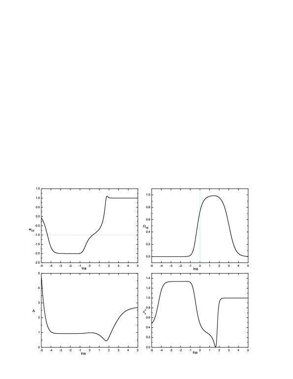
Figure 2: The equation of state $w_{DE}$, the energy density ratio $\Omega_{DE}$, parameter $A$ and sound speed squared $c_{s}^{2}$ of dark energy of the model (39). The parameters are chosen to be $c_{1}=3.0\times 10^{122}$, $c_{2}=0.05$ and the initial conditions are chosen in the far past when the universe was matter dominated. The equation of sate crosses $-1$ recently, and becomes larger than $0$ in the future. Both $A$ and $c_{s}^{2}$ are positive during the evolution. The universe will be matter-dominant in the future.

We performed the numerical calculations of the background evolution and the coefficients for perturbations for different parameter choices in Figs. 1 and 2. In both figures, we have used the unit $8\pi G=1$ and chose the parameter $c_{1}=3.0\times 10^{122}$. The choices of parameter $c_{2}$ are different for these two cases. In the first figure $c_{2}=0$ and in the second one $c_{2}=0.05$. In both cases we set the initial conditions as $\phi_{i}=-1.2$ and $\dot{\phi}_{i}=10^{-61}$ well within the matter dominated era in order to make the evolutions of dark energy consistent with the observations. We can see that in both cases the equation of state of dark energy crosses the cosmological constant boundary, and the present values of $w_{DE}$ and $\Omega_{DE}$ fits well with the observational data. At present time $\ln a=0$, $w_{DE}=-1.158$ and $-1.167$ for the first and second cases respectively. These are consistent with the current constraint by the observational data from CMB, LSS and Supernovae. For example the analysis in Ref. Liu:2010ba gives $w_{DE}=-1.143\pm 0.160$. The values of $\Omega_{DE}$ in both cases are around $0.725$, also compatible with the observations Komatsu:2010fb . Moreover, the parameter $A$ defined in (V) and the sound speed squared defined in (36) are both positive during evolutions in these two cases. This means that at the crossing there is no ghost instability and the perturbation is regular and classically stable.

Finally we should emphasize that with different parameters, these two cases give rise to predictions of different fate of dark energy in the future. For the first case where $c_{2}=0$ which reduces to the case discussed in Deffayet:2010qz , $w_{DE}$ crosses $-1$ and approaches $-2$ at early time, then when the dark energy dominates the universe $w_{DE}$ will approach to $-1$ forever and the universe enters into the De Sitter phase. This can be understood as follows. With vanished $c_{2}$, the model is symmetric under the field shift $\phi\rightarrow\phi+C$ with constant $C$. The corresponding Noether current is

$$J^{\mu}=c_{1}\nabla^{\mu}X+\nabla^{\mu}\phi-c_{1}\Box\phi\nabla^{\mu}\phi~{},$$ (44)

and the conservation law $\nabla_{\mu}J^{\mu}=0$ is nothing but the equation of motion. For the background, $\phi$ is homogeneous the conservation law simplifies as

$$\dot{J}^{0}+3HJ^{0}=0~{},$$ (45)

and the “charge density” $J^{0}=\dot{\phi}-3c_{1}H\dot{\phi}^{2}$, which scales as $a^{-3}$. From it we can solve for $\dot{\phi}$ that

$$\dot{\phi}=\frac{1\pm\sqrt{1-12c_{1}HJ^{0}}}{6c_{1}H}~{}.$$ (46)

On the other hand the energy density and pressure are respectively

$$\rho = (-1+6c_{1}H\dot{\phi})\frac{\dot{\phi}^{2}}{2}$$

$$p = -(1+2c_{1}\ddot{\phi})\frac{\dot{\phi}^{2}}{2}~{}.$$ (47)

To guarantee the positivity of the energy density, $6c_{1}H\dot{\phi}>1$, in Eq. (46), we should choose the plus sign, i.e.,

$$\dot{\phi}=\frac{1+\sqrt{1-12c_{1}HJ^{0}}}{6c_{1}H}~{}.$$ (48)

Because $J^{0}$ scales as $a^{-3}$, soon after the beginning $J^{0}$ approaches to zero so that $\dot{\phi}\rightarrow\frac{1}{3c_{1}H}$ and $\ddot{\phi}\rightarrow-\frac{\dot{H}}{3c_{1}H^{2}}$. This time the universe is still dominated by matter and the Hubble rate $H$ scales as $a^{-3/2}$, it is easy to obtain that $\ddot{\phi}$ approaches to the constant $\frac{1}{2c_{1}}$. So the equation of state

$$w_{DE}=-\frac{1+2c_{1}\ddot{\phi}}{-1+6c_{1}H\dot{\phi}}\rightarrow-(1+2c_{1}\ddot{\phi})=-2~{}.$$ (49)

This is a phantom attractor solution to the model. At this period, the energy density of the dark energy increases as fast as $a^{3}$ and the matter energy density decreases as $a^{-3}$. So with the initial conditions we have chosen the universe transits to the phase of dark energy domination at low redshift. In this phase $\dot{\phi}$ is more close to $\frac{1}{3c_{1}H}$ than in the matter dominated era. However, the Hubble rate is

$$H^{2}\simeq{1\over 3}(-1+6c_{1}H\dot{\phi})\frac{\dot{\phi}^{2}}{2}\rightarrow\frac{\dot{\phi}^{2}}{6}\rightarrow\frac{1}{54c_{1}^{2}H^{2}}~{},$$ (50)

so $H$ approaches to the constant $(54c_{1}^{2})^{-1/4}$ and $\ddot{\phi}\rightarrow 0$. The equation of state $w_{DE}\rightarrow-(1+2c_{1}\ddot{\phi})\rightarrow-1$. The universe enters into the de Sitter phase in the future.

For the second case where $c_{2}=0.05$, the shift symmetry is violated by the “effective” mass term. The “charge density” satisfies the equation

$$\dot{J}^{0}+3HJ^{0}=-c_{2}\dot{\phi}^{2}\phi~{},$$ (51)

where the density $J^{0}$ gets a minor modification compared with the first case,

$$J^{0}=(1-c_{2}\phi^{2})\dot{\phi}-3c_{1}H\dot{\phi}^{2}~{}.$$ (52)

With the parameters and the initial conditions we have chosen, the effective mass term is very small at the time of matter domination. The early evolution of dark energy in this case is similar to the first case, its equation of state crosses $-1$ and approaches to the phantom attractor solution $w_{DE}=-2$. Because the initial value of $\phi$ we have chosen is negative and $\dot{\phi}\simeq\frac{1}{3c_{1}H}>0$, $\phi$ increases from the negative region to the positive one, so the effective mass term remains small during a fairly long period. Recently when the universe shifts to the dark energy dominated phase, $w_{DE}$ increases from $-2$ and approaches $-1$. However, the value of the field $\phi$ increases continually and the effective mass term becomes more and more important. So the universe will not enter into the de Sitter phase and $w_{DE}$ increases continually and gets back to larger than zero again. When $c_{2}\phi^{2}$ increases to the value much larger than unity, it will dominate the energy density and the pressure of the dark energy as seen from Eq. (40). The equation of state $w_{DE}\rightarrow 1$, but this phase is not stable because the energy density of the dark energy will decrease as fast as $a^{-6}$. Hence in the future dark energy might exit domination and the universe will return to matter-dominant stage. This phenomenon of the model has not been discussed before.

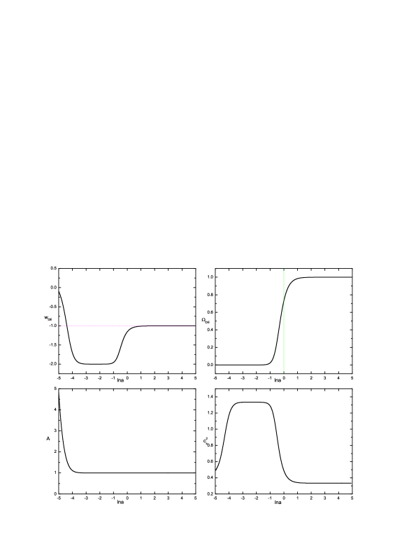
Figure 1: The equation of state $w_{DE}$, the energy density ratio $\Omega_{DE}$, parameter $A$ and sound speed squared $c_{s}^{2}$ of dark energy of the model (39). The parameters are chosen to be $c_{1}=3.0\times 10^{122}$, $c_{2}=0$ and the initial conditions are chosen in the far past when the universe was matter dominated. The equation of sate crosses $-1$ recently, and approach to $-1$ in the future. Both $A$ and $c_{s}^{2}$ are positive during the evolution. The universe will be dark energy dominant in the future.

VI Summary

The model building of dark energy which is possible to cross the cosmological constant boundary, i.e., the quintom dark energy has attracted a lot of attention in the literature (for example see Refs. Quintom_sum ). A very interesting question is how to build a single scalar model which gives rise to the crossing without any instabilities. The past studies have shown that a single scalar field satisfying a generic k-essence Lagrangian cannot give rise to the stable violation of NEC. However, it becomes possible when higher derivative operators are introduced. The non-degenerate higher derivative model can eliminate the classical instabilities but is still plagued by the ghost mode. In this paper we considered the degenerate higher derivative model inspired by the Galileon theory and its generalizations. We started with a single scalar of which the Lagrangian contains generic higher derivative operator, and then suggested a degenerate condition to eliminate the extra degrees of freedom brought by these higher derivative operators. Using the degenerate condition in the curved spacetime, the Lagrangian can be reduced to the form (20). We studied the cosmological application of this model, including the background and perturbation analysis. Particularly, we chose an explicit example and performed a detailed numerical computation. Our numerical results verified that this model is able to realize the EoS to cross the cosmological constant boundary and the perturbation evolves smoothly without any pathologies.

A quintom model which successfully violates the NEC without leading to quantum instability also has important implications to the early universe physics. In Refs. Cai:2007 , the authors found that a quintom model can avoid the big bang singularity widely existing in standard and inflationary cosmologies. In this picture, the moment of initial singularity can be replaced by a big bounce. Based on this scenario, the corresponding perturbation theory has been extensively developed, namely, on adiabatic perturbations Cai:2008qb ; Cai:2008qw ; Cai:2009hc , non-GaussianitiesCai:2009fn , entropy fluctuationsCai:2008qw ; Cai:2011zx , and the related preheating phaseCai:2011ci . Recently, it was observed that the Galileon model with the EoS across $-1$ exactly leads to a bouncing solution in the frame of the flat FRW universeQiu:2011cy . Consequently, we expect that bouncing cosmologies can be realized in a generic quintom model with degenerate higher derivative operators.

VII Acknowledgement

The research of ML is supported in part by National Science Foundation of China under Grants No. 11075074 and No. 11065004, by the Specialized Research Fund for the Doctoral Program of Higher Education (SRFDP) under Grant No. 20090091120054 and by SRF for ROCS, SEM. TQ is supported by Taiwan National Science Council (NSC) under Project No. NSC98-2811-M-002-501 and No. NSC98-2119-M-002-001. YC is supported by funds of physics department at Arizona State University. XZ is supported in part by the National Science Foundation of China under Grants No. 10821063, 10975142 and 11033005, and by the Chinese Academy of Sciences under Grant No. KJCX3-SYW-N2.

References

- (1) B. Ratra and P. J. E. Peebles, Phys. Rev. D 37, 3406 (1988).
- (2) C. Wetterich, Nucl. Phys. B 302, 668 (1988).
- (3) R. R. Caldwell, R. Dave and P. J. Steinhardt, Phys. Rev. Lett. 80, 1582 (1998) [arXiv:astro-ph/9708069].
- (4) R. R. Caldwell, Phys. Lett. B 545, 23 (2002) [arXiv:astro-ph/9908168].
-
(5)
T. Chiba, T. Okabe and M. Yamaguchi,
Phys. Rev. D 62, 023511 (2000)
[arXiv:astro-ph/9912463];
C. Armendariz-Picon, V. F. Mukhanov, P. J. Steinhardt, Phys. Rev. Lett. 85, 4438 (2000) [arXiv:astro-ph/0004134]. - (6) B. Feng, X. L. Wang and X. M. Zhang, Phys. Lett. B 607, 35 (2005) [arXiv:astro-ph/0404224].
- (7) E. J. Copeland, M. Sami and S. Tsujikawa, Int. J. Mod. Phys. D 15, 1753 (2006) [arXiv:hep-th/0603057].
- (8) J. Frieman, M. Turner and D. Huterer, Ann. Rev. Astron. Astrophys. 46, 385 (2008) [arXiv:0803.0982 [astro-ph]].
- (9) R. R. Caldwell and M. Kamionkowski, Ann. Rev. Nucl. Part. Sci. 59, 397 (2009) [arXiv:0903.0866 [astro-ph.CO]].
- (10) Y. F. Cai, E. N. Saridakis, M. R. Setare and J. Q. Xia, Phys. Rept. 493, 1 (2010) [arXiv:0909.2776 [hep-th]].
- (11) M. Li, X. -D. Li, S. Wang and Y. Wang, Commun. Theor. Phys. 56, 525 (2011) [arXiv:1103.5870 [astro-ph.CO]].
- (12) H. Li, X. Zhang, Phys. Lett. B 703, 119 (2011) [arXiv:1106.5658 [astro-ph.CO]].
- (13) E. Komatsu et al. [ WMAP Collaboration ], Astrophys. J. Suppl. 192, 18 (2011) [arXiv:1001.4538 [astro-ph.CO]].
- (14) B. A. Reid et al., Mon. Not. Roy. Astron. Soc. 404, 60 (2010) [arXiv:0907.1659 [astro-ph.CO]].
- (15) A. G. Riess et al., Astrophys. J. 730, 119 (2011) [Erratum-ibid. 732, 129 (2011)] [arXiv:1103.2976 [astro-ph.CO]].
- (16) C. Armendariz-Picon, T. Damour and V. F. Mukhanov, Phys. Lett. B 458, 209 (1999) [arXiv:hep-th/9904075].
- (17) A. Vikman, Phys. Rev. D 71, 023515 (2005) [arXiv:astro-ph/0407107].
- (18) W. Hu, Phys. Rev. D 71, 047301 (2005) [arXiv:astro-ph/0410680].
- (19) R. R. Caldwell and M. Doran, Phys. Rev. D 72, 043527 (2005) [arXiv:astro-ph/0501104].
- (20) G. B. Zhao, J. Q. Xia, M. Li, B. Feng and X. Zhang, Phys. Rev. D 72, 123515 (2005) [arXiv:astro-ph/0507482].
- (21) J. Q. Xia, Y. F. Cai, T. T. Qiu, G. B. Zhao, X. Zhang, Int. J. Mod. Phys. D 17, 1229 (2008) [arXiv:astro-ph/0703202].
- (22) M. z. Li, B. Feng and X. m. Zhang, JCAP 0512, 002 (2005) [arXiv:hep-ph/0503268].
- (23) X. F. Zhang and T. Qiu, Phys. Lett. B 642, 187 (2006) [arXiv:astro-ph/0603824].
- (24) I. Y. Aref’eva, A. S. Koshelev and S. Y. Vernov, Phys. Rev. D 72, 064017 (2005) [arXiv:astro-ph/0507067].
- (25) Y. F. Cai, M. z. Li, J. X. Lu, Y. S. Piao, T. t. Qiu, X. m. Zhang, Phys. Lett. B 651, 1 (2007) [arXiv:hep-th/0701016].
- (26) S. M. Carroll, M. Hoffman and M. Trodden, Phys. Rev. D 68, 023509 (2003) [arXiv:astro-ph/0301273].
- (27) J. M. Cline, S. Jeon and G. D. Moore, Phys. Rev. D 70, 043543 (2004) [arXiv:hep-ph/0311312].
- (28) N. Arkani-Hamed, H. C. Cheng, M. A. Luty and S. Mukohyama, JHEP 0405, 074 (2004) [arXiv:hep-th/0312099].
- (29) S. Dubovsky, T. Gregoire, A. Nicolis and R. Rattazzi, JHEP 0603, 025 (2006) [arXiv:hep-th/0512260].
- (30) T. Qiu, Mod. Phys. Lett. A 25, 909 (2010) [arXiv:1002.3971 [hep-th]].
- (31) A. Nicolis, R. Rattazzi and E. Trincherini, Phys. Rev. D 79, 064036 (2009) [arXiv:0811.2197 [hep-th]].
- (32) G. R. Dvali, G. Gabadadze and M. Porrati, Phys. Lett. B 485, 208 (2000) [arXiv:hep-th/0005016].
- (33) G. W. Horndeski, Int. J. Theor. Phys. 10, 363 (1974).
-
(34)
C. de Rham and A. J. Tolley,
JCAP 1005, 015 (2010)
[arXiv:1003.5917 [hep-th]];
C. Burrage, C. de Rham, D. Seery and A. J. Tolley, JCAP 1101, 014 (2011) [arXiv:1009.2497 [hep-th]]. - (35) C. Deffayet, O. Pujolas, I. Sawicki and A. Vikman, JCAP 1010, 026 (2010) [arXiv:1008.0048 [hep-th]].
- (36) O. Pujolas, I. Sawicki and A. Vikman, JHEP 1111, 156 (2011) arXiv:1103.5360 [hep-th].
-
(37)
C. Deffayet, G. Esposito-Farese and A. Vikman,
Phys. Rev. D 79, 084003 (2009)
[arXiv:0901.1314 [hep-th]];
C. Deffayet, S. Deser and G. Esposito-Farese, Phys. Rev. D 80, 064015 (2009) [arXiv:0906.1967 [gr-qc]]. - (38) C. Deffayet, X. Gao, D. A. Steer and G. Zahariade, Phys. Rev. D 84, 064039 (2011) arXiv:1103.3260 [hep-th].
- (39) X. Gao and D. A. Steer, arXiv:1107.2642 [astro-ph.CO].
-
(40)
N. Chow and J. Khoury,
Phys. Rev. D 80, 024037 (2009)
[arXiv:0905.1325 [hep-th]];
J. Khoury, J. L. Lehners and B. A. Ovrut, Phys. Rev. D 84, 043521 (2011) arXiv:1103.0003 [hep-th]. -
(41)
F. P. Silva and K. Koyama,
Phys. Rev. D 80, 121301 (2009)
[arXiv:0909.4538 [astro-ph.CO]];
S. Mizuno and K. Koyama, Phys. Rev. D 82, 103518 (2010) [arXiv:1009.0677 [hep-th]]. -
(42)
A. De Felice and S. Tsujikawa,
Phys. Rev. Lett. 105, 111301 (2010)
[arXiv:1007.2700 [astro-ph.CO]];
S. Nesseris, A. De Felice and S. Tsujikawa, Phys. Rev. D 82, 124054 (2010) [arXiv:1010.0407 [astro-ph.CO]];
A. De Felice, R. Kase and S. Tsujikawa, Phys. Rev. D 83, 043515 (2011) [arXiv:1011.6132 [astro-ph.CO]]. -
(43)
T. Kobayashi, M. Yamaguchi, J. Yokoyama,
Phys. Rev. Lett. 105, 231302 (2010)
[arXiv:1008.0603 [hep-th]];
K. Kamada, T. Kobayashi, M. Yamaguchi, J. Yokoyama, Phys. Rev. D 83, 083515 (2011) [arXiv:1012.4238 [astro-ph.CO]]. -
(44)
K. Hinterbichler, M. Trodden and D. Wesley,
Phys. Rev. D 82, 124018 (2010)
[arXiv:1008.1305 [hep-th]];
G. L. Goon, K. Hinterbichler and M. Trodden, Phys. Rev. D 83, 085015 (2011) [arXiv:1008.4580 [hep-th]]. -
(45)
P. Creminelli, A. Nicolis and E. Trincherini,
JCAP 1011, 021 (2010)
[arXiv:1007.0027 [hep-th]];
A. Padilla, P. M. Saffin and S. Y. Zhou, Phys. Rev. D 83, 045009 (2011) [arXiv:1008.0745 [hep-th]];
P. Creminelli, G. D’Amico, M. Musso, J. Norena and E. Trincherini, JCAP 1102, 006 (2011) [arXiv:1011.3004 [hep-th]];
M. Wyman, Phys. Rev. Lett. 106, 201102 (2011) [arXiv:1101.1295 [astro-ph.CO]];
K. Van Acoleyen and J. Van Doorsselaere, Phys. Rev. D 83, 084025 (2011) [arXiv:1102.0487 [gr-qc]];
L. P. Levasseur, R. Brandenberger and A. C. Davis, Phys. Rev. D 84, 103512 (2011) arXiv:1105.5649 [astro-ph.CO];
S. Renaux-Petel, Class. Quant. Grav. 28, 182001 (2011) [Erratum-ibid. 28, 249601 (2011)] arXiv:1105.6366 [astro-ph.CO];
Z. G. Liu, J. Zhang and Y. S. Piao, Phys. Rev. D 84, 063508 (2011) arXiv:1105.5713 [astro-ph.CO];
X. Gao, JCAP 1110, 021 (2011) arXiv:1106.0292 [astro-ph.CO];
J. Evslin, T. Qiu, JHEP 1111, 032 (2011) [arXiv:1106.0570 [hep-th]];
S. Renaux-Petel, arXiv:1107.5020 [astro-ph.CO];
H. Wang, T. Qiu and Y. S. Piao, Phys. Lett. B in press, arXiv:1110.1795 [hep-ph]. - (46) B. Boisseau, G. Esposito-Farese, D. Polarski and A. A. Starobinsky, Phys. Rev. Lett. 85, 2236 (2000) [arXiv:gr-qc/0001066].
- (47) E. A. Lim, I. Sawicki and A. Vikman, JCAP 1005, 012 (2010) [arXiv:1003.5751 [astro-ph.CO]].
- (48) J. Garriga and V. F. Mukhanov, Phys. Lett. B 458 (1999) 219 [arXiv:hep-th/9904176].
- (49) J. Liu, M. Li and X. Zhang, JCAP 1106 (2011) 028 [arXiv:1011.6146 [astro-ph.CO]].
-
(50)
B. Feng, M. Li, Y. S. Piao and X. Zhang,
Phys. Lett. B 634, 101 (2006)
[arXiv:astro-ph/0407432];
Z. K. Guo, Y. S. Piao, X. M. Zhang and Y. Z. Zhang, Phys. Lett. B608, 177 (2005) [arXiv:astro-ph/0410654];
R. G. Cai, H. S. Zhang and A. Wang, Commun. Theor. Phys. 44, 948 (2005) [arXiv:hep-th/0505186];
H. Wei and R. G. Cai, Phys. Rev. D 72, 123507 (2005) [arXiv:astro-ph/0509328];
R. Lazkoz and G. Leon, Phys. Lett. B 638, 303 (2006) [arXiv:astro-ph/0602590];
H. Wei and R. G. Cai, Phys. Rev. D 73, 083002 (2006) [arXiv:astro-ph/0603052];
W. Zhao, and Y. Zhang, Phys. Rev. D 73, 123509 (2006) [arXiv:astro-ph/0604460];
H. Mohseni Sadjadi and M. Alimohammadi, Phys. Rev. D 74, 043506 (2006) [arXiv:gr-qc/0605143];
L. P. Chimento, R. Lazkoz, R. Maartens and I. Quiros, JCAP 0609, 004 (2006) [arXiv:astro-ph/0605450];
Y. F. Cai, H. Li, Y. S. Piao and X. M. Zhang, Phys. Lett. B 646, 141 (2007) [arXiv:gr-qc/0609039];
X. Zhang, Phys. Rev. D 74, 103505 (2006) [arXiv:astro-ph/0609699];
M. R. Setare, Phys. Lett. B 641, 130 (2006) [arXiv:hep-th/0611165];
H. S. Zhang and Z. H. Zhu, Phys. Rev. D 75, 023510 (2007) [arXiv:astro-ph/0611834];
R. Lazkoz, G. Leon and I. Quiros, Phys. Lett. B 649, 103 (2007) [arXiv:astro-ph/0701353];
M. Libanov, V. Rubakov, E. Papantonopoulos, M. Sami, S. Tsujikawa, JCAP 0708, 010 (2007) [arXiv:0704.1848 [hep-th]];
M. R. Setare, J. Sadeghi and A. R. Amani, Phys. Lett. B 660, 299 (2008) [arXiv:0712.1873 [hep-th]];
E. N. Saridakis, JCAP 0804, 020 (2008) [arXiv:0712.2672 [astro-ph]];
M. R. Setare, E. N. Saridakis, Phys. Lett. B668, 177-181 (2008) [arXiv:0802.2595 [hep-th]];
Y. -F. Cai, J. Wang, Class. Quant. Grav. 25, 165014 (2008) [arXiv:0806.3890 [hep-th]];
L. P. Chimento, M. I. Forte, R. Lazkoz and M. G. Richarte, Phys. Rev. D 79, 043502 (2009) [arXiv:0811.3643 [astro-ph]]. -
(51)
Y. F. Cai, T. Qiu, Y. S. Piao, M. Li and X. Zhang,
JHEP 0710, 071 (2007)
[arXiv:0704.1090 [gr-qc]];
Y. F. Cai, T. Qiu, R. Brandenberger, Y. S. Piao and X. Zhang, JCAP 0803, 013 (2008) [arXiv:0711.2187 [hep-th]]. -
(52)
Y. -F. Cai, T. -t. Qiu, J. -Q. Xia, X. Zhang,
Phys. Rev. D79, 021303 (2009)
[arXiv:0808.0819 [astro-ph]];
Y. -F. Cai, X. Zhang, JCAP 0906, 003 (2009) [arXiv:0808.2551 [astro-ph]];
T. Qiu, K. -C. Yang, JCAP 1011, 012 (2010) [arXiv:1007.2571 [astro-ph.CO]]. - (53) Y. -F. Cai, T. -t. Qiu, R. Brandenberger, X. -m. Zhang, Phys. Rev. D80, 023511 (2009) [arXiv:0810.4677 [hep-th]].
-
(54)
Y. -F. Cai, X. Zhang,
Phys. Rev. D80, 043520 (2009)
[arXiv:0906.3341 [astro-ph.CO]];
Y. -F. Cai, E. N. Saridakis, JCAP 0910, 020 (2009) [arXiv:0906.1789 [hep-th]]. -
(55)
Y. -F. Cai, W. Xue, R. Brandenberger, X. Zhang,
JCAP 0905, 011 (2009)
[arXiv:0903.0631 [astro-ph.CO]];
Y. -F. Cai, W. Xue, R. Brandenberger, X. -m. Zhang, JCAP 0906, 037 (2009) [arXiv:0903.4938 [hep-th]]. -
(56)
Y. -F. Cai, R. Brandenberger, X. Zhang,
JCAP 1103, 003 (2011)
[arXiv:1101.0822 [hep-th]];
Y. -F. Cai, S. -H. Chen, J. B. Dent, S. Dutta, E. N. Saridakis, Class. Quant. Grav. 28, 2150011 (2011) [arXiv:1104.4349 [astro-ph.CO]]. - (57) Y. -F. Cai, R. Brandenberger, X. Zhang, Phys. Lett. B 703, 25 (2011) [arXiv:1105.4286 [hep-th]].
- (58) T. Qiu, J. Evslin, Y. -F. Cai, M. Li, X. Zhang, JCAP 1110, 036 (2011) [arXiv:1108.0593 [hep-th]].