Dynamical instability in a relativistic cylindrical shell composed of counter rotating particles

Abstract

We give a perturbative analysis for an infinitesimally thin cylindrical shell composed of counter rotating collisionless particles, originally devised by Apostolatos and Thorne. They found a static solution of the shell and concluded by C-energy argument that it is stable. Recently, the present authors and Ida reanalyzed this system by evaluating the C-energy on the future null infinity and found that the system has an instability, though it was not shown how the system is unstable. In this paper, it is shown in the framework of the linear perturbation theory that, if the constituent particles move slowly, the static shell is unstable in the sense that the perturbation of its circumferential radius oscillates with exponentially growing amplitude, whereas if the speed of the constituent particle exceeds a critical value, the shell just expands or contracts exponentially with time.

1 Introduction

Nowadays, it may be a matter of time before one makes direct observations of gravitational waves, which will be a great success in experimental physics. Thus, it becomes more important to theoretically understand well about spacetime dynamics accompanied with emission of the gravitational radiation. However, it is not so easy task, since it is, in general, difficult to solve the Einstein equations because of their nonlinearity. One efficient way is to impose a symmetry on spacetime. The simplest one is the spherical symmetry, but there is no freedom of gravitational radiation in spherically symmetric system, and hence this assumption is not adequate to study the effects of gravitational radiation. As another simple symmetry, cylindrical symmetry has been sometimes considered. The cylindrically symmetric spacetime has a degree of freedom of gravitational radiation known as Einstein-Rosen gravitational waves[1, 2]. The cylindrical system has been studied in connection with the gravitational waves by some authors[3, 4, 5].

Apostolatos and Thorne studied an infinitesimally thin cylindrical shell composed of counter rotating collisionless particles with vanishing total angular momentum[6]. Hereafter, we refer to this as the Apostolatos-Thorne(AT)-shell. The AT-shell admits a static configuration, and Apostolatos and Thorne investigated its stability by the argument based on the C-energy which is a quasi-local energy per unit length in the translationally invariant direction[7]. They concluded that the static configuration of the AT-shell is stable, and any dynamical configuration will finally settle down into the static state by releasing the energy through the gravitational emission. By contrast, the present authors and Ida[8] have shown that some class of momentarily static and radiation free initial configurations does not settle down into static equilibrium configurations, or otherwise infinite amount of the C-energy through the gravitational radiation is released to the future null infinity. It implies the existence of an instability in this system. It should be noted that the C-energy argument by Apostolatos and Thorne is restricted in a bounded domain, whereas the argument in Ref. [References] is based on the conservation of the C-energy in the infinite domain.

Recently, Gleiser and Ramirez[9] have studied some aspect of the relativistic dynamics of the AT-shell. They have analytically solved the equation of motion for the shell and the Einstein equations by imposing a condition that the interior of the AT-shell is always flat. They have also investigated a perturbation around the static configuration and found that there are oscillating solutions for any chosen period. It should be noted that they analyzed the cases which permit the C-energy input to the shell from the past null infinity and is different from the situation considered in Ref. [References].

In this paper, we reanalyze the AT-shell model in the framework of the linear perturbation theory. We are interested in stability of the AT-shell in the case that there is no C-energy input to the shell from infinity, and hence we assume that there is no incoming gravitational radiation from past null infinity.

Hamity, C$\acute{\mbox{e}}$cere and Barraco[10] discussed the stability of the static state of the shell, and concluded that there are both stable and unstable static configurations for the AT-shell. We will mention their result in connection with our present study in the last section.

This paper is organized as follows. In section 2, we describe the geometry of the cylindrical shell and construct the AT-shell model by using the coordinate system comoving to the AT-shell. In section 3, we describe the static solution for the shell. In section 4, we study the stability of the static AT shell by a perturbative analysis. Finally, a brief summary of the main results is given in section 5.

We adopt the geometrized units $c=G=1$.

2 Cylindrical shell composed of counter-rotating particles

In this section, we give a description of the AT-shell model which is, as mentioned, an infinitesimally thin cylindrical shell composed of counter rotating collisionless particles[6]. For our present purpose, we adopt the coordinate system comoving to the shell, in which the spatial coordinates of the shell are kept constant. This coordinate system is different from the original one given by Apostolatos and Thorne[6].

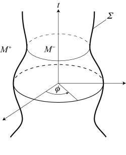
Figure 1: The world volume $\Sigma$ of the AT-shell divides the spacetime into two regions $M_{\pm}$.

The AT-shell divides the spacetime into two regions: one is the inside of the AT-shell $M^{-}$ and the other is the outside of it $M^{+}$ (see Fig. 1). By denoting the world volume of the AT-shell by $\Sigma$, the whole spacetime is given by $M=M^{-}\cup\Sigma\cup M^{+}$. Both regions $M^{\pm}$ have the whole cylinder symmetry, or in other words, the line element is written in the form,

$$ds^{2}=e^{2(\gamma-\psi)}(-dt^{2}+dr^{2})+\beta^{2}e^{-2\psi}d\phi^{2}+e^{2\psi}dz^{2},$$ (1)

where $\gamma$, $\psi$ and $\beta$ are functions that depend only on $t$ and $r$. We assume that both regions $M^{\pm}$ are vacuum. The domains of coordinates are $-\infty<t<\infty$, $-\infty<z<\infty$, $0\leq r<\infty$, and $0\leq\phi<2\pi$. The axis of rotational symmetry is located at $r=0$. The coordinate bases $\partial/\partial\phi$ and $\partial/\partial z$ are the rotational and translational Killing vectors, respectively.

The Einstein equations in the vacuum region lead to the equation for $\beta$, $\psi$ and $\gamma$ as

$$\beta^{\prime\prime}-\ddot{\beta}=0,$$ (2)

$$\beta(\ddot{\psi}-\psi^{\prime\prime})+\dot{\beta}\dot{\psi}-\beta^{\prime}\psi^{\prime}=0,$$ (3)

$$(\dot{\beta}^{2}-\beta^{\prime 2})\gamma^{\prime}+\beta\beta^{\prime}(\psi^{\prime 2}+\dot{\psi}^{2})-2\beta\dot{\beta}\dot{\psi}\psi^{\prime}+(\beta^{\prime}\beta^{\prime\prime}-\dot{\beta}\dot{\beta}^{\prime})=0$$ (4)

$$(\beta^{\prime 2}-\dot{\beta}^{2})\dot{\gamma}+\beta\dot{\beta}(\psi^{\prime 2}+\dot{\psi}^{2})-2\beta\beta^{\prime}\dot{\psi}\psi^{\prime}+(\dot{\beta}\beta^{\prime\prime}-\beta^{\prime}\dot{\beta}^{\prime})=0$$ (5)

$$\ddot{\gamma}-\gamma^{\prime\prime}+(\dot{\psi}^{2}-\psi^{\prime 2})=0,$$ (6)

where $\dot{A}$ and $A^{\prime}$ mean derivative of $A$ with respect to $t$ and $r$, respectively. In the original description of the AT shell, $\beta$ is set to be $r$, i.e., $\beta=r$. By contrast, we do not set it here so as to introduce the coordinate system comoving to the shell later.

The stress-energy tensor of the AT-shell is infinite since the finite energy is confined within the infinitesimally thin region. The Ricci tensor diverges on the AT-shell through the Einstein equations, and hence the AT shell is the so-called s.p. curvature singularity[11]. However, since the co-dimension of a shell is one, this singularity is so weak that the metric is defined on the AT-shell. Hence, even if the spacetime is singular on the AT-shell, it can consistently be treated by the Israel’s metric junction method [12, 13, 14]. The junction conditions between $M^{-}$ and $M^{+}$ at $\Sigma$ require the continuity of the metric and specify the discontinuity of the extrinsic curvature $K^{\pm}_{\alpha\beta}$ compatible with the stress-energy tensor of the AT-shell.

We require that the Killing vectors $\partial/\partial\phi$ and $\partial/\partial z$ are continuous at $\Sigma$, and this requirement leads to the continuities of the metric functions $\beta$ and $\psi$. We do not require the continuity of $\gamma$, and this means that the coordinate function $t$ and accordingly, the coordinate basis, $\partial/\partial t$, may not be continuous at the $\Sigma$. Although we can require that the coordinate function $t$ and accordingly, the coordinate basis, $\partial/\partial t$ is also continuous at $\Sigma$, we will not do so in this paper. This means that $\gamma$ may not be continuous at the AT-shell. The reason of this choice is that the solutions for the metric functions do not take simple forms in the continuous time coordinate, whereas the discontinuous one makes those solutions simple. The time coordinate for the interior region is denoted by $t_{-}$, whereas that for the exterior region is denoted by $t_{+}$. The radial coordinate at the AT-shell is denoted by $R(\tau)$, where $\tau$ is the proper time of an observer at rest on the shell.

We introduce the proper reference frame of an observer riding on the AT-shell as follows:

$${\bf e}_{(\tau)}=\frac{d}{d\tau}=X_{\pm}\frac{\partial}{\partial t_{\pm}}+V\frac{\partial}{\partial r}={\mbox{four velocity of the shell}},$$ (7)

$${\bf e}_{(n)}=\frac{d}{dn}=V\frac{\partial}{\partial t_{\pm}}+X_{\pm}\frac{\partial}{\partial r}={\mbox{outward unit vector normal to the shell}},$$ (8)

$${\bf e}_{(\phi)}=\frac{1}{\beta e^{-\psi}}\frac{\partial}{\partial\phi},$$ (9)

$${\bf e}_{(z)}=\frac{1}{e^{\psi}}\frac{\partial}{\partial z},$$ (10)

where

$$V:=\frac{dR}{d\tau},\quad\mbox{and}\quad X_{\pm}:=\frac{dt_{\pm}}{d\tau}=\sqrt{e^{-2(\gamma^{\pm}-\psi)}+V^{2}}.$$ (11)

The subscripts or superscripts $+$ and $-$ are used to denote quantities evaluated on the outer and inner faces of the shell, respectively.

Each constituent particle of the AT-shell has an identical rest mass. Half of the particles orbit around the symmetry axis in a right-handed direction with angular momentum per unit mass $\alpha$, and the other half orbit in the opposite, left-handed direction with angular momentum per unit rest mass $-\alpha$. Therefore, the net angular momentum of the AT-shell is zero. The absolute value of the specific linear momentum $u$ of a constituent particle, which is defined by

$$u:=\frac{\alpha}{\beta e^{-\psi}},$$ (12)

is an important quantity to describe the AT-shell. The other quantity characterizing the AT-shell is the shell’s rest mass per unit translational Killing length, which is denoted by $\lambda$. The rest mass of each constituent particle is conserved, so is $\lambda$. Then, the surface stress-energy tensor of the AT-shell is given by

$${\bf S}=\sigma{\bf e}_{(\tau)}\otimes{\bf e}_{(\tau)}+T{\bf e}_{(\phi)}\otimes{\bf e}_{(\phi)},$$ (13)

where we have defined the energy per unit area and the surface stress of the AT-shell as

$$\sigma:=\frac{\lambda\sqrt{1+u^{2}}}{2\pi\beta},\quad\mbox{and}\quad T:=\frac{\lambda u^{2}}{2\pi\beta\sqrt{1+u^{2}}},$$ (14)

respectively.

Israel has shown that the Einstein equations on the AT-shell reduce to

$$K^{+}_{\alpha\beta}-K^{-}_{\alpha\beta}=-8\pi\left(S_{\alpha\beta}-\frac{1}{2}S^{\mu}_{\mu}h_{\alpha\beta}\right),$$ (15)

where $K^{\pm}_{\alpha\beta}$ is the extrinsic curvature of the shell’s outer and inner face, and $h_{\alpha\beta}$ is the induced metric on the $\Sigma$.

Now, we impose the comoving condition for the AT-shell, i.e., $V=0$. The comoving condition fixes the metric function $\beta$, but it does not necessarily imply $\beta=r$. In this coordinate system, the coordinate radius $R$ at the AT-shell does not characterize the evolution of the shell, but its circumferential radius $\cal R$ defined by

$$\mathcal{R}:=\beta e^{-\psi}|_{r=R},$$ (16)

does instead of $R$.

In the comoving coordinate, the non-vanishing components of the extrinsic curvature are given by

$$K_{(\tau)(\tau)}=\psi_{,n}-\gamma_{,n},$$ (17)

$$K_{(\phi)(\phi)}=(\ln\beta)_{,n}-\psi_{,n},$$ (18)

$$K_{(z)(z)}=\psi_{,n}.$$ (19)

Therefore, the Israel’s junction conditions give the following equations:

$$\left[e^{-\gamma}e^{\psi}\left(\psi^{\prime}-\gamma^{\prime}\right)\right]^{+}_{-} = -\frac{2\lambda(1+2u^{2})}{\beta\sqrt{1+u^{2}}},$$ (20)

$$\left[e^{-\gamma}e^{\psi}\left(\frac{\beta^{\prime}}{\beta}-\psi^{\prime}\right)\right]^{+}_{-} = -\frac{2\lambda(1+2u^{2})}{\beta\sqrt{1+u^{2}}},$$ (21)

$$\left[e^{-\gamma}e^{\psi}\psi^{\prime}\right]^{+}_{-} = -\frac{2\lambda}{\beta\sqrt{1+u^{2}}},$$ (22)

where

$$\left[A\right]^{+}_{-}=A^{+}-A^{-}.$$ (23)

Using the continuity of $\psi$ and $\beta$ at $\Sigma$, we can rewrite the above equations as

$$\left[e^{-\gamma}\psi^{\prime}\right]^{+}_{-} = -\frac{2\lambda}{\beta\sqrt{1+u^{2}}}e^{-\psi},$$ (24)

$$\left[e^{-\gamma}\gamma^{\prime}\right]^{+}_{-} = \frac{4\lambda u^{2}}{\beta\sqrt{1+u^{2}}}e^{-\psi},$$ (25)

$$\left[e^{-\gamma}\beta^{\prime}\right]^{+}_{-} = -4\lambda\sqrt{1+u^{2}}e^{-\psi}.$$ (26)

These are the junction conditions under the comoving condition.

3 static solution

As was found by Apostolatos and Thorne[6], there is a static solution for the AT-shell which is regular except at the shell itself. In the interior region, the metric functions of the static solution are

$$\beta^{-}=r,\quad\psi^{-}=\psi_{s},\quad\gamma^{-}=0,$$ (27)

where $\psi_{s}$ is a constant. In the exterior region, the metric functions are

$$\beta^{+}=r,\quad\psi^{+}=\psi_{s}-2y\ln\frac{r}{R},\quad\gamma^{+}=2\ln(1+2y)+4y^{2}\ln\frac{r}{R},$$ (28)

where we have defined a parameter

$$y:=\frac{\alpha^{2}}{R^{2}e^{-2\psi_{s}}}.$$ (29)

The junction conditions require the relation

$$\lambda e^{-\psi_{s}}=\frac{y\sqrt{1+y}}{(1+2y)^{2}}.$$ (30)

Since we may set $\psi_{s}=0$ by rescaling the coordinates $t$, $r$ and $z$, the static solutions form a one parameter family. If we fix $y$, then the solution is uniquely determined, and hence $y$ is a good parameter to characterize the static solutions.

4 Perturbative analysis around the static solution

In this section, we give a perturbative analysis of the static AT-shell. If there is a smooth one-parameter family of dynamical exact solutions for the AT-shell, which includes a static solution as its member, we can construct dynamical solutions from the static solution by the perturbative method[15]. Here, we assume that such a one-parameter family exists. Denoting the parameter by $\varepsilon$, we write the metric functions in the form

$$\beta(t,r;\varepsilon)=\sum_{n=0}\varepsilon^{n}\beta_{n}(t,r),$$ (31)

$$\psi(t,r;\varepsilon)=\sum_{n=0}\varepsilon^{n}\psi_{n}(t,r),$$ (32)

$$\gamma(t,r;\varepsilon)=\sum_{n=0}\varepsilon^{n}\gamma_{n}(t,r).$$ (33)

The static solution is obtained by putting $\varepsilon=0$, or in other words, $\beta_{0}$, $\psi_{0}$ and $\gamma_{0}$ are functions given by (27) and (28) for the interior and exterior regions, respectively. We can derive the Einstein equations of each order with respect to $\varepsilon$, and solve them by successive approximation up to the order we need. In this paper, we solve the equations up to $O(\varepsilon)$, i.e., the linearized Einstein equations in the static background.

The Einstein equations of $O(\varepsilon)$ are

$$\beta_{1}^{\prime\prime}-\ddot{\beta}_{1}=0,$$ (34)

$$\beta_{0}\psi_{1}^{\prime\prime}+\beta_{0}^{\prime}\psi_{1}^{\prime}-\beta_{0}\ddot{\psi}_{1}+\beta_{1}\psi_{0}^{\prime\prime}+\beta_{1}^{\prime}\psi_{0}^{\prime}=0,$$ (35)

$$\gamma_{1}^{\prime\prime}-\ddot{\gamma}_{1}+2\psi_{0}^{{}^{\prime}}\psi_{1}^{\prime}=0,$$ (36)

$$\beta_{0}^{\prime}\beta_{1}^{\prime\prime}-2\beta_{0}^{{}^{\prime}}\gamma_{0}^{\prime}\beta_{1}^{\prime}+\beta_{0}\psi_{0}^{{}^{\prime}2}\beta_{1}^{\prime}+\beta_{0}^{\prime\prime}\beta_{1}^{\prime}+\beta_{0}^{\prime}\psi_{0}^{{}^{\prime}2}\beta_{1}-\beta_{0}^{{}^{\prime}2}\gamma_{1}^{\prime}+2\beta_{0}\beta_{0}^{\prime}\psi_{0}^{{}^{\prime}}\psi_{1}^{\prime}=0,$$ (37)

$$\beta_{0}^{\prime}\dot{\beta}_{1}^{\prime}-\beta_{0}\psi_{0}^{{}^{\prime}2}\dot{\beta}_{1}-\beta_{0}^{\prime\prime}\dot{\beta}_{1}-\beta_{0}^{{}^{\prime}2}\dot{\gamma}_{1}+2\beta_{0}\beta_{0}^{\prime}\psi_{0}^{\prime}\dot{\psi}_{1}=0.$$ (38)

Eqs. (34)–(36) are the evolution equations for $\beta_{1}$, $\psi_{1}$ and $\gamma_{1}$, whereas Eqs. (37) and (38) are the constraint equations which include no second order time derivative.

In order to study the stability of the static AT-shell, we assume that there is no energy input into the AT-shell. Therefore we impose the outgoing wave boundary condition in which there is no ingoing gravitational wave from past null infinity. In the interior region, we impose the regularity condition at the symmetric axis. Firstly, we solve these equations in the interior and exterior regions by imposing the regularity condition at the symmetry axis and the outgoing wave boundary condition, and then impose the junction conditions to glue these solutions at $\Sigma$.

4.1 Solutions for the interior region

By using the expression of the static solutions in the interior region (27), we rewrite the linearized Einstein equations for the interior region as

$$\beta_{1}^{-^{\prime\prime}}-\ddot{\beta}_{1}^{-}=0$$ (39)

$$\psi_{1}^{-^{\prime\prime}}+\frac{1}{r}\psi_{1}^{-^{\prime}}-\ddot{\psi}_{1}^{-}=0,$$ (40)

$$\gamma_{1}^{-^{\prime\prime}}-\ddot{\gamma}_{1}^{-}=0,$$ (41)

$$\beta_{1}^{-^{\prime\prime}}=\gamma_{1}^{-^{\prime}},$$ (42)

$$\dot{\beta}_{1}^{-^{\prime}}=\dot{\gamma}_{1}^{-}.$$ (43)

The last two equations can be integrated to give the relation

$$\beta_{1}^{-^{\prime}}+C^{-}=\gamma_{1}^{-},$$ (44)

where $C^{-}$ is an integration constant. Therefore, $\gamma_{1}^{-}$ is easily obtained once $\beta_{1}^{-}$ is known. The others are three homogeneous equations. Since the background solution is static, we can assume that all perturbations have a time dependence $e^{-i\omega_{-}t_{-}}$ and solve for $\omega_{-}$ in order to know whether complex or pure imaginary frequencies exist. The solutions for the three homogeneous equations are given by

$$\beta_{1}^{-}=\mbox{Re}\left[\ e^{-i\omega_{-}t_{-}}\left(A^{\beta^{-}}(\omega_{-})e^{i\omega_{-}r}+B^{\beta^{-}}(\omega_{-})e^{-i\omega_{-}r}\right)\right],$$ (45)

$$\psi_{1}^{-}=\mbox{Re}\left[e^{-i\omega_{-}t_{-}}\left(A^{\psi^{-}}(\omega_{-})H_{0}^{(1)}(\omega_{-}r)+B^{\psi^{-}}(\omega_{-})H_{0}^{(2)}(\omega_{-}r)\right)\right],$$ (46)

$$\gamma_{1}^{-}=\mbox{Re}\left[\ i\omega_{-}e^{-i\omega_{-}t_{-}}\left(A^{\beta^{-}}(\omega_{-})e^{i\omega_{-}r}-B^{\beta^{-}}(\omega_{-})e^{-i\omega_{-}r}\right)+C^{-}\right],$$ (47)

where $A^{\beta^{-}},B^{\beta^{-}},A^{\psi^{-}}$ and $B^{\beta^{-}}$ are functions of $\omega_{-}$. “Re”denotes the real part, and $H^{(1)}_{0}$, $H^{(2)}_{0}$ are the Hankel functions of the first and second kind of order $0$, respectively.

Now, we impose the regularity condition at the symmetric axis, $r=0$, in accordance with Hayward[16]. The regularity condition can be expressed in a geometrically invariant manner by using the norm of the Killing vectors,

$$\rho:=|\partial_{\phi}|=\beta e^{-\psi},\quad\ell:=|\partial_{z}|=e^{\psi}.$$ (48)

At the symmetric axis, $\rho$ should vanish. The axis is said to be regular if $\ell$ is finite and

$$\nabla\rho\cdot\nabla\rho=1+\mathcal{O}(\rho^{2}),$$ (49)

$$\nabla\rho\cdot\nabla\ell=\mathcal{O}(\rho),$$ (50)

$$\nabla\ell\cdot\nabla\ell=\mathcal{O}(1),$$ (51)

where $\nabla$ is the covariant derivative of the spacetime metric. These regularity conditions are satisfied if and only if

$$A^{\beta^{-}}+B^{\beta^{-}}=0,\quad A^{\psi^{-}}-B^{\psi^{-}}=0,\quad C^{-}=0.$$ (52)

Therefore, we obtain the regular interior solutions as

$$\beta_{1}^{-}=\mbox{Re}\left[e^{-i\omega_{-}t_{-}}A^{\beta^{-}}(\omega_{-})\left(e^{i\omega_{-}r}-e^{-i\omega_{-}r}\right)\right],$$ (53)

$$\psi_{1}^{-}=\mbox{Re}\left[2e^{-i\omega_{-}t_{-}}A^{\psi^{-}}(\omega_{-})J_{0}(\omega_{-}r)\right],$$ (54)

$$\gamma_{1}^{-}=\mbox{Re}\left[i\omega_{-}e^{-i\omega_{-}t_{-}}A^{\beta^{-}}(\omega_{-})\left(e^{i\omega_{-}r}+e^{-i\omega_{-}r}\right)\right],$$ (55)

where $J_{0}$ is the Bessel function of order $0$. If $\omega_{-}$ is real and negative, we have to replace $J_{0}(\omega_{-}r)$ by $J_{0}(|\omega_{-}|r)$. However, since we are interested in complex or pure imaginary solutions for $\omega_{-}$, we need not treat such a case.

4.2 Solutions for the exterior region

Using the fact that $\psi_{0}^{{}^{\prime}2}=-\gamma_{0}^{\prime\prime}$, the constraint equations (37) and (38) become

$$\beta_{1}^{+^{\prime\prime}}-(\gamma_{0}^{+^{\prime}}\beta_{1}^{+})^{\prime}+2\beta_{0}^{+}\psi_{0}^{+^{\prime}}\psi_{1}^{+^{\prime}}-\beta_{0}^{+^{\prime}}\gamma_{1}^{+^{\prime}}=0,$$ (56)

$$\dot{\beta}_{1}^{+^{\prime}}-\gamma_{0}^{+^{\prime}}\dot{\beta}_{1}^{+}+2\beta_{0}^{+}\psi_{0}^{+^{\prime}}\dot{\psi}_{1}^{+}-\beta_{0}^{+^{\prime}}\dot{\gamma}_{1}^{+}=0.$$ (57)

By noting that $\beta_{0}^{+}\psi_{0}^{+^{\prime}}$ is constant, we can integrate the above two equations and obtain

$$\gamma_{1}^{+}=\frac{1}{\beta_{0}^{+^{\prime}}}\left(\beta_{1}^{+^{\prime}}-\gamma_{0}^{+^{\prime}}\beta_{1}^{+}+2\beta_{0}^{+}\psi_{0}^{+^{\prime}}\psi_{1}^{+}\right)+C^{+},$$ (58)

where $C^{+}$ is an integration constant. By using the background solutions (28), the evolution equations for $\beta_{1}^{+},\psi_{1}^{+}$ and $\gamma_{1}^{+}$ become

$$\beta_{1}^{+^{\prime\prime}}-\ddot{\beta}_{1}^{+}=0,$$ (59)

$$\psi_{1}^{+^{\prime\prime}}+\frac{1}{r}\psi_{1}^{+^{\prime}}-\ddot{\psi}_{1}^{+}=-\frac{1}{r}(\psi_{0}^{+^{\prime}}\beta_{1}^{+})^{\prime},$$ (60)

$$\gamma_{1}^{+^{\prime\prime}}-\ddot{\gamma}_{1}^{+}+2\psi_{0}^{+^{\prime}}\psi_{1}^{+^{\prime}}=0.$$ (61)

Though the equation for $\psi_{1}^{+}$ is an inhomogeneous equation, one can easily see that $\psi_{0}^{+^{\prime}}\beta_{1}^{+}$ is a particular solution to the equation. By the same reason as the interior solutions, we can assume the time dependence $e^{-i\omega_{+}t_{+}}$ for the exterior solutions. The outgoing wave solutions for the above equations are written as

$$\beta_{1}^{+}=\mbox{Re}\left[A^{\beta^{+}}(\omega_{+})e^{-i\omega_{+}(t_{+}-r)}\right],$$ (62)

$$\psi_{1}^{+}=g_{\psi}^{+}-\frac{2y\beta_{1}^{+}}{r},$$ (63)

$$\gamma_{1}^{+}=\beta_{1}^{+^{\prime}}+\frac{4y^{2}}{r}\beta_{1}^{+}-4yg_{\psi}^{+}+C^{+},$$ (64)

where we have introduced the outgoing homogeneous solution for Eq. (60) as

$$g_{\psi}^{+}:=\mbox{Re}\left[A^{\psi^{+}}(\omega_{+})e^{-i\omega_{+}t_{+}}H_{0}^{(1)}(\omega_{+}r)\right].$$ (65)

If $\omega_{+}$ takes a negative real value, we have to replace $H_{0}^{(1)}(\omega_{+}r)$ by $H_{0}^{(2)}(|\omega_{+}|r)$ so as to keep the outgoing wave condition. However, since we are interested in complex or pure imaginary solutions for $\omega_{+}$, we need not treat such a case.

4.3 Solving the junction conditions at $\Sigma$

Now, we glue the interior solution to the exterior one at $\Sigma$. For that purpose, we have to relate the time coordinates $t_{-}$ and $t_{+}$ at $\Sigma$. Firstly, we relate $t_{-}$ and $t_{+}$ to $\tau$. From Eq.  (11) and the comoving condition $V=0$, we have

$$\frac{dt_{-}}{d\tau}=e^{-\gamma^{-}+\psi^{-}}=e^{\psi_{s}}+\varepsilon e^{\psi_{s}}(\psi_{1}^{-}-\gamma_{1}^{-})+{\cal O}(\varepsilon^{2}).$$ (66)

The second term in the right hand side in the above equation contributes in all relevant equations only of ${\cal O}(\varepsilon^{2})$, since the background solution does not depend on $t_{-}$. Therefore, we may set, in the linearized equations, $t_{-}=e^{\psi_{s}}\tau$. Similarly, for the exterior time coordinate, we may set $t_{+}=(1+2y)^{-2}e^{\psi_{s}}\tau$. From these relations, we obtain

$$t_{+}=(1+2y)^{-2}t_{-}~{}~{}~{}{\rm on}~{}~{}\Sigma.$$ (67)

The continuity of $\beta$ and $\psi$ at $\Sigma$ gives

$$\beta_{1}^{-}|_{r=R}=\beta_{1}^{+}|_{r=R},$$ (68)

$$\psi_{1}^{-}|_{r=R}=\psi_{1}^{+}|_{r=R}.$$ (69)

The above conditions imply that the time dependences of solutions for $\beta_{1}$ and $\psi_{1}$ in $M_{\pm}$ are the same at $\Sigma$, and hence $\omega_{+}t_{+}=\omega_{-}t_{-}$ should be satisfied. Then from Eq. (67), we have $\omega_{+}=(1+2y)^{2}\omega_{-}$. Hereafter, for notational simplicity, we abbreviate $\omega_{-}$ as $\omega$, or equivalently,

$$\omega_{-} = \omega,$$ (70)

$$\omega_{+} = (1+2y)^{2}\omega.$$ (71)

The junction conditions of $O(\varepsilon)$ are obtained by directly expanding Eqs. (24), (25) and (26) with respect to $\varepsilon$ as

$$\left[e^{-\gamma_{0}}(\psi_{1}^{\prime}-\gamma_{1}\psi_{0}^{\prime})\right]^{+}_{-}=\frac{2y}{R(1+2y)^{2}}\left(\frac{1}{1+y}\frac{\beta_{1}^{-}}{R}+\frac{1+2y}{1+y}\psi_{1}^{-}\right)\biggr{|}_{r=R},$$ (72)

$$\left[e^{-\gamma_{0}}(\gamma_{1}^{\prime}-\gamma_{1}\gamma_{0}^{\prime})\right]^{+}_{-}=\frac{4y^{2}}{R(1+2y)^{2}}\left(\frac{1}{1+y}\psi_{1}^{-}-\frac{3+2y}{1+y}\frac{\beta_{1}^{-}}{R}\right)\biggr{|}_{r=R},$$ (73)

$$\left[e^{-\gamma_{0}}\left(\beta_{1}^{\prime}-\gamma_{1}\beta_{0}^{\prime}\right)\right]^{+}_{-}=\frac{4y(1+y)}{(1+2y)^{2}}\left(\frac{1}{1+y}\psi_{1}^{-}+\frac{y}{1+y}\frac{\beta_{1}^{-}}{R}\right)\biggr{|}_{r=R}.$$ (74)

Since $\beta_{1}$ and $\psi_{1}$ are continuous at $r=R$, one may replace $\beta_{1}^{-}$ and $\psi_{1}^{-}$ in the right hand side of the above equations with $\beta_{1}^{+}$ and $\psi_{1}^{+}$, respectively. By substituting Eq. (44) with $C^{-}=0$ and Eq. (58) into Eq. (74), and by using the static solutions (27) and (28), we obtain

$$C^{+}=0.$$ (75)

Then, four equations (68), (69), (72) and (73) determine four amplitudes $A^{\beta^{\pm}}$ and $A^{\psi^{\pm}}$.

The continuity conditions (68) and (69) give

$$(1+2y)^{2}e^{i\omega\hat{R}}\frac{A^{\beta^{+}}}{R}-2i\frac{A^{\beta^{-}}}{R}\sin\omega R=0,$$ (76)

$$(1+2y)^{2}A^{\psi^{+}}H_{0}^{(1)}(\omega\hat{R})-{2y}(1+2y)^{2}e^{i\omega\hat{R}}\frac{A^{\beta^{+}}}{R}-2A^{\psi^{-}}J_{0}(\omega R)=0,$$ (77)

where, for notational simplicity, we have introduced a new quantity $\hat{R}=(1+2y)^{2}R$. The junction conditions (72) and (73) lead

$$-\omega R(1+2y)^{4}A^{\psi^{+}}H_{1}^{(1)}(\omega\hat{R})-{8y^{2}}(1+2y)^{2}A^{\psi^{+}}H_{0}^{(1)}(\omega\hat{R})+2(1+2y)^{2}\omega RA^{\psi^{-}}J_{1}(\omega R)$$

$$+{2y}(1+4y^{2})(1+2y)^{2}e^{i\omega\hat{R}}\frac{A^{\beta^{+}}}{R}-\frac{4iy}{(1+y)}\frac{A^{\beta^{-}}}{R}\sin\omega R-\frac{4y(1+2y)}{(1+y)}A^{\psi^{-}}J_{0}(\omega R)=0,$$

(78)

and

$$-\omega^{2}R^{2}(1+2y)^{6}e^{i\omega\hat{R}}\frac{A^{\beta^{+}}}{R}-{4y^{2}(1+4y^{2})}(1+2y)^{2}e^{i\omega\hat{R}}\frac{A^{\beta^{+}}}{R}+4y(1+2y)^{4}\omega RA^{\psi^{+}}H_{1}^{(1)}(\omega\hat{R})$$

$$+{16y^{3}}(1+2y)^{2}A^{\psi^{+}}H_{0}^{(1)}(\omega\hat{R})+2i(1+2y)^{2}\omega^{2}R^{2}\frac{A^{\beta^{-}}}{R}\sin\omega R-\frac{8y^{2}}{(1+y)}A^{\psi^{-}}J_{0}(\omega R)$$

$$+\frac{8iy^{2}(3+2y)}{(1+y)}\frac{A^{\beta^{-}}}{R}\sin\omega R=0,$$ (79)

respectively. These equations can be put into the following matrix form:

$$\sum_{j=1}^{4}M_{ij}A^{j}=0,$$ (80)

where $i=1,2,3,4$ and we have defined

$$A^{1}:=A^{\psi^{+}},\quad A^{2}:=\frac{A^{\beta^{+}}}{R},\quad A^{3}:=A^{\psi^{-}},\quad A^{4}:=\frac{A^{\beta^{-}}}{R}.$$ (81)

The components of the matrix $M_{ij}$ are given by

$$M_{11}=M_{13}=M_{24}=0,$$ (82)

$$M_{12}=(1+2y)^{2}e^{i\omega\hat{R}},$$ (83)

$$M_{14}=-2i\sin\omega R,$$ (84)

$$M_{21}=(1+2y)^{2}H_{0}^{(1)}(\omega\hat{R}),$$ (85)

$$M_{22}=-{2y}(1+2y)^{2}e^{i\omega\hat{R}},$$ (86)

$$M_{23}=-2J_{0}(\omega R),$$ (87)

$$M_{31}=-\omega R(1+2y)^{4}H_{1}^{(1)}(\omega\hat{R})-{8y^{2}}(1+2y)^{2}H_{0}^{(1)}(\omega\hat{R}),$$ (88)

$$M_{32}=2y(1+4y^{2})(1+2y)^{2}e^{i\omega\hat{R}},$$ (89)

$$M_{33}=2(1+2y)^{2}\omega RJ_{1}(\omega R)-\frac{4y(1+2y)}{(1+y)}J_{0}(\omega R),$$ (90)

$$M_{34}=-\frac{4iy}{(1+y)}\sin\omega R,$$ (91)

$$M_{41}=4y(1+2y)^{4}\omega RH_{1}^{(1)}(\omega\hat{R})+{16y^{3}}(1+2y)^{2}H_{0}^{(1)}(\omega\hat{R}),$$ (92)

$$M_{42}=-\omega^{2}R^{2}(1+2y)^{6}e^{i\omega\hat{R}}-{4y^{2}(1+4y^{2})}(1+2y)^{2}e^{i\omega\hat{R}},$$ (93)

$$M_{43}=-\frac{8y^{2}}{(1+y)}J_{0}(\omega R),$$ (94)

$$M_{44}=2i(1+2y)^{2}\omega^{2}R^{2}\sin\omega R+\frac{8iy^{2}(3+2y)}{(1+y)}\sin\omega R.$$ (95)

In order that there are non-trivial solutions for Eq. (80), the following equation should be satisfied;

$$\mbox{det}\left(M_{ij}\right)=0.$$ (96)

For fixed $y$ and $R$, this is an equation for frequency $\omega$. Here, instead of (96), we consider a real equation

$$|\mbox{det}\left(M_{ij}\right)|^{2}=0.$$ (97)

Using a dimensionless quantity $z=\omega R$, Eq. (97) is rewritten in the form

$$\frac{256y^{2}(1+2y)^{12}}{(1+y)^{2}}F(z)\sin^{2}z=0,$$ (98)

where $F(z)$ is defined by

$$F(z) := \Bigg{[}\bigg{(}2y(1+y)\left((1+6y+4y^{2})z^{2}-2y\right)J_{0}(z)$$

$$\qquad+z\left(y(2+y(1+2y)^{2})-(1+y)^{2}(1+2y)^{2}z^{2}\right)J_{1}(z)\bigg{)}H_{0}^{(1)}\big{(}(1+2y)^{2}z\big{)}$$

$$\qquad+(1+2y)^{2}z\bigg{(}(z^{2}+y(2+y)(z^{2}-1))J_{0}(z)+2y(1+y)zJ_{1}(z)\bigg{)}H_{1}^{(1)}\big{(}(1+2y)^{2}z\big{)}\Bigg{]}$$

$$\Bigg{[}\bigg{(}2y(1+y)\left((1+6y+4y^{2})z^{2}-2y\right)J_{0}(z)$$

$$\qquad+z\left(y(2+y(1+2y)^{2})-(1+y)^{2}(1+2y)^{2}z^{2}\right)J_{1}(z)\bigg{)}H_{0}^{(2)}\big{(}(1+2y)^{2}z\big{)}$$

$$+(1+2y)^{2}z\bigg{(}(z^{2}+y(2+y)(z^{2}-1)J_{0}(z)+2y(1+y)zJ_{1}(z))\bigg{)}H_{1}^{(2)}\big{(}(1+2y)^{2}z\big{)}\Bigg{]}.$$

It is easily seen that, for integer $n$, there are infinitely large numbers of real solutions $z=n\pi$, or equivalently,

$$\omega=\frac{n\pi}{R}.$$ (100)

These are radial oscillation modes of the shell around the static configuration. The existence of these oscillation modes is compatible with the C-energy argument given by Apostolatos and Thorne[6]. The gravitational emission may cause the damping of the oscillation, but this effect appears in ${\cal O}(\varepsilon^{2})$.

4.4 Unstable modes

In this subsection, we look for zero points of the function $F(z)$ in complex $z$ plane. We solve the equation

$$F(z)=0,$$ (101)

by using “FindRoot”program in Mathematica (version 7.0). As mentioned, the parameter $y$ characterizes the static solution, and hence we search for the solutions of $\omega$ as a function of $y$.

Since we invoked the numerical method to find the solutions, we have investigated a limited number of points in the domain $0\leq y<\infty$, not all $y$. But, as far as we have investigated, there exists at least one unstable mode for each $y$. Therefore, it is reasonable to conclude that there are unstable modes for all $y\geq 0$. The angular frequency $\omega$ of the unstable solution is written in the form

$$\omega=\omega_{\rm R}(y)+i\omega_{\rm I}(y),$$ (102)

where $\omega_{\rm R}$ is a real function of $y$, and $\omega_{\rm I}$ is also a real function of $y$ but is positive. We also found that if $\omega=\omega_{\rm R}+i\omega_{\rm I}$ is a solution, then $\omega=\omega_{\rm R}-i\omega_{\rm I}$ is also a solution.

We have found sixth classes of the unstable solutions. We depict $\omega_{\rm R}$ and $\omega_{\rm I}$ of the first class as functions of $y$ in Fig. 2, whereas those of the second, third, fourth, fifth and sixth classes are dipicted in Figs. 3–7, respectively.

Figure 2: The solutions of the first class are depicted. For $y\gtrsim 4.61$, the complex modes in this class become pure imaginary.

Figure 3: The solutions of the second class are depicted. For $y\gtrsim 1.4$, the complex modes in this class become pure imaginary.

In the case of the first class, the real part $\omega_{\rm R}$ increases from zero for $0\leq y\lesssim 0.6$, decreases for $0.6\lesssim y\lesssim 4.61$ and then becomes very tiny value $\epsilon$ for $y\gtrsim 4.61$. The maximum value of $\omega_{\rm R}$ is about $0.579R^{-1}$ at $y=0.6$. The tiny value $\epsilon$ depends on initial values in numerical investigation, and therefore $\epsilon$ will be a numerical error. Hence, it is reasonable to conclude that the numerical solutions with the form of $\omega=\epsilon\pm i\omega_{I}$ correspond to pure imaginary solutions. The imaginary part $\omega_{\rm I}$ of the first class increases from zero for $0\leq y\lesssim 4.61$ and bifurcates at $y\simeq 4.61$: one sequence monotonically increases and the other monotonically decreases for $4.61\lesssim y$. At $y\simeq 4.61$, the derivatives of both $\omega_{\rm R}$ and $\omega_{\rm I}$ with respect to $y$ are discontinuous.

In the case of the second class, the real part $\omega_{\rm R}$ increases for $y\lesssim 1.4$ and becomes very tiny value for $y\gtrsim 1.4$. By the same reason as in the first class, it is reasonable to conclude that these solutions are pure imaginary. The imaginary part $\omega_{\rm I}$ decreases for $y\lesssim 0.8$ and increases from 0.89$R^{-1}$ for $0.8\lesssim y$, approaching $R^{-1}$ as $y\rightarrow\infty$. The imaginary part $\omega_{\rm I}$ of the second class is larger than that of the first class.

Figure 4: The solutions of the third class are depicted.

In the case of the third class, the real part $\omega_{\rm R}$ monotonically increases and approaches 0 as $y$ increases. The imaginary part $\omega_{\rm I}$ decreases for $y\lesssim 0.4$ and increases from 0.169$R^{-1}$ to 0.236$R^{-1}$ for $0.4\lesssim y\lesssim 0.7$. For $0.7\lesssim y$, $\omega_{\rm I}$ decreases and approaches 0 as $y$ increases.

Figure 5: The solutions of the fourth class are depicted.

Figure 6: The solutions of the fifth class are depicted. At $y\simeq 4.62$, the solution in this class becomes pure imaginary and this class seems to connect to the pure imaginary modes in the first class.

Figure 7: The solutions of the sixth class are depicted.

In the case of fourth class, the real part $\omega_{\rm R}$ monotonically increases. The imaginary part $\omega_{\rm I}$ monotonically decreases and approaches 0.

The fifth class has monotonically increasing $\omega_{\rm R}$ for $y\lesssim 4.61$. At $y\simeq 4.62$, $\omega_{\rm R}$ becomes very tiny value, and for $y\gtrsim 4.62$ the solution becomes pure imaginary. The imaginary part $\omega_{\rm I}$ monotonically decreases to 0.075$R^{-1}$ for $y\lesssim 0.8$ and monotonically increases for $0.8\lesssim y\lesssim 4.61$. At $y=4.62$, the solution coincides with that of the first class. Therefore, this class seems to connect to the pure imaginary modes in the first class for $y\gtrsim 4.62$.

In the case of sixth class, the real part $\omega_{\rm R}$ monotonically increases and approaches 0. The imaginary part $\omega_{\rm I}$ monotonically decreases to 0.016$R^{-1}$ for $y\lesssim 0.44$ and increases to 0.24$R^{-1}$ for $0.44\lesssim y\lesssim 0.64$. For $0.64\lesssim y$, $\omega_{\rm I}$ decreases and approaches 0.

In order to understand what the existence of the unstable modes implies, we investigate the circumferential radius ${\cal R}$ of the shell. The perturbation of $O(\varepsilon)$ for the circumference radius of the AT shell is

$${\cal R}_{1} = (\beta_{1}e^{-\psi_{0}}-\beta_{0}\psi_{1})|_{r=R}$$ (103)

$$= \mbox{Re}\biggl{[}e^{-i\omega t_{-}}\Bigl{[}(e^{-\psi_{s}}+y)e^{i\omega\hat{R}}A^{\beta^{+}}(\omega)-RH_{0}^{(1)}(\omega\hat{R})A^{\psi^{+}}(\omega)\Bigr{]}\biggr{]}.$$

From the above equation, we can see that ${\cal R}_{1}$ is written symbolically in the form

$${\cal R}_{1}=\mbox{Re}\left[e^{-i\omega t_{-}}\left(C_{1}+iC_{2}\right)\right] = \sqrt{C_{1}^{2}+C_{2}^{2}}~{}e^{\omega_{I}t_{-}}\cos(\omega_{R}t_{-}-\phi),$$ (104)

where $C_{1}$ and $C_{2}$ are real numbers, and we have introduced a constant $\phi:=\tan^{-1}C_{2}/C_{1}$. The above equation implies that, if $\omega_{\rm R}$ does not vanish, the circumference radius oscillates and its amplitude grows exponentially with time. If $\omega_{\rm R}$ vanishes, there is a mode of which the shell does not oscillate radially but just expands or contracts exponentially. In both cases, the static shell is unstable up to the linear order.

When $\omega_{R}=0$, whether the AT-shell expands or contracts is determined by initial condition. In this case, ${\cal R}_{1}$ can be expressed as

$${\cal R}_{1}=e^{\omega_{I}t_{-}}C_{1}.$$ (105)

Therefore, if ${\cal R}_{1}$ is initially positive, then $C_{1}$ is positive and we find that the AT-shell expands exponentially. By contrast, if ${\cal R}_{1}$ is initially negative, then $C_{1}$ is negative and it contracts exponentially. This behavior of the AT-shell can be understood as infinite period limit ($T=2\pi/\omega_{R}\to\infty$) of the oscillation behavior (104).

The appearance of the pure imaginary modes depends on the parameter $y$. By using the speed of orbital motion of each constituent particle measured by an observer who rides on the static AT shell, say $v$, the parameter $y$ can be expressed as[6]

$$y=\frac{v^{2}}{1-v^{2}}.$$ (106)

It is easy to see that $y$ is a monotonically increasing function of $v$. If the velocity $v$ of each constituent particle is smaller than a critical value $v_{\rm c}\simeq 0.76$ which corresponds to $y\simeq 1.4$, the amplitude of the radial oscillation grows, whereas if $v>v_{\rm c}$, circumferential radius will expands or contracts exponentially with time.

5 summary and discussion

We have investigated linear perturbation of the AT-shell around the static solution, and have found that the static state is unstable in the sense that, if the speed of orbital motion of the constituent particles (denoted by $v$) is small, the perturbation of the shell’s circumference radius oscillates with exponentially growing amplitude and the shell does not settle down into the static configuration, and if $v$ is larger than the critical value $v_{\rm c}\simeq 0.76$, the shell just expands or contracts exponentially with time. Whether the shell expands or contracts for large velocity depends on the initial condition. If initially the circumference radius is larger than that of the static shell, then the AT-shell just expands exponentially. By contrast, if initially it is smaller than that of the static shell, the AT-shell just contracts exponentially.

Since we invoked the numerical method to find the solutions, we have investigated a limited number of points in the domain $0\leq y<\infty$, not all $y$. But, as far as we have investigated, there exists at least one unstable mode for each $y$. Therefore, it is reasonable to conclude that the static AT-shell is unstable for all $y$ up to $O(\varepsilon)$.

This result is compatible with the previous work given in Ref. [References] which showed that there exist momentarily static and radiation free initial states of the AT-shell which do not settle down into the static state, unless gravitational radiation extracts an infinite amount of C-energy from the AT-shell. More concretely, in this study, it was shown that, if the initial circumference radius of the AT-shell is greater than that of the expected final static state (having fixed $\alpha,\lambda,R$ and $\psi_{s}$), then the AT-shell cannot settle down into the static state, and if the initial circumference radius of the AT-shell is smaller than that of the static state, then it is not forbidden that the AT-shell settles down into the equilibrium static configuration. However, the existence of the unstable modes in our perturbation analysis does not depend on whether the initial circumference radius is greater than that of the static state or not. It means that, even if the initial circumference is smaller than that of the expected static shell, the AT-shell does not settle down into the static state.

Hamity, C$\acute{\mbox{e}}$cere and Barraco[10] discussed the stability of the AT-shell and concluded that for $y<0.78049$ ($\sqrt{y}<0.8836$), the static configuration is stable and for $y>0.78049$ ($\sqrt{y}>0.8836$), it is unstable. Their result seems to be inconsistent to Ref.[References], and further, in the present analysis, we do not find any evidence for it. They investigated only the sequence of the static configuration by a Gedanken experiment. However, it should be noted that in order to obtain a definite conclusion on the stability of the static AT-shell, it would be necessary to solve the Einstein equations. In contrast to Hamity et al., we have solved the Einstein equations, although we have used linear approximation.

Our perturbation analysis shows that the static AT-shell solution is unstable but does not say anything about the shell’s finial state. To make it clear, perturbation theory will not be adequate and we will have to solve full equations by using numerical relativity. These will be future works.

References

- [1] A. Einstein and N. Rosen, J. Franklin Inst. 223, 43 (1937).
- [2] G. Beck, Z. Physik 33, 713 (1925).
- [3] L. Marder, Proc. Roy. Soc. (London) A244, 524 (1958).
- [4] J. J. Stachel, J. Math. Phys 7, 1321 (1966).
- [5] T. Piran, Phys. Rev. Lett. 41, 1085 (1978).
- [6] T. A. Apostolatos and K. S. Thorne, Phys. Rev. D 46 2435 (1992).
- [7] The C-energy has been proposed by Thorne in the paper K. S. Thorne, Phys. Rev. 138, B251 (1965). It is a quasilocal energy included within a cylinder per unit Killing length.
- [8] K. -i. Nakao, D. Ida, Y. Kurita, Phys. Rev. D77, 044021 (2008). [arXiv:0711.0243 [gr-qc]].
- [9] R. J. Gleiser, M. A. Ramirez, [arXiv:1106.3122 [gr-qc]].
- [10] V. H. Hamity, M. A. Ccere, D. E. Barraco, Gen. Rel. Grav. 41, 2657-2676 (2009). [arXiv:0709.1933 [gr-qc]].
- [11] S. W. Hawking and G. F. R. Ellis, Large Scale Structure of Space-time , p. 260 (Cambridge University Press, Cambridge, 1973).
- [12] W. Israel, Nuovo. Cimento 44B, 1 (1966)
- [13] W. Israel, Nuovo. Cimento 48B, 463 (1967)
- [14] W. Israel, Phys. Rev. 153, 1388 (1967)
- [15] R. M. Wald, General Relativity, Section 7.5 (The University of Chicago Press, Chicago and London, 1984).
- [16] S. A. Hayward, Class. Quant. Grav. 17, 1749-1764 (2000).