Lie group analysis for multi-scale plasma dynamics

Abstract

An application of approximate transformation groups to study dynamics of a system with distinct time scales is discussed. The utilization of the Krylov-Bogoliubov-Mitropolsky method of averaging to find solutions of the Lie equations is considered. Physical illustrations from the plasma kinetic theory demonstrate the potentialities of the suggested approach. Several examples of invariant solutions for the system of the Vlasov-Maxwell equations for the two-component (electron-ion) plasma are presented.

1 Introduction

In analyzing various physical systems we frequently deal with a situation when a complicated dynamics of different systems appears as a superposition of “fast” and “slow” motions with incommensurable characteristic scales, for example, slow evolution of “background” system characteristics accompanied by fast oscillations in the vicinity of a background state. This type of behavior seems typical for various linear and nonlinear problems (numerous examples are found in [1, 2]), e.g. for celestial mechanics in studies of a motion of planets, for mechanics when treating oscillatory regimes of systems with slowly varying parameters, for various nonlinear problems of multi-component plasma.

The availability of different scales (though the origin of these scales depends upon the particular system of interest) allows to simplify the analysis of the complicated dynamics by treating “fast” and “slow” motions separately. These ideas underlie an essence of asymptotic analytical approaches, the method of averaging [4, 3], the method of multiple scales [1], and other asymptotic methods (see, e.g., [1, 2]).

As to relation of modern group analysis to nonlinear dynamics here we will point to an interpenetration of ideas from both fields: on one hand the use of the Lie group theory in asymptotic methods for integration of nonlinear differential equations gives (in combination with the Hausdorff formula) the theoretical basis for the method of averaging [3] and provides a regular procedure for calculating the asymptotic series in this method [5, 2, 6]. On the other hand an introduction of multiple-scales approach to modern group analysis [7] enhances the potentiality of approximate transformation groups [8].

The present paper uses the Krylov-Bogoliubov-Mitropolsky method (KBM-method) of averaging in group analysis of the system of equations that describes the evolution of plasma particles in multi-component plasma. The linearity of the group determining equations plays the decisive role in separating fast and slow terms in coordinates of a group generator and in successive use of the KBM-method for constructing the asymptotic solutions of the Lie group equations.

The paper is organized as follows: in Section 2 we introduce the basic equations for evolution of a two component plasma and introduce small parameters which give rise to different time and spatial scales for distinct plasma components. In the next Section 3 we describe the solution of determining equations, which define approximate Lie point symmetry group. The use of KBM-method in finding solutions of the Lie group equations constitutes the basis of the Section 4. Several examples of an application of the suggested approach are presented in Section 5 and Section 6. In the Conclusion we discuss the results obtained and the future application of the KBM-method in modern group analysis.

2 Basic Equations: Electron-ion Plasma

We start with kinetic equations for distribution functions, $f^{e}$ and $f^{i}$,

$$\partial_{t}f^{e}+v^{e}\partial_{x}f^{e}-(e/m)E\partial_{v^{e}}f^{e}=0\,,\quad\partial_{t}f^{i}+v^{i}\partial_{x}f^{i}+(Ze/M)E\partial_{v^{i}}f^{i}=0\,,$$ (1)

for both species of two-component plasma consisting of electrons and ions with mass $m$ and $M$ and charges $e^{e}=-e$ and $e^{i}=Ze$, where $Z$ is a charge number, and equations for a self-consistent electric field $E$

$$\partial_{x}E=4\pi\rho\,,\quad\partial_{t}E=-4\pi j\,,\quad\partial_{t}\rho+\partial_{x}j=0\,.$$ (2)

Here charge $\rho$ and current $j$ densities are related to moments of the distribution functions via nonlocal material relations:

$$\rho=e\left[Z\int\textrm{d}v^{i}f^{i}-\int\textrm{d}v^{e}f^{e}\right]\,,\quad j=e\left[Z\int\textrm{d}v^{i}v^{i}f^{i}-\int\textrm{d}v^{e}v^{e}f^{e}\right]\,.$$ (3)

Equations (1)-(3) are known as a system of the Vlasov-Maxwell equations for a collisionless plasma. We are interested in the solution of the Cauchy problem for kinetic equations (1) with the initial conditions

$$f^{e}|_{t=0}=f^{e}_{0}(x,v^{e})\,,\quad f^{i}|_{t=0}=f^{i}_{0}(x,v^{i})\,,$$ (4)

which depend on a particular physical problem. In what follows we consider an evolution of localized plasma bunches and assume sufficiently smooth (e.g., Maxwellian) initial distribution functions with electron $T_{e}$ and ion $T_{i}$ temperatures and initial densities of electrons $n^{e}(x)=\int\textrm{d}v^{e}f^{e}_{0}$ and ions $n^{i}(x)=\int\textrm{d}v^{i}f^{i}_{0}$ with the characteristic scale $L$. Below we consider a typical situation when $L$ is much greater than the Debye radius of electrons $r_{De}=\sqrt{T_{e}/(4\pi n^{e}_{0}e^{2})}$. The difference in mass of plasma particles specifies two different time scales, namely dimensionless time $\omega_{Le}t$ for “fast” electron motions and $\tau=\mu t$ for “slow” motions, $\mu=\sqrt{Zm/M}\ll 1$. It is natural that electrons are involved in both fast and slow motions, hence the electron distribution function depends on both $t$ and $\tau$. On the contrary, we consider ions not involved in fast motions. It means that the ion distribution function does not depend upon fast time $t$, but only upon slow time $\tau$. It also means that averaging upon fast time eliminates the fast component $\tilde{E}$ of the electric field $E={\tilde{E}}+{\bar{E}}$ in the ion kinetic equation that contains only the slow electric field $\bar{E}$. Then introducing dimensionless variables, electron velocity $u=v^{e}/V_{Te}$, $V_{Te}=\sqrt{T_{e}/m}$, dimensionless ion velocity $w=v^{i}/c_{s}$, $c_{s}=\sqrt{ZT_{e}/M}$, dimensionless electric field $p=\varepsilon(eEL/T_{e})$ , $\varepsilon=r_{De}/L\ll 1$ and dimensionless distribution functions $f^{e}=(n^{e}_{0}/V_{Te})g$, $f^{i}=(n^{e}_{0}/(Zc_{s}))f$, $n^{e(i)}_{0}=n^{e(i)}(0)$ we come to the following system of basic equations in dimensionless variables

$$\partial_{t}g+\mu\partial_{\tau}g+\varepsilon u\partial_{x}g-p\partial_{u}g=0\,,\quad\partial_{\tau}f+\varepsilon w\partial_{x}f+\bar{p}\partial_{w}f=0\,,$$ (5)

$$\varepsilon\partial_{x}p=\int\textrm{d}wf-\int\textrm{d}ug\,,\quad\partial_{t}p+\mu\partial_{\tau}p=-\mu\int\textrm{d}wwf+\int\textrm{d}uug\,.$$ (6)

From the group analysis point of view this system of equations should be supplemented by the four additional equalities,

$$\partial_{w}g=0\,,\quad\partial_{u}f=0\,,\quad\partial_{u}p=0\,,\quad\partial_{w}p=0\,,$$ (7)

which are evident from the physical point of view.

3 Lie symmetry group

The Lie point symmetry group admitted by the system (5) and (6) is defined by a symmetry group generator

$$X=\xi^{1}\partial_{t}+\xi^{2}\partial_{x}+\xi^{3}\partial_{u}+\xi^{4}\partial_{w}+\xi^{5}\partial_{\tau}+\eta^{1}\partial_{g}+\eta^{2}\partial_{p}+\eta^{3}\partial_{f}\,.$$ (8)

In the canonical form this generator is written as

$$Y=\kappa^{1}\partial_{g}+\kappa^{2}\partial_{p}+\kappa^{3}\partial_{f}\,,$$ (9)

$${\kappa}^{1}={\eta}^{1}-{\xi}^{1}\partial_{t}g-{\xi}^{2}\partial_{x}g-{\xi}^{3}\partial_{u}g-{\xi}^{5}\partial_{\tau}g\,,$$

$${\kappa}^{2}={\eta}^{2}-{\xi}^{1}\partial_{t}p-{\xi}^{2}\partial_{x}p-{\xi}^{5}\partial_{\tau}p\,,$$

$${\kappa}^{3}={\eta}^{3}-{\xi}^{2}\partial_{x}f-{\xi}^{4}\partial_{w}f-{\xi}^{5}\partial_{\tau}f\,.$$

When applying group generator (9) to (5), (6) and (7) we get a system of determining equations for coordinates $\xi^{i}$, $\eta^{i}$ of the generator (8),

$$D_{t}{\kappa}^{1}+\mu D_{\tau}{\kappa}^{1}+\varepsilon uD_{x}{\kappa}^{1}-pD_{u}{\kappa}^{1}-{\kappa}^{2}\partial_{u}g=0\,,$$ (10)

$$D_{\tau}{\kappa}^{3}+\varepsilon wD_{x}{\kappa}^{3}+\bar{p}D_{w}{\kappa}^{3}-{\bar{\kappa}}^{2}\partial_{w}f=0\,,$$

$$D_{w}{\kappa}^{1}=0\,,\quad D_{u}{\kappa}^{3}=0\,,\quad D_{u}{\kappa}^{2}=0\,,\quad D_{w}{\kappa}^{2}=0\,,$$

$$\varepsilon D_{x}{\kappa}^{2}-\int\textrm{d}w{\kappa}^{3}+\int\textrm{d}u{\kappa}^{1}=0\,,$$ (11)

$$D_{t}{\kappa}^{2}+\mu D_{\tau}{\kappa}^{2}+\mu\int\textrm{d}ww{\kappa}^{3}-\int\textrm{d}uu{\kappa}^{1}=0\,,$$

which should be solved in view of the basic equations (5), (6), (7) and all their differential consequences. Here $D_{t}$, $D_{\tau}$, $D_{x}$, $D_{u}$ and $D_{w}$ are total differentiations with respect to the variable denoted by lower index,

$$D_{t}=\partial_{t}+(\partial_{t}g)\,\partial_{g}+(\partial_{t}p)\,\partial_{p}\,,$$ (12)

$$D_{\tau}=\partial_{\tau}+(\partial_{\tau}g)\,\partial_{g}+(\partial_{\tau}f)\,\partial_{f}+(\partial_{\tau}p)\,\partial_{p}\,,$$

$$D_{x}=\partial_{x}+(\partial_{x}g)\,\partial_{g}+(\partial_{x}f)\,\partial_{f}+(\partial_{x}p)\,\partial_{p}\,,$$

$$D_{u}=\partial_{u}+(\partial_{u}g)\,\partial_{g}\,,\quad D_{w}=\partial_{w}+(\partial_{w}f)\,\partial_{f}\,.$$

To find coordinates $\xi^{i}$, $\eta^{i}$ from the system of determining equations we use the approach developed in [9] (see also [15, Chapter 4]). Following this technique we separate the determining equations for $\xi^{i}$ and $\eta^{i}$ into local determining equations, (10), which arise from invariance of (5), (7), and nonlocal determining equations, (11), which follow from invariance conditions for (6). Solutions of local determining equations give the so-called intermediate symmetry [9].

Two distinct moments should be taken into account here: first, in view of multi-scale dynamics we outline in coordinates $\xi^{1}$, $\xi^{2}$, $\xi^{3}$ and $\eta^{2}$, entering local determining equations the fast terms denoted by variables with tilde and slow terms denoted by variables with bar

$$\xi^{i}={\tilde{\xi}}^{i}+{\bar{\xi}}^{i}\,,\quad i=1,2,3\,,\qquad\eta^{2}=\tilde{\eta}^{2}+\bar{\eta}^{2}\,.$$ (13)

Due to the fact that both local and nonlocal determining equations are linear in $\xi$ and $\eta$, we thus can separate terms of different characteristic scales. Then omitting trivial tedious computations we rewrite fast

$${\tilde{\eta}}^{2}+p\left(\partial_{t}{\tilde{\xi}}^{1}+\mu\partial_{\tau}{\tilde{\xi}}^{1}-\partial_{u}{\tilde{\xi}}^{3}\right)+\partial_{t}{\tilde{\xi}^{3}}+\mu\partial_{\tau}{\tilde{\xi}}^{3}+\varepsilon up\partial_{x}{\tilde{\xi}}^{1}+\varepsilon u\partial_{x}{\tilde{\xi}}^{3}=0\,,$$ (14)

$$\varepsilon{\tilde{\xi}}^{3}-\partial_{t}{\tilde{\xi}}^{2}-\mu\partial_{\tau}{\tilde{\xi}}^{2}+\varepsilon u\left(\partial_{t}{\tilde{\xi}}^{1}+\mu\partial_{\tau}{\tilde{\xi}}^{1}-\partial_{x}{\tilde{\xi}}^{2}\right)+\varepsilon^{2}u^{2}\partial_{x}{\tilde{\xi}}^{1}=0\,,$$

and slow local determining equations,

$${\bar{\eta}}^{2}+p\left(\partial_{\tau}\xi^{5}+\varepsilon w\partial_{x}\xi^{5}-\partial_{w}\xi^{4}\right)-\partial_{\tau}\xi^{4}-\varepsilon w\partial_{x}\xi^{4}=0\,,$$ (15)

$${\bar{\eta}}^{2}+p\left(\mu\partial_{\tau}{\bar{\xi}}^{1}-\partial_{u}{\bar{\xi}}^{3}\right)+\mu\partial_{\tau}{\bar{\xi}}^{3}+\varepsilon up\partial_{x}{\bar{\xi}}^{1}+\varepsilon u\partial_{x}{\bar{\xi}}^{3}=0\,,$$

$$\varepsilon{\bar{\xi}}^{3}-\mu\partial_{\tau}{\bar{\xi}}^{2}+\varepsilon u\left(\mu\partial_{\tau}{\bar{\xi}}^{1}-\partial_{x}{\bar{\xi}}^{2}\right)+\varepsilon^{2}u^{2}\partial_{x}{\bar{\xi}}^{1}=0\,,$$

$$\varepsilon\xi^{4}-\partial_{\tau}{\bar{\xi}}^{2}+\varepsilon w\left(\partial_{\tau}\xi^{5}-\partial_{x}{\bar{\xi}}^{2}\right)+\varepsilon^{2}w^{2}\partial_{x}\xi^{5}=0\,.$$

Here, in (14) and (15) the dependencies of $\tilde{\xi}^{i}$, $\bar{\xi}^{i}$, and $\tilde{\eta}^{i}$, $\bar{\eta}^{i}$ upon group variables are given by

$${\tilde{\xi}}^{1}={\tilde{\xi}}^{1}(t,\tau,x),\quad{\tilde{\xi}}^{2}={\tilde{\xi}}^{2}(t,\tau,x),\quad{\tilde{\xi}}^{3}={\tilde{\xi}}^{3}(t,\tau,x,u),\quad{\tilde{\eta}}^{2}={\tilde{\eta}}^{2}(t,\tau,x,p),$$ (16)

$${\bar{\xi}}^{1}={\bar{\xi}}^{1}(\tau,x),\quad{\bar{\xi}}^{2}={\bar{\xi}}^{2}(\tau,x),\quad{\bar{\xi}}^{3}={\bar{\xi}}^{3}(\tau,x,u),\quad{\bar{\xi}}^{4}={\bar{\xi}}^{4}(\tau,x,u),$$

$${\bar{\xi}}^{5}=\mu{\bar{\xi}}^{1},\quad{\bar{\eta}}^{2}={\bar{\eta}}^{2}(\tau,x,p),\quad\eta^{1}=\eta^{1}(g),\quad\eta^{3}=\eta^{3}(f).$$

Second, we shall take an advantage of small parameters in (5), (6) and, as is customary in the approximate group analysis technique [8], express the coordinates of the group generator as power series in $\varepsilon$ and $\mu$,

$$\xi^{i}=\sum\limits_{k,l=0}^{\infty}\varepsilon^{k}\mu^{l}\xi^{i(k,l)}\,,\quad\eta^{i}=\sum\limits_{k,l=0}^{\infty}\varepsilon^{k}\mu^{l}\eta^{i(k,l)}\,.$$ (17)

Collecting terms of the same order we come to the following infinite set of equations that relate coordinates of different orders for the fast

$${\tilde{\eta}}^{2(k,l)} +p\left(\partial_{t}{\tilde{\xi}}^{1(k,l)}+(1-\delta_{l,0})\partial_{\tau}{\tilde{\xi}}^{1(k,l-1)}-\partial_{u}{\tilde{\xi}}^{3(k,l)}\right)$$ (18)

$$+\partial_{t}{\tilde{\xi}}^{3(k,l)}+(1-\delta_{l,0})\partial_{\tau}{\tilde{\xi}}^{3(k,l-1)}+up(1-\delta_{k,0})\partial_{x}{\tilde{\xi}}^{1(k-1,l)}$$

$$+u(1-\delta_{k,0})\partial_{x}{\tilde{\xi}}^{3(k-1,l)}=0\,,\quad k,l\geqslant 0,$$

$$-\partial_{t}{\tilde{\xi}}^{2(k,l)} +(1-\delta_{k,0}){\tilde{\xi}}^{3(k-1,l)}-(1-\delta_{l,0})\partial_{\tau}{\tilde{\xi}}^{2(k,l-1)}$$

$$+u(1-\delta_{k,0})\left(\partial_{t}{\tilde{\xi}}^{1(k-1,l)}+(1-\delta_{l,0})\partial_{\tau}{\tilde{\xi}}^{1(k-1,l-1)}-\partial_{x}{\tilde{\xi}}^{2(k-1,l)}\right)$$

$$+(1-\delta_{k,0})(1-\delta_{k,1})u^{2}\partial_{x}{\tilde{\xi}}^{1(k-2,l)}=0\,,$$

and the slow terms

$${\bar{\eta}}^{2(k,l)} +p\left(\partial_{\tau}\xi^{5(k,l)}+(1-\delta_{k,0})w\partial_{x}\xi^{5(k-1,l)}-\partial_{w}\xi^{4(k,l)}\right)$$ (19)

$$-\partial_{\tau}\xi^{4(k,l)}-(1-\delta_{k,0})w\partial_{x}\xi^{4(k-1,l)}=0\,,$$

$${\bar{\eta}}^{2(k,l)} +p\left((1-\delta_{l,0})\partial_{\tau}{\bar{\xi}}^{1(k,l-1)}-\partial_{u}{\bar{\xi}}^{3(k,l)}\right)+(1-\delta_{l,0})\partial_{\tau}{\bar{\xi}}^{3(k,l-1)}$$

$$+(1-\delta_{k,0})up\,\partial_{x}{\bar{\xi}}^{1(k-1,l)}+(1-\delta_{k,0})u\partial_{x}{\bar{\xi}}^{3(k-1,l)}=0\,,$$

$$(1-\delta_{k,0}){\bar{\xi}}^{3(k-1,l)} +(1-\delta_{k,0})u\left((1-\delta_{l,0})\partial_{\tau}{\bar{\xi}}^{1(k-1,l-1)}-\partial_{x}{\bar{\xi}}^{2(k-1,l)}\right)$$

$$-(1-\delta_{l,0})\partial_{\tau}{\bar{\xi}}^{2(k,l-1)}+(1-\delta_{k,0})(1-\delta_{k,1})u^{2}\partial_{x}{\bar{\xi}}^{1(k-2,l)}=0\,,$$

$$(1-\delta_{k,0})\xi^{4(k-1,l)} -\partial_{\tau}{\bar{\xi}}^{2(k,l)}+(1-\delta_{k,0})w\left(\partial_{\tau}\xi^{5(k-1,l)}-\partial_{x}{\bar{\xi}}^{2(k,l)}\right)$$

$$+(1-\delta_{k,0})(1-\delta_{k,1})w^{2}\partial_{x}\xi^{5(k-2,l)}=0\,.$$

Using approximate intermediate symmetry, which follows from solutions of equations (18)–(19), in non-local determining equations (11) we find a solution of the latter using variational differentiation (see [9], [15, ch.4] for details) and obtain the symmetry of the complete system (5), (6) and (7).

In constructing the solution of the b.v.p. (4)–(6) we need not the entire set of generators but rather such a combinations of group generators that leaves invariant the perturbation theory solution in powers of $t$ and $\tau$, the so-called renormalization group symmetries [10]. Hence, we should specify the initial particle distribution functions $f^{0}=f_{\mid t=0}$, $g^{0}=g_{\mid t=0}$. For concreteness, we assume the initial velocity distribution functions to be maxwellian:

$$g^{0}=n^{e}_{0}(x)\exp(-u^{2}/2)\,,\quad f^{0}=n^{i}_{0}(x)\exp(-w^{2}/2\gamma^{2})\,,$$ (20)

with the initial densities $n^{e}_{0}(x)$ and $n^{i}_{0}(x)$ and the initial zero average velocities. In account of these initial distribution functions we have the following initial electric field

$$p^{0}(x)=(1/\varepsilon)\int_{0}^{x}{\rm d}x\left(n^{i}_{0}(x)-n^{e}_{0}(x)\right)\,.$$ (21)

Perturbation expansion of the Cauchy problem solutions in powers of $t$ and $\tau$ gives terms $\propto O(t)$ and $\propto O(\tau)$ for the electron distribution function and $\propto O(\tau)$ for the ion distribution function, and $\propto O(t^{2})$ and $\propto O(\tau^{2})$ for the electric field. Invariance conditions for these solutions specify the coordinates (17) of the group generator (8). Leaving only terms that are linear in $\varepsilon$ and $\mu$ we write these coordinates as follows

$$\xi^{1}=1+\varepsilon\tau^{2}\partial_{x}\xi\,,\quad\xi^{2}=\varepsilon\left(\left(\delta/\Omega\right)\sin\Omega t+\mu\tau\xi\right)\,,$$ (22)

$$\xi^{3}=\delta\cos\Omega t-\varepsilon\mu\tau u\partial_{x}\xi\,,\quad\xi^{4}=\mu\left(\xi-\varepsilon\tau w\partial_{x}\xi\right)\,,$$

$$\eta^{2}=\delta\Omega\sin\Omega t-3\mu\varepsilon\tau p\partial_{x}\xi\,,\quad\xi^{5}=\mu\xi^{1}\,,$$

$$\eta^{1}=\eta^{3}=0\,,\quad\Omega^{2}=n^{i}(\tau,x)\equiv\int{\rm d}wf\,.$$

The dependence of functions $\xi(x)$ and $\delta(x)$ upon $x$ is expressed in terms of the initial densities distributions $n^{e,i}_{0}$ and the initial electric field $p^{0}$,

$$\xi=-\varepsilon\left((\partial_{x}n^{e}_{0}/n^{e}_{0})+\gamma^{2}(\partial_{x}n^{i}_{0}/n^{i}_{0})\right)\,,\quad\delta=-p^{0}-\varepsilon(\partial_{x}{n^{e}_{0}}/{n^{e}_{0}})\,,\quad\gamma=V_{Ti}/c_{s}\,.$$ (23)

For arbitrary parameters $\varepsilon$ and $\mu$ and arbitrary initial density distributions $n^{e,i}_{0}$ formulas (22) describe the approximate symmetry. However, in two limiting cases infinite series (17) terminate and we get the exact symmetry group. The first case is referred to electron plasma with neutralizing homogeneous ion background ($\mu=0$, $\Omega^{2}=n^{i}_{0}=const$) [11, 12, 13], which gives the generator

$$X=\partial_{t}+\varepsilon\left(\delta/\Omega\right)\sin\Omega t\partial_{x}+\delta\cos\Omega t\partial_{u}+\delta\Omega\sin\Omega t\partial_{p}\,.$$ (24)

The second case is referred to quasi-neutral approximation for electron-ion plasma with zero current and charge densities $j=\rho=0$ [14] that is realized for $\delta=0$ and the initial gaussian densities distribution, $\xi\varpropto\beta x$

$$X=\left(1+\beta\varepsilon\tau^{2}\right)\partial_{\tau}+\varepsilon\beta\tau x\partial_{x}+\beta\left({\mu x}-\varepsilon\tau u\right)\partial_{u}+\beta\left(x-\varepsilon\tau w\right)\partial_{w}-3\varepsilon\beta\tau p\partial_{p}\,.$$ (25)

The additional term in $\xi^{3}$ in (25) that refers to acceleration of electrons is omitted in (22) as it is of the higher order $O(\mu^{2})$ as compared to that included in (22).

4 Lie equations

To construct group invariant solution for the b.v.p. (4)–(6) we should find solutions of the Lie equations for the group generator (8) with coordinates (17),

$$\frac{dt}{da}=1+\varepsilon\tau^{2}\partial_{x}\xi\,,\quad t_{\mid a=0}=t^{\prime}\,,$$ (26)

$$\frac{dx}{da}=\varepsilon\left(\left(\delta/\Omega\right)\sin\Omega t+\mu\tau\xi\right)\,,\quad x_{\mid a=0}=x^{\prime}\,,$$

$$\frac{du}{da}=\delta\cos\Omega t-\varepsilon\mu\tau u\partial_{x}\xi\,,\quad u_{\mid a=0}=u^{\prime}\,,$$

$$\frac{dw}{da}=\mu\left(\xi-\varepsilon\tau w\partial_{x}\xi\right)\,,\quad w_{\mid a=0}=w^{\prime}\,,$$

$$\frac{d\tau}{da}=\mu\left(1+\varepsilon\tau^{2}\partial_{x}\xi\right)\,,\quad\tau_{\mid a=0}=\tau^{\prime}\,,$$

$$\frac{dp}{da}=\delta\Omega\sin\Omega t-3\mu\varepsilon\tau p\partial_{x}\xi\,,\quad p_{\mid a=0}=p^{\prime}\,,$$

$$\frac{df}{da}=\frac{dg}{da}=0\,,\quad g_{\mid a=0}=g^{\prime}\,,\quad f_{\mid a=0}=f^{\prime}\,.$$

Solution of the b.v.p. (4)–(6) are expressed as usual in terms of invariants of the group (8), (17) that result from solutions of (26) after excluding the group parameter $a$. Due to a difference in characteristic time scales we can separate “fast” and “slow” group invariants, applying the averaging procedure to Lie equations.

In fact, at small time $t>0$, $1/\mu\gg t\gg 1/\Omega$, the ”ion“ terms that are $\propto\mu$ can be omitted and we come to simplified Lie equations (equations for group invariants $f$, $g$, $\tau$, $w$ are omitted here),

$$\frac{dt}{da}=1\,,\quad t_{\mid a=0}=t^{\prime}\,;\quad\frac{dx}{da}=\varepsilon\left(\delta/\Omega\right)\sin\Omega t\,,\quad x_{\mid a=0}=x^{\prime}\,;$$ (27)

$$\frac{du}{da}=\delta\cos\Omega t\,,\quad u_{\mid a=0}=u^{\prime}\,;\quad\frac{dp}{da}=\delta\Omega\sin\Omega t\,,\quad p_{\mid a=0}=p^{\prime}\,,$$

the solutions of which define invariants of “fast” motions at small time $t\ll 1/\mu$:

$$J_{1}=p+\delta\cos\Omega t\equiv-\varepsilon(\partial_{x}n^{e}_{0}/n^{e}_{0})|_{x=x^{\prime}}\,,$$ (28)

$$J_{2}=x+(\varepsilon\delta/\Omega^{2})\cos\Omega t\equiv x^{\prime}+(\varepsilon\delta(x^{\prime})/\Omega^{2}(x^{\prime}))\,,$$

$$J_{3}=u-(\delta/\Omega)\sin\Omega t\equiv u^{\prime}\,,$$

$$J_{4}=g\equiv g^{0}(x^{\prime},u^{\prime})\,.$$

On the contrary, averaging the complete Lie equations on a large time scale $T\gg 1/\mu$ we come to Lie equations defining “slow” motions (equations for group invariants are again omitted),

$$\frac{d\tau}{da}=1+\varepsilon\tau^{2}\partial_{\bar{x}}{\bar{\xi}}\,,\quad\frac{d{\bar{x}}}{da}=\varepsilon\tau{\bar{\xi}}\,,\quad\frac{d{\bar{p}}}{da}=-3\varepsilon\tau{\bar{p}}\partial_{\bar{x}}{\bar{\xi}}\,,$$ (29)

$$\frac{d{\bar{u}}}{da}=-\varepsilon\tau{\bar{u}}\partial_{\bar{x}}{\bar{\xi}}\,,\quad\frac{dw}{da}={\bar{\xi}}-\varepsilon\tau w\partial_{\bar{x}}{\bar{\xi}}\,,$$

with the corresponding “slow” invariants

$$I_{1}=\bar{f}\equiv{f}^{\,\prime}\,,\quad I_{2}=\bar{g}\equiv{g}^{\,\prime}\,,\quad I_{3}=\bar{p}{\bar{\xi}}^{3}\equiv{p}^{\,\prime}{{\xi}^{\prime}}^{3}\,,$$ (30)

$$I_{4}=\frac{\varepsilon\tau^{2}}{2{\bar{\xi}}^{2}}-\int^{\bar{x}}{\rm d}z/{\xi}^{\,3}\equiv\frac{\varepsilon{\tau^{\prime}}^{2}}{2{\xi^{\prime}}^{2}}-\int^{x^{\prime}}{\rm d}z/{\xi}^{\,3}\,,\quad I_{5}={\bar{\xi}}\bar{u}\equiv{\xi}^{\prime}{u}^{\,\prime}\,,$$

$$I_{6}={\bar{\xi}}\bar{w}-\frac{1}{\sqrt{2\varepsilon}}\int^{\bar{x}}{\rm d}y\left(\int^{y}{\rm d}z/{\xi}^{\,3}\right)^{-1/2}\equiv{\xi}^{\prime}{w}^{\,\prime}-\frac{1}{\sqrt{2\varepsilon}}\int^{s}{\rm d}y\left(\int^{y}{\rm d}z/{\xi}^{\,3}\right)^{-1/2}\,.$$

Here the “primed” variables are related to values at $\tau\to 0$

$${f}^{\,\prime}=f^{0}(s,w^{\,\prime})\,,\ {g}^{\,\prime}=g^{0}(s,u^{\,\prime})\,,\ {p}^{\,\prime}=-\varepsilon\partial_{s}\varphi\,,\ s=x^{\prime}+\frac{\varepsilon\delta(x^{\prime})}{\Omega^{2}(x^{\prime})}\,,$$ (31)

$$\varepsilon^{2}\partial_{xx}\varphi+n^{i}_{0}(x)-{\rm e}^{\varphi}=0\,,\ \partial_{x}\varphi|_{x=0}=\partial_{x}\varphi|_{x\to\infty}=0\,,\ \varphi|_{x=0}=C<\infty.$$

In the next section we use the fast and slow invariants to construct analytical solutions of the Cauchy problem for the kinetic equations (4)–(6).

5 Slow dynamics of plasma particles

Let we consider the slow dynamics of plasma particles under simplifying assumptions, small value of $p_{0}<1$, and low ion temperature, $\gamma\to 0$. Then, following (30)–(31), $s\thickapprox x^{\prime}$ and $\xi$ coincides with $p^{\prime}={\bar{p}}|_{\tau=0}$, and we come to simplified expressions, which define dynamics of plasma ions,

$$\bar{f}=f^{0}(x^{\,\prime},w^{\,\prime})\,,\quad\bar{g}=g^{0}(x^{\,\prime},w^{\,\prime})\,,\quad\bar{p}=\left({\xi}^{\prime}/{\bar{\xi}}\right)^{3}{p}^{\,\prime}(x^{\,\prime})\,,\quad\varepsilon\tau^{2}={2{\bar{\xi}}^{2}}\int_{x^{\,\prime}}^{\bar{x}}{\rm d}z/{\xi}^{\,3}\,,$$ (32)

$$\bar{w}=\left({\xi}^{\prime}/{\bar{\xi}}\right){w}^{\,\prime}+\frac{1}{\bar{\xi}\sqrt{2\varepsilon}}\int_{x^{\,\prime}}^{\bar{x}}{\rm d}y\left(\int_{x^{\,\prime}}^{y}{\rm d}z/{\xi}^{\,3}\right)^{-1/2}\,,\quad\bar{u}=\left({\xi}^{\prime}/{\bar{\xi}}\right){u}^{\,\prime}.$$

For completeness we also present global characteristics for plasma ions, their average velocity $v^{i}_{av}$, density $n^{i}_{av}$ and temperature $T^{i}$,

$$v^{i}_{av}=\frac{1}{\bar{\xi}\sqrt{2\varepsilon}}\int_{x^{\prime}}^{\bar{x}}{\rm d}y\left(\int_{x^{\prime}}^{y}\frac{{\rm d}z}{{\xi}^{\,3}}\right)^{-1/2},\ n^{i}_{av}={n}^{i}_{0}(x^{\prime})\frac{{\xi}^{\prime}}{{\bar{\xi}}}\,,\ T^{i}=T^{i}_{0}\left(\frac{{\xi}^{\prime}}{{\bar{\xi}}}\right)^{2}\,.$$ (33)

These formulas are analyzed below for two distinct initial electric field and density distributions.

5.1 Examples of slow plasma dynamics: gaussian density profile

We start with a specific situation when electron and ion densities balance each other, and are described by gaussian curves,

$${n}_{e}^{0}(x)=n_{i}^{0}(x)=(1/\sqrt{\pi})\exp(-x^{2})\,,\quad\xi=2\varepsilon x\left(1+\gamma^{2}\right)\,.$$ (34)

Substituting expressions (34) in (32)–(33) we get formulas for finite group transformations for “slow” variables

$$\bar{p}=\frac{{p}^{\,\prime}}{(1+\nu^{2}\tau^{2})^{3/2}}\,,\quad\bar{x}=x^{\prime}\sqrt{1+\nu^{2}\tau^{2}}\,,\quad\nu^{2}=2\varepsilon^{2}\left(1+\gamma^{2}\right)\,,$$ (35)

$$\bar{u}=\frac{{u}^{\prime}}{\sqrt{1+\nu^{2}\tau^{2}}}\,,\quad\bar{w}=\frac{1}{\sqrt{1+\nu^{2}\tau^{2}}}\left({w}^{\prime}+\frac{\nu^{2}}{\varepsilon}{x}^{\,\prime}\tau\right)\,,\quad\bar{f}={f}^{\,\prime}\,,\quad\bar{g}={g}^{\,\prime}\,.$$

and formulas for ion average density, velocity and temperature

$$n^{i}_{av}=\frac{1}{\sqrt{\pi(1+\nu^{2}\tau^{2})}}\exp\left(-\frac{{\bar{x}}^{2}}{1+\nu^{2}\tau^{2}}\right)\,,$$ (36)

$$v^{i}_{av}=\frac{{\bar{x}}}{\varepsilon}\frac{\nu^{2}\tau}{(1+\nu^{2}\tau^{2})}\,,\ T^{i}=\frac{T^{i}_{0}}{\left(1+\nu^{2}\tau^{2}\right)^{2}}\,.$$

These formulas demonstrate the self-similar dependence of the ion density – the Gaussian-type density distribution is preserved though the spatial scale of this distribution as well as the maximum of the ion density varies. The spatial dependence of the average ion velocity is linear, and the ion temperature is uniform in space and monotonically decreases with the growth of time $\tau$, as it was demonstrated in [14]. In case, when the initial ion density varies from the electron density, i.e. for $n_{i}^{0}(x)=(b/\sqrt{\pi})e^{-b^{2}x^{2}}$, $b\thickapprox 1$, the above formulas are still valid, provided $1+\gamma^{2}$ is replaced by $1+b^{2}\gamma^{2}$. The difference between the initial densities distributions of particles leads to nonzero values of $p^{0}$,

$$p^{0}_{gs}=\frac{1}{2\varepsilon}\left({\rm Erf}(bx)-{\rm Erf}(x)\right),\ \xi_{gs}=2\varepsilon x\left(1+b^{2}\gamma^{2}\right)\,,\ \delta^{0}=-p^{0}_{gs}+2\varepsilon x\,.$$ (37)

however for $b$ close to unity the values of $p^{0}$ are small as compared to $\xi$. Figure 1 (left panel) illustrates this fact, while the right panel shows the spatial distribution of the “slow” electric field $\bar{p}$ at different nonzero time moments.

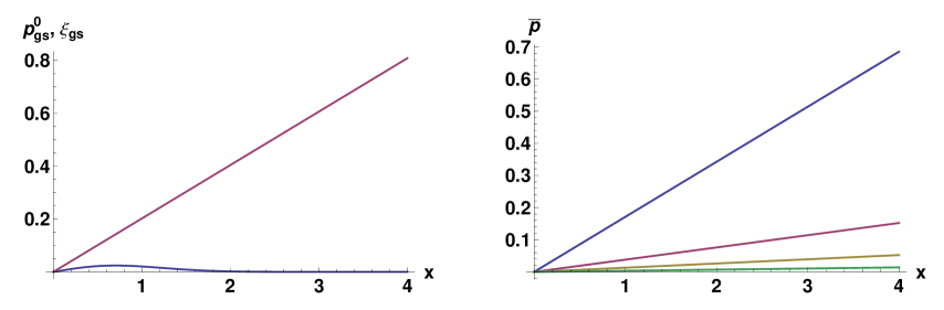
Figure 1: Distribution of electric field $p^{0}_{gs}$ (blue line) and $\xi_{gs}$ (red line) for $\tau=$0 (left), and “slow” electric field $\bar{p}$ (right) for $\tau=2$(blue line), $\tau=8$(red line), $\tau=12$(yellow line), $\tau=18$(green line), and for $b=1.01$, $\varepsilon=0.1$, $\mu=\sqrt{1/2000}$ and $\gamma=0.1$.

As for the spatial dependencies of the average ion velocity and density at the same time moments they are presented on Figure 2.

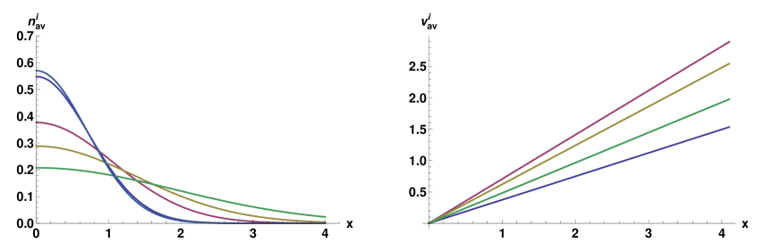
Figure 2: Averaged density and velocity distributions of ions for $\tau=0$ (light-blue line), $\tau=2$(dark-blue line), $\tau=8$(red line), $\tau=12$(yellow line), $\tau=18$(green line), and $b=1.01$, $\varepsilon=0.1$, $\mu=\sqrt{1/2000}$, and $\gamma=0.1$.

It follows from (37) that the oscillating electric field is of the order of the average electric field that accelerates ions. In the next section we consider the opposite situation when the initial electric field practically concise with the initial “slow” electric field $\bar{p}$ and the amplitude of the “fast” electric field is small.

5.2 Examples of slow plasma dynamics: Lorentz density profile

Turn now to the case when there is very slight difference between $p^{0}$ and $\xi$ that is realized, for example, for the Lorentz-type initial density distribution,

$$n_{e}^{0}(x)=(1/\pi(1+x^{2}))\,,\quad n_{i}^{0}(x)=(b/\pi(1+b^{2}x^{2}))\,,\quad\mid b-1\mid\,\ll 1\,.$$ (38)

Substitution of (38) into (21) gives the following formulas for the spatial distribution of the initial electric field and the function $\xi$,

$$p^{0}_{l}(x)=\frac{1}{\pi\varepsilon}\left(\arctan bx-\arctan x\right)\,,\quad\xi_{l}=2\varepsilon x\left(\frac{1}{1+x^{2}}+\frac{\gamma^{2}b^{2}}{1+b^{2}x^{2}}\right)\,.$$ (39)

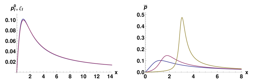
Figure 3: Plots of $p^{0}_{l}$ (blue line) and $\xi_{l}$ (red line) at $\tau=$ 0 (left), and “slow” electric field $\bar{p}$ (right) at $\tau=$ 4 (blue line), $\tau=$ 10 (yellow line), $\tau=$ 18 (red line), for $a=1.0$, $b=1.0661$, $\varepsilon=0.1$, $\mu=\sqrt{1/2000}$ and $\gamma=0.001$.

The left panel of Figure 3 demonstrates the difference between $p^{0}_{l}$ and $\xi_{l}$, and the right panel shows the spatial distribution of the “slow” electric field $\bar{p}$ at different moments of time $\tau$.

As for the average ion density, temperature and velocity they are given by the formulas

$$n^{i}_{av}=\frac{b}{\pi(1+b^{2}{x^{\prime}}^{2})}\frac{{\xi}^{\prime}_{l}}{{\bar{\xi}_{l}}}\,,\ T^{i}=T^{i}_{0}\left(\frac{{\xi}^{\prime}_{l}}{{\bar{\xi}_{l}}}\right)^{2}\,,\ v^{i}_{av}=\frac{1}{\bar{\xi}_{l}\sqrt{2\varepsilon}}\int_{x^{\prime}}^{\bar{x}}{\rm d}y\left(\int_{x^{\prime}}^{y}{\rm d}z/{\xi}^{\,3}_{l}\right)^{-1/2}\,.$$ (40)

and are plotted on the Figure 4.

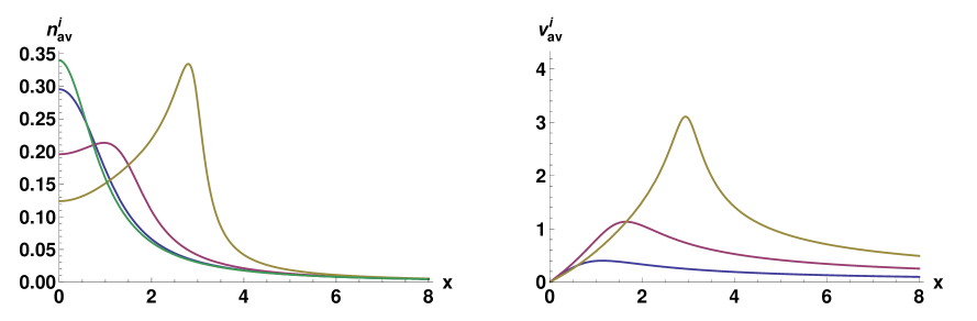
Figure 4: Density and velocity distributions for ions at $\tau=$ 0 (green line), $\tau=$ 4 (blue line), $\tau=$ 10 (red line), $\tau=$ 18 (yellow line), for $b=1.0661$, $\varepsilon=0.1$, $\mu=\sqrt{1/2000}$ and $\gamma=0.001$.

6 Fast dynamics of particles

In this section we use slow invariants to restore the complete dynamics of fast particles, electrons. For clarity’s sake we consider the case of small values of $\delta\varepsilon\ll 1$, which means that $x$ is identical to $\bar{x}$, and rewrite the Lie equations (26) in a simplified form

$$\frac{dt}{da}=1+\varepsilon\tau^{2}\partial_{x}\xi\,,\quad\frac{d(\xi u)}{da}=\delta\xi\cos\Omega t\,,\quad\frac{d(\xi^{3}p)}{da}=\delta\Omega\xi^{3}\cos\Omega t\,.$$ (41)

According to the procedure of averaging [3] we can write the solutions of equations (41) by integrating over fast time $t$ and taking into account the dependence upon slow time by including the dependence upon $\bar{x}$ and $\tau$ into $\delta$ and $\xi$. However, the enhanced precision is achieved by direct integration of the Lie equations (41) in account of the slow dependence of $\tau$ upon $\bar{x}$ as given by slow motion invariants

$$p=\frac{{{\xi}^{\prime}}^{3}}{{\bar{\xi}}^{3}}{\bar{p}}^{\,\prime}+\frac{1}{{\bar{\xi}}^{3}}\int\limits_{x^{\prime}}^{x}{\rm d}x^{\prime\prime}\frac{\bar{\delta}{\bar{\Omega}}{\xi}^{2}(x^{\prime\prime})}{\varepsilon\mu\tau(x^{\prime\prime})}\sin({\bar{\Omega}}t(x^{\prime\prime}))\,,$$ (42)

$$u=\frac{{\xi}^{\prime}}{{\bar{\xi}}}{\bar{u}}^{\,\prime}+\frac{1}{{\bar{\xi}}}\int\limits_{x^{\prime}}^{x}{\rm d}x^{\prime\prime}\frac{\bar{\delta}}{\varepsilon\mu\tau(x^{\prime\prime})}\cos({\bar{\Omega}}t(x^{\prime\prime}))\,.$$

Electron distribution function $g=g^{\prime}\equiv g^{0}(x^{\prime},u^{\prime})$ is the invariant of group transformations. Thus substituting $x={\bar{x}}$ and $u^{\prime}$ from (42) in $g^{0}$ and integrating over the velocity $u$ gives the integral characteristic, the average electron velocity and density

$$n^{e}_{av}={n}^{e}_{0}(x^{\prime})\left({\xi}^{\prime}/{\bar{\xi}}\right)\,,\quad u^{e}_{av}=\frac{1}{\xi^{\prime}}\int\limits_{x^{\prime}}^{x}{\rm d}x^{\prime\prime}\frac{\bar{\delta}}{\varepsilon\mu\tau(x^{\prime\prime})}\cos({\bar{\Omega}}t(x^{\prime\prime}))\,.$$ (43)

To illustrate these formulas we employ results of the previous section and consider the Lorentz-type initial densities profiles (38) with the function $\xi=\xi_{l}$ defined by (39). Substituting $\xi_{l}$ in (42)–(43) we obtain the formulas for the spatial distribution of the electric field and the average electron velocity that are presented on the figures below for three different time moments. Figure 5 corresponds to moderate values of $\tau=4$, when the ion density is concentrated mainly in the center of the bunch thus leading to small-scale spatial oscillations primarily in this region.

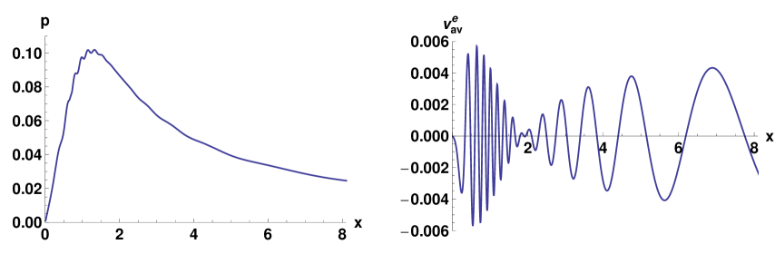
Figure 5: Electric field and average electron velocity distributions at $\tau=4$ for $a=1.0$, $b=1.0661$, $\varepsilon=0.1$, $\mu=\sqrt{1/2000}$ and $\gamma=0.001$.

As the bunch spreads with growth of $\tau$ the small-scale spatial oscillations moves outward as shown on Figure 6 for $\tau=10$,

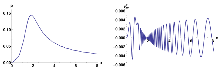
Figure 6: Electric field and average electron velocity distributions at $\tau=10$ for $a=1.0$, $b=1.0661$, $\varepsilon=0.1$, $\mu=\sqrt{1/2000}$ and $\gamma=0.001$.

and on Figure 7 for $\tau=18$. The figures also show that the “complete” electric field $p$ in this case oscillates with the same spatial period as the mean electron velocity and only slightly differs from the average electric field $\bar{p}$ (compare with Figures 3).

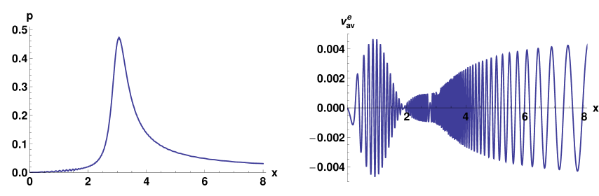
Figure 7: Electric field and average electron velocity distributions at $\tau=18$ for $a=1.0$, $b=1.0661$, $\varepsilon=0.1$, $\mu=\sqrt{1/2000}$ and $\gamma=0.001$.

7 Conclusion

In the above analysis of a particular physical problem, expansion of a plasma bunch, a new promising tool for analyzing nonlinear multi-scale systems was considered. The main idea consists in employing the Krylov-Bogoliubov-Mitropolskii procedure of averaging to construct solutions of Lie equations. The procedure of separating “fast” and “slow” terms in coordinates of group generator naturally occurs in determining equations while constructing the symmetry for nonlinear equations that describe multi-scale behavior of any physical system. In our consideration we use the averaging procedure in combination with a perturbation technique of group analysis [8] that gives approximate symmetries for the analyzed problem and helps to construct approximate RG-invariant solution for arbitrary initial distribution functions of particles.

The use of the averaging procedure in modern group analysis naturally separates invariant manifolds, related to slow and fast Lie equations into slow and fast invariant manifolds. This separation is in the root of the theorem of invariant representation [16, §18]: averaging the fast invariant solution that appears as an oscillating “curve” on fast manifold yields a smooth curve on the slow invariant manifold as shown in the previous section (compare to the method of slow invariant manifold for describing kinetics of dissipative systems [17]). The merits of the approach with different scales that simplifies both the procedure of finding the admitted group and construction of the group invariant solutions point to the quest for future potential applications.

References

- [1] A. H. Nayfeh, Perturbation methods (Wiley, New York, 1973).
- [2] V. F. Zhuravlev, D. M. Klymov, Applied methods in the theory of oscillations, (Moscow, “Nauka”, 1988).
- [3] N. N. Bogoliubov and Yu. A. Mitropolsky, Asymptotic methods in the theory of nonlinear oscillations, 4th ed., (“Nauka”, Moscow, 1974; English transl. of 2nd ed., Hindustan, Delhi, 1961, and Gordon & Breach, New York, 1962).
- [4] N. M. Krylov, N. N. Bogolyubov, Introduction to non-linear mechanics (Kiev: Izd-vo AN SSSR, 1937 (in Russian); 1947 (in English, partial translation from Russian). Princeton: Princeton Univ. Press.)
- [5] G. I. Hori, Theory of general perturbations with unspecified canonical variables, Publ. Astron. Soc. Jap. 18 (1966) 287–296.
- [6] Yu. A. Mitropolsky, A. K. Lopatin, A group-theoretic approach in asymptotical methods of nonlinear mechanics, (Naukova Dumka, Kiev, 1988). (English transl.: Nonlinear mechanics, groups and symmetry. Mathematics and its Applications, 319. Kluwer Academic Publishers Group, Dordrecht, 1995.)
- [7] V. A. Baikov, R. K. Gazizov, N. H. Ibragimov, Method of multiple scales in approximate group analysis: Boussinesq and Korteweg-de-Vries equations (Moscow: Nat. Cent. Math. Model., 1991, preprint No.31 (in Russian)).
- [8] V. A. Baikov, R. K. Gazizov, N. H. Ibragimov, Approximate symmetries, Math. USSR Sb 64(2) (1989) 427–441.
- [9] V. F. Kovalev, S. V. Krivenko, and V. V. Pustovalov, Group analysis of the Vlasov kinetic equation, I, II, Differential Equations 29(10) (1993) 1568–1578; ibid 29(11) (1993) 1712–1721.
- [10] V. F. Kovalev, D. V. Shirkov, Renormalization-group symmetries for solutions of nonlinear boundary value problems, Physics Uspekhi 51(8) (2008) 815–830.
- [11] V. B. Taranov, On the symmetry of one-dimensional high-frequency motions of a collisionless plasma, Journal of Technical Physics 46 (1976) 1271–1277 [in Russian].
- [12] Y. N. Grigoriev, S. V. Meleshko, Group analysis of the integro–differential Boltzman equation, Dokl. AS USSR 297(2) (1987) 323–327.
- [13] Y. N. Grigoriev, S. V. Meleshko, Group analysis of kinetic equations, Russian J. Numer. Anal. Math. Modelling 10(5) (1995) 425–447.
- [14] V. F. Kovalev, V. Yu. Bychenkov, and V. T. Tikhonchuk, Particle dynamics during adiabatic expansion of a plasma bunch, Journ. Exper. Theor. Physics, 95(2) (2002) 226 -241.
- [15] Yu. N. Grigoriev, N. H. Ibragimov, V. F. Kovalev, S. V. Meleshko, Symmetries of Integro-Differential Equations, Series: Lecture Notes in Physics, Vol. 806 (Springer, Berlin/Heidelberg, 2010).
- [16] L. V. Ovsyannikov, Gruppovoi Analiz Differentsial’nykh Uravnenii (Group Analysis of Differential Equations) (Moscow: Nauka, 1978) [Translated into English (New York: Academic Press, 1982)]
- [17] A. N. Gorban, I. V. Karlin, Invariant Manifolds for Physical and Chemical Kinetics, Series: Lecture Notes in Physics, Vol. 660 (Springer, Berlin/Heidelberg, 2005).