Trapping photon-dressed Dirac electrons in a quantum dot studied by coherent two dimensional photon echo spectroscopy

Abstract

We study the localization of dressed Dirac electrons in a cylindrical quantum dot (QD) formed on monolayer and bilayer graphene by spatially different potential profiles. Short lived excitonic states which are too broad to be resolved in linear spectroscopy are revealed by cross peaks in the photon-echo nonlinear technique. Signatures of the dynamic gap in the two-dimensional spectra are discussed. The effect of the Coulomb induced exciton-exciton scattering and the formation of biexciton molecules are demonstrated.

I Introduction

Due to its unique band structure, the charge carriers in graphene are massless Dirac fermions which can cross high potential barriers with ideal unity transmission coefficient (the Klein paradox) castro2009electronic . This ensures a very effective escape channel from a trapping potential thus making it hard for conventional Dirac electrons to be localized within graphene based QDs. Within a finite spatial region defined by sharp potential profile xavier2010topological ; paananen2011signatures ; pal2011electric ; park2010tunable ; matulis2008quasibound ; wunsch2008electron ; hewageegana2008electron . To overcome this difficulty, and trap the electrons for sufficiently long time, we propose to dress the electrons with circularly polarized photons, thus providing them with an effective masskibis2010metal ; pal2011electric . The localization is demonstrated in a cylindrical quantum dot (QD) formed in monolayer and bilayer graphene by antisymmetric potential kink. Conventionally the measure of localization are characteristic resonances in the electronic density of stateswunsch2008electron ; hewageegana2008electron . The dynamical gap is studied semi-classically using Floquet’s theorem zhou2011optical . We present a fully quantum mechanical model, which is based on dressing electrons in monolayer and bilayer configurations. Our calculations show that the dressing not only opens up a dynamical gap in the energy dispersion but also renormalizes the Fermi velocity and inter layer coupling coefficients. In the bilayer configuration, the dressing tunes the gap. That is, it can either close or open the gap, depending on the polarity of the potential kink and the direction/degree of the polarization. The resulting confined electronic states should have similarities with the surface states of topological insulators. Their energies are located inside the energy gap and the wave functions decay away from the interface of the kink potential. These topological states, with the carriers propagating along the potential kink, are expected to be robust with respect to the effects of disorder xavier2010topological . The fully localized states are mixed with the quasi-bound states above the energy gap which can effectively carry away the energy. Conventional linear response spectra (proportional to the density of states) provides limited information about them due to the large broadening caused by their short lifetime hewageegana2008electron . We propose to utilize femtosecond nonlinear spectroscopy in order to study their dynamics. We shall use a four-wave mixing technique known as photon-echoabramavicius2009coherent . The mixed signal is heterodyne detected in the direction of $-\mathbf{k}_{1}+\mathbf{k}_{2}+\mathbf{k}_{3}$ as shown in Fig. 4. The photon echo is known to be able to eliminate the inhomogeneous broadening due to impurities, and allow us to focus on the intrinsic lifetimes of the electronic states. We further discuss signatures of the dynamic gap on the two-dimensional (2D) spectra. There is yet another peculiar characteristic of localized Dirac electrons. As in metals, they are dynamically screened, leading to small Coulomb interaction between them. For small QD this leaves Pauli blocking as the primary source of the nonlinear signalwunsch2008electron . This allows us to calculate it as a sum-over-states (supermolecule) formalism. We can further simplify the signal interpretation by switching to the quasiparticle picture. Those are given as deviation from ideal bosonsabramavicius2009coherent for which the nonlinear signals vanishes. We are able to consider only excited states absorption Liouville pathways without contribution from the ground state bleaching and excited states emission. This interference reduction provides relatively simple interpretation of the 2D spectra. The short lived states can be visualized via the coherences (off-diagonal cross resonances) with those fully localized. We employ visible light to map the QD interband transitions onto the 2D spectra. Finally we briefly discuss the effect of the Coulomb induced exciton scattering based on nonlinear exciton equationskavousanaki2009probing . Possible formation of biexciton molecules is demonstrated.

The outline of this paper is as follows. In Sec. II, we present the model Hamiltonian for graphene irradiated with a circularly polarized electromagnetic field. Section III is devoted to dressing of electrons in bilayer graphene and a derivation of the eigenstates. We deal with the trapping of the dressed electrons within a QD in Sec. IV. Section V presents the absorption and correlation spectrum for dressed electrons in a QD. We present numerical results in Sec. VI and conclude in Sec. VI with a summary of our results.

II Dressed electrons in free standing graphene.

The electronic Hamiltonian of graphene irradiated with an electromagnetic field may be expressed askibis2010metal :

$$\mathcal{H}=\mathcal{H}_{0}+\mathcal{H}_{1}+\mathcal{H}_{2}$$ (1)

$$\mathcal{H}_{0}=\hbar\omega_{0}a^{\dagger}_{0}a_{0}+\frac{W_{0}}{\sqrt{N_{0}}}\left({\sigma_{+}a_{0}+\sigma_{-}a_{0}^{\dagger}}\right)$$ (2)

$$\mathcal{H}_{1}=\hbar v_{F}\bm{\sigma}\cdot\mathbf{k}+\mathcal{I}V(x,y)$$ (3)

$$\mathcal{H}_{2}=\sum\limits_{i=1}^{\infty}\hbar\omega_{i}a^{\dagger}_{i}a_{i}+\frac{W_{i}}{\sqrt{N_{i}}}\left({(\sigma_{+}+\sigma_{-})(a_{i}+a^{\dagger}_{i})}\right)\ .$$ (4)

Here, $\mathcal{H}_{0}$ describes the Jaynes-Cummings modelgerry2003introduction with $a_{0}$ being the annihilation operator of a single mode circularly polarized optical field with frequency $\omega_{0}$ and $N_{0}$ photons in the mode. Each of them carries the energy $\hbar\omega_{0}$. $\sigma_{\pm}=(\sigma_{x}\pm i\sigma_{y})/2$ are raising and lowering operators for $z-$ projection of the electrons pseudo-spin. In matrix representation these are Pauli matrices. $W_{0}/\sqrt{N_{0}}$ is the electron-photon coupling, a quantum mechanical analogue of the classical rotational motion caused by the circularly polarized wave.

$\mathcal{H}_{1}$ describes conventional Dirac Hamiltoniancastro2009electronic of graphene with Fermi velocity $v_{F}=10^{6}\;m/s$; $\mathbf{k}$ is the wave vector measured from one of the $\mathbf{K}$ points, $V(x,y)$ is an external QD confining potential; $\mathcal{I}$ is the identity matrix. $\mathcal{H}_{2}$ describes the rest of the optical modes latter used to probe the dressed states by four-wave mixing process.

The Hamiltonian $\mathcal{H}_{0}$ may be diagonalized in a straightforward way gerry2003introduction in the following basis:

$$|{\psi_{N_{0}}}\rangle=\left({\begin{array}[]{c}|{\psi_{+,N_{0}}}\rangle\\ |{\psi_{-,N_{0}}}\rangle\end{array}}\right)\ ,$$ (7)

$$|{\psi_{\pm,N_{0}}}\rangle=\cos\phi|{\pm,N_{0}}\rangle\pm\sin\phi|{\mp,N_{0}\pm 1}\rangle$$ (8)

$$\cos\phi=\sqrt{\frac{\Omega_{N_{0}}+\hbar\omega_{0}}{2\Omega_{N_{0}}}}$$ (9)

$$\sin\phi=\sqrt{\frac{\Omega_{N_{0}}-\hbar\omega_{0}}{2\Omega_{N_{0}}}}$$

$$\Omega_{N_{0}}=\hbar\omega_{0}+W_{0}^{2}(N_{0}+1)/N_{0}\ .$$ (10)

Here, the direct product state $|{\pm,N_{0}\rangle}$ define the uncoupled electron with pseudo spin up (+) or down (-) and the optical mode with $N_{0}$photons. Eq. (8) defines the dressed electron states. In the basis of Eq. (7), the Jaynes-Cummings Hamiltonian assumes the form

$$\langle{\psi_{N_{0}}}|\mathcal{H}_{0}|{\psi_{N_{0}}}\rangle$$ (11)

$$=\left({\begin{array}[]{cc}\langle{\psi_{+,N_{0}}}|\mathcal{H}_{0}|{\psi_{+,N_{0}}}\rangle&\langle{\psi_{+,N_{0}}}|\mathcal{H}_{0}|{\psi_{-,N_{0}}}\rangle\\ \langle{\psi_{-,N_{0}}}|\mathcal{H}_{0}|{\psi_{+,N_{0}}}\rangle&\langle{\psi_{-,N_{0}}}|\mathcal{H}_{0}|{\psi_{-,N_{0}}}\rangle\end{array}}\right)$$ (14)

$$=\left({\begin{array}[]{cc}N_{0}\hbar\omega_{0}+E_{g}/2&0\\ 0&N_{0}\hbar\omega_{0}-E_{g}/2\end{array}}\right)$$ (17)

$$=\mathcal{I}N_{0}\hbar\omega_{0}+(E_{g}/2)\sigma_{3}\ .$$

The first term is a constant, and may be omitted.

The remaining Hamiltonian matrix elements are calculated in Appendix B, yielding

$$\langle{\psi_{N_{0}}}|\mathcal{H}_{1}|{\psi_{N_{0}}}\rangle=\hbar\tilde{v}_{F}\bm{\sigma}\cdot\mathbf{k}+\mathcal{I}V(x,y)$$ (18)

$$\langle{\psi_{N_{0}}}|\mathcal{H}_{2}|{\psi_{N_{0}}}\rangle=$$ (19)

$$\sum\limits_{i=1}^{\infty}\mathcal{I}\hbar\omega_{i}a^{\dagger}_{i}a_{i}+\frac{\tilde{W}_{i}}{\sqrt{N_{i}}}\left({(\sigma_{+}+\sigma_{-})(a_{i}+a^{\dagger}_{i})}\right)\ ,$$

where $\tilde{v}_{F}\equiv v_{F}\cos^{2}\phi$ is the renormalized Fermi velocity and $\tilde{W}_{i}\equiv W_{i}\cos^{2}\phi$ are the renormalized couplings to the probing optical modes.

In the absence of a potential ($V(x,y)=0$), the eigenvalues of $\mathcal{H}_{0}+\mathcal{H}_{1}$ are $\pm\sqrt{(\hbar\tilde{V}_{F}k)^{2}+(E_{g}/2)^{2}}$ and the corresponding eigenfunctions are:

$$\Psi_{+}(k)=\texttt{e}^{i\mathbf{kr}}\left({\begin{array}[]{c}\cos\left({\alpha_{k}/2}\right)\\ \texttt{e}^{i\beta_{k}}\sin\left({\alpha_{k}/2}\right)\end{array}}\right)$$ (22)

$$\Psi_{+}(k)=\texttt{e}^{i\mathbf{kr}}\left({\begin{array}[]{c}\sin\left({\alpha_{k}/2}\right)\\ -\texttt{e}^{i\beta_{k}}\cos\left({\alpha_{k}/2}\right)\end{array}}\right)$$ (25)

$$\texttt{Tan}\beta_{k}=k_{y}/k_{x};$$ (26)

$$\texttt{Tan}\alpha_{k}=2\hbar\tilde{v}_{F}k/E_{g}\ .$$

III Dressed electrons in bi-layer graphene

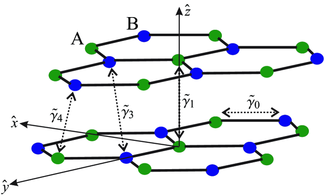
Figure 1: Bilayer graphene structure and renormalized coupling coefficients.

Starting with Eq. (38) of the review article of Castro Neto, et al. castro2009electronic , and applying the procedure of Appendix A, the Hamiltonian which describes the dressing of the electrons in the bilayer (Bernal stack) can be expressed as

$$H=\left({\begin{array}[]{cc}H_{11}&H_{12}\\ H_{21}&H_{22}\end{array}}\right)$$ (29)

Here $H_{11}=\mathcal{H}(V_{1})$ and $H_{22}=\mathcal{H}(V_{2})$ describe the electrons on the first and second graphene layers respectively. Those layers may experience different potential profiles $(V_{1,2})$ entering Eq. (3). The interlayer coupling is described by the off-diagonal block matrices as:

$$H_{12}=\gamma_{1}\sigma_{-}+3\gamma_{3}a(k_{x}-ik_{y})\sigma_{+}$$ (30)

$$+\frac{W^{3}_{0}}{\sqrt{N_{0}}}\sigma_{+}a_{0}+\sum\limits_{i=1}\frac{W^{3}_{i}}{\sqrt{N_{i}}}(\sigma_{+}+\sigma_{-})(a_{i}+a^{\dagger}_{i})$$

$$H_{21}=\gamma_{1}\sigma_{+}+3\gamma_{3}a(k_{x}+ik_{y})\sigma_{-}$$ (31)

$$+\frac{W^{3}_{0}}{\sqrt{N_{0}}}\sigma_{-}a^{\dagger}_{0}+\sum\limits_{i=1}\frac{W^{3}_{i}}{\sqrt{N_{i}}}(\sigma_{+}+\sigma_{-})(a_{i}+a^{\dagger}_{i})\ .$$

Here, we have introduced effective electron-photon coupling matrix elements $W^{j}_{i}/\sqrt{N_{i}}=-3e\gamma_{j}a\sqrt{2\pi/\omega_{i}\Omega\hbar}$, where $a=1.42$ Å  is the carbon-carbon distance within a layer. Additionally, we have $\gamma_{0}=2.8\ ,\texttt{eV}$ is the nearest-neighbor hopping energy within the layer $(A_{1}\rightleftharpoons B_{1},A_{2}\rightleftharpoons B_{2})$. Fermi velocity can be expressed in terms of the above parameters as $\hbar v_{F}=3\gamma_{0}a/2$. $\gamma_{1}=0.4\;\texttt{eV}$ is the inter-layer hopping energy between atoms of type A: $(A_{1}\rightleftharpoons A_{2})$. $\gamma_{3}=0.3\;\texttt{eV}$ is the inter-layer hopping energy between atoms of type B: $(B_{1}\rightleftharpoons B_{2})$. $\gamma_{4}=0.04\;\texttt{eV}$ is the inter-layer hopping energy between atoms of type B and A: $(A_{1}\rightleftharpoons B_{2},B_{1}\rightleftharpoons A_{2})$. Electronic couplings between various atoms in the bilayer graphene are shown in Fig. 1. The double layer can be regarded as corresponding to as $\gamma_{1}=\gamma_{3}=\gamma_{4}=0$.

In the dressed state basis of Eq. (99), the diagonal blocks are given by the results of the previous section as

$$\langle{\psi_{N_{0}}}|H_{11,22}|{\psi_{N_{0}}}\rangle$$ (32)

$$=\hbar\tilde{v}_{F}\bm{\sigma}\cdot\mathbf{k}+(E_{g}/2)\sigma_{3}+\mathcal{I}V_{1,2}(x,y)$$

$$+\mathcal{I}N_{0}\hbar\omega_{0}+\sum\limits_{i=1}\mathcal{i}\hbar\omega_{i}a^{\dagger}_{i}a_{i}+\frac{\tilde{W}^{0}_{i}}{\sqrt{N_{i}}}(\sigma_{+}+\sigma_{-})(a_{i}+a^{\dagger}_{i})\ .$$

The off-diagonal blocks may be derived from Eqs. (30), (31) and Appendix C to become:

$$\langle{\psi_{N_{0}}}|H_{12}|{\psi_{N_{0}}}\rangle=\tilde{\gamma}_{1}\sigma_{-}+3\tilde{\gamma}_{3}a(k_{x}-ik_{y})\sigma_{+}$$ (33)

$$+\tilde{\gamma}_{4}\sigma_{3}+\sum\limits_{i=1}\frac{\tilde{W}^{3}_{i}}{\sqrt{N_{i}}}(\sigma_{+}+\sigma_{-})(a_{i}+a^{\dagger}_{i})$$

$$\langle{\psi_{N_{0}}}|H_{21}|{\psi_{N_{0}}}\rangle=\tilde{\gamma}_{1}\sigma_{+}+3\tilde{\gamma}_{3}a(k_{x}+ik_{y})\sigma_{-}$$ (34)

$$+\tilde{\gamma}_{4}\sigma_{3}+\sum\limits_{i=1}\frac{\tilde{W}^{3}_{i}}{\sqrt{N_{i}}}(\sigma_{+}+\sigma_{-})(a_{i}+a^{\dagger}_{i})\ ,$$

where the renormalized model parameters are $\tilde{\gamma}_{1,2}=\gamma_{1,2}\cos^{2}\phi$, $\tilde{\gamma}_{4}=(W^{3}_{0}/2)\sin 2\phi$ and $\tilde{W}^{3}_{i}=W^{3}_{i}\cos^{2}\phi$. For the purpose of further discussion, it is convenient to localize $H_{0}+H_{1}$ as we did in a preceding section for monolayer graphene. The corresponding matrix elements are

Single layer:

$$\langle{\psi_{N_{0}}}|\langle{B_{1}A_{1}}|\mathcal{H}_{0}+\mathcal{H}_{1}|{A_{1}B_{1}}\rangle|{\psi_{N_{0}}}\rangle$$ (35)

$$=\left({\begin{array}[]{cc}V_{1}(x,y)+(E_{g}/2)&\frac{3}{2}\tilde{\gamma}_{0}a(k_{x}+ik_{y})\\ \frac{3}{2}\tilde{\gamma}_{0}a(k_{x}-ik_{y})&V_{1}(x,y)-(E_{g}/2)\end{array}}\right)$$ (38)

Bilayer:

$$\langle{\psi_{N_{0}}}|\langle{B_{2}A_{2}A_{1}B_{1}}|H_{0}+H_{1}|{B_{1}A_{1}A_{2}B_{2}}\rangle|{\psi_{N_{0}}}\rangle$$ (39)

$$=\left({\begin{array}[]{cccc}V_{1}(x,y)+(E_{g}/2)&\frac{3}{2}\tilde{\gamma}_{0}a(k_{x}+ik_{y})&\tilde{\gamma}_{4}&3\tilde{\gamma}_{3}a(k_{x}-ik_{y})\\ \frac{3}{2}\tilde{\gamma}_{0}a(k_{x}-ik_{y})&V_{1}(x,y)-(E_{g}/2)&\tilde{\gamma}_{1}&-\tilde{\gamma}_{4}\\ \tilde{\gamma}_{4}&\tilde{\gamma}_{1}&V_{2}(x,y)+(E_{g}/2)&\frac{3}{2}\tilde{\gamma}_{0}a(k_{x}-ik_{y})\\ 3\tilde{\gamma}_{3}a(k_{x}+ik_{y})&-\tilde{\gamma}_{4}&\frac{3}{2}\tilde{\gamma}_{0}a(k_{x}+ik_{y})&V_{2}(x,y)-(E_{g}/2)\end{array}}\right)\ .$$ (44)

This implies that the dressing of the Dirac electrons in bilayer gives

• renormalized interlayer coupling coefficients, which are denoted by tilde.,

• broken the symmetry between the sub-lattices $(A_{1},B_{1};A_{2},B_{2})$ of each of the layers. Measure of the broken symmetry is $(E_{g}/2)$,

• broken symmetry between the sub-lattices $(A_{1},B_{2};A_{2},B_{1})$ belonging to different layers. A measure of the broken symmetry is $\tilde{\gamma}_{4}$.

The corresponding eigenvalues for constant potentials ($V_{1},V_{2}$) are shown in Fig. 2 for chosen values of the parameters. We first focus on the largest interlayer coupling $\tilde{\gamma}_{1}$ and neglect the rest of the coupling (Figs. 2(a)). The four bands are given by

$$\left({2E+V_{2}+V_{1}}\right)^{2}$$ (45)

$$=E_{g}^{2}+\left({V_{1}-V_{2}}\right)^{2}+9a^{2}k^{2}\tilde{\gamma}^{2}_{0}+2\tilde{\gamma}_{1}^{2}\pm 2\sqrt{\left({V_{1}-V_{2}}\right)^{2}\left({E^{2}_{g}+9a^{2}k^{2}\tilde{\gamma}^{2}_{0}}\right)+\tilde{\gamma}^{2}_{1}\left({9a^{2}k^{2}\tilde{\gamma}_{0}^{2}-2E_{g}\left({V_{1}-V_{2}}\right)}\right)+\tilde{\gamma}^{4}_{1}}\ .$$

On its own, $E_{g}$ opens a gap in the bilayer spectrum similar to the monolayer (Fig. 2(a.1)). The gap may be opened by applying a potential difference between the layers ($V_{1}\neq V_{2}$ in Fig. 2(a.2)). The combined effect of the potential difference and $E_{g}>0$ can either widen $V_{2}-V_{1}<0$ or shrink $V_{2}-V_{1}>0$ the gap compared with the gap induced by the potential difference itself (Fig. 2(a.3)). We observe that when $2E_{g}=V_{2}-V_{1}$, the gap closes (Fig. 2(a.4)). Inclusion of the rest of the coupling breaks the symmetry between $k_{x}$ and $k_{y}$, as follows from Fig. 1. The analytical form of the energy bands, although possible, is too large to be presented here. The energy bands are shown in Fig. 2(b-d).

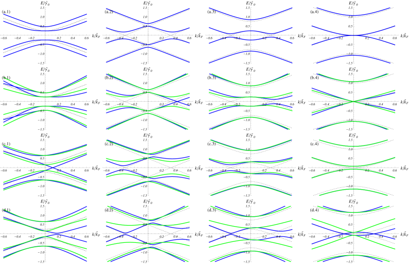
Figure 2: Dotted/solid curves represent electron dispersion of double/bilayer graphene. Panels (a) assume that $\tilde{\gamma}_{1}/\tilde{\gamma}_{0}=0.4$ and the remaining interlayer coupling parameters are zero. Panels (b) also introduce the effect of $\tilde{\gamma}_{3}/\tilde{\gamma}_{0}=0.3$. Panels (c) demonstrate the effect of $\tilde{\gamma}_{4}/\tilde{\gamma}_{0}=0.3$. Panels (d) illustrate the combined effect of $\tilde{\gamma}_{3}$ and $\tilde{\gamma}_{4}$. In columns (1) we have dressing induced $E_{g}/\tilde{\gamma}_{0}=1/2$ with no potential difference between the layers. In columns (2) we potential difference between the layers $(V_{1}-V_{2})/\tilde{\gamma}_{0}=1/2$ with no electron dressing $E_{g}/\tilde{\gamma}_{0}=0$. Columns (3,4) illustrate their combine effect; (3) correspond to $E_{g}/\tilde{\gamma}_{0}=1/2$ and (4) has $E_{g}/\tilde{\gamma}_{0}=1$. Blue (green) curves show a section of the energy along $k_{x}(k_{y})$ directions.

IV Dressed electrons confined in a QD

Let us now turn to the problem of trapping dressed electrons within a QD. Since the confining potential $V_{1}(x,y)$ is radial it is convenient to work with cylindrical coordinates $x=r\cos\theta\;y=r\sin\theta$. This ammounts to the following substitutions:

$$k_{x}=-i\partial_{x},\;k_{y}=-i\partial_{y}$$ (46)

$$\partial_{x}\pm i\partial_{y}=\texttt{e}^{\pm i\theta}\left({\partial_{r}\pm\frac{i}{r}\partial_{\theta}}\right)\ .$$

Thanks to the potential radial symmetry the Hamiltonians in Eq. (35) and (39) commutes with the angular momentum operator $\hat{L}_{z}=\mathcal{I}\left({xk_{y}-yk_{x}}\right)$. Here we have neglected symmetry breaking contributions to the Hamiltonian ($\tilde{\gamma}_{3,4}\ll\tilde{\gamma}_{1}$). Therefore, we may seek solution of the Dirac equation in the form:

$$|{\Psi_{m}(\mathbf{r})}\rangle=\left({\begin{array}[]{c}\psi_{m,B_{1}}(r)\texttt{e}^{i(m+1/2)\theta}\\ i\psi_{m,A_{1}}(r)\texttt{e}^{i(m-1/2)\theta}\\ i\psi_{m,A_{2}}(r)\texttt{e}^{i(m-1/2)\theta}\\ \psi_{m,B_{2}}(r)\texttt{e}^{i(m+1/2)\theta}\end{array}}\right)\ .$$ (47)

Here, the projection of the angular momentum has eigenvalues $m=\pm 1/2,\pm 3/2,\pm 5/2,\ldots$. Substituting Eqs. (47) and (46) into (39), we obtain the following system of ordinary differential equations

$$\left({\begin{array}[]{cccc}V_{1}(r)+(E_{g}/2)&\frac{3}{2}\tilde{\gamma}_{0}a(\partial_{r}-\frac{m-1/2}{r})&0&0\\ -\frac{3}{2}\tilde{\gamma}_{0}a(\partial_{r}+\frac{m+1/2}{r})&V_{1}(r)-(E_{g}/2)&\tilde{\gamma}_{1}&0\\ 0&\tilde{\gamma}_{1}&V_{2}(r)+(E_{g}/2)&-\frac{3}{2}\tilde{\gamma}_{0}a(\partial_{r}+\frac{m+1/2}{r})\\ 0&0&\frac{3}{2}\tilde{\gamma}_{0}a(\partial_{r}-\frac{m-1/2}{r})&V_{2}(r)-(E_{g}/2)\end{array}}\right)\left({\begin{array}[]{c}\psi_{m,B_{1}}(r)\\ \psi_{m,A_{1}}(r)\\ \psi_{m,A_{2}}(r)\\ \psi_{m,B_{2}}(r)\end{array}}\right)=E\left({\begin{array}[]{c}\psi_{m,B_{1}}(r)\\ \psi_{m,A_{1}}(r)\\ \psi_{m,A_{2}}(r)\\ \psi_{m,B_{2}}(r)\end{array}}\right)\ .$$ (48)

First, let us consider the case when there is no coupling between the graphene layers. Assuming that the solution of Eq. (48) has the form of $\sqrt{r}\psi_{m}(r)$ in the regions of constant potential, we obtain

$$\left({\begin{array}[]{c}\psi_{m,B_{1}}(r_{<})\\ \psi_{m,A_{1}}(r_{<})\\ \end{array}}\right)=A\left({\begin{array}[]{c}J_{|{m-1/2}|}\left({\frac{2r_{<}\sqrt{E^{2}-(E_{g}/2)^{2}}}{3\tilde{\gamma}_{0}a}}\right)\\ J_{|{m+1/2}|}\left({\frac{2r_{<}\sqrt{E^{2}-(E_{g}/2)^{2}}}{3\tilde{\gamma}_{0}a}}\right)\\ \end{array}}\right)$$ (53)

$$\left({\begin{array}[]{c}\psi_{m,B_{1}}(r_{>})\\ \psi_{m,A_{1}}(r_{>})\\ \end{array}}\right)=B\left({\begin{array}[]{c}H^{(1)}_{|{m-1/2}|}\left({\frac{2r_{>}\sqrt{(E-V_{1})^{2}-(E_{g}/2)^{2}}}{3\tilde{\gamma}_{0}a}}\right)\\ H^{(1)}_{|{m+1/2}|}\left({\frac{2r_{>}\sqrt{(E-V_{1})^{2}-(E_{g}/2)^{2}}}{3\tilde{\gamma}_{0}a}}\right)\\ \end{array}}\right)\ .$$ (58)

The Bessel function form of the wave function inside of the QD ($V_{1}=0,r=r_{<}\leq R$) is dictated by the fact that the wave function must stay finite at $r=0$. Outside the QD ($V_{1}>0,r=r_{>}\geq R$) the wave function must describe the outgoing wave at large distances ($r_{>}\gg R$). We, therefore, took it to be the Hankel function of first kind. At the boundary of the dot the wave function must be continuous. The energies $E_{m,n}$ of the quasi-stationary states inside of the QD are obtained by solving the following equation:

$$\frac{H^{(1)}_{|{m-1/2}|}\left({k_{>}R}\right)}{H^{(1)}_{|{m+1/2}|}\left({k_{>}R}\right)}=\frac{J_{|{m-1/2}|}\left({k_{<}R}\right)}{J_{|{m+1/2}|}\left({k_{<}R}\right)}\ ;$$ (59)

where we have introduced following notation:

$$k_{>}=\frac{2R\sqrt{(E-V_{1})^{2}-(E_{g}/2)^{2}}}{3\tilde{\gamma}_{0}a}$$

$$k_{<}=\frac{2R\sqrt{E^{2}-(E_{g}/2)^{2}}}{3\tilde{\gamma}_{0}a}$$

Those are shown in Fig. 3 for several chosen values of $E_{g}$. The long living solutions $\texttt{Im}[E]\approx 0$ can be obtained analytically by noticing the following identities for the Hankel function in the limit $z\ll 1$,

$$H^{(1)}_{n}(z)=J_{n}(z)+iY_{n}(z)$$ (60)

$$=\frac{1}{\Gamma(n+1)}\left({\frac{z}{2}}\right)^{n}-i\frac{\Gamma(n)}{\pi}\left({\frac{2}{z}}\right)^{n}\ .$$

It is clear from the above equation that when $E=V_{1}\pm E_{g}/2$ the left hand side of Eq. (59) vanishes. Therefore the real energies of the QD correspond to the zeros of the Bessel function with

$$J_{|{m-1/2}|}\left({\frac{2R\sqrt{E_{m,n}^{2}-(E_{g}/2)^{2}}}{3\tilde{\gamma}_{0}a}}\right)=0\ .$$ (61)

The splitting of the central peak in the density of states (DOS) by the electron dressing should be readily accessible in optical experiments. This will be the subject of the following section.

Figure 3: Energy levels (Blue dots) of a QD formed in a graphene monolayer. Green dots correspond to dressed Dirac electrons. The confining potential is $V_{1}=20$, and the gap $E_{g}=10$ (in units of $2R/3\tilde{\gamma}_{0}a$).

Now let us briefly comment on the QD in the bilayer graphene. Since the dressing of the electrons in the bilayer allows wide manipulation of the gap (See Fig. 2(a.3)) one can dynamically form conventional QDs. That is those which support infinitely living electronic states. There are two possible schematics shown in Fig. In one case the dressing and the substrate induced gap work concurrently and the whole realization of the QD is almost identical to the one we had discussed for the single layer. The only difference is the non-homogeneous potential which forms the dot is the potential between the graphene layers. Such QD can be readily realized by screening of the substrate potential inside of the QD. In the other schematic, the combination of the dressing and the substrate potential closes the gap inside of the QD. The electrons become trapped by the gap outside of the QD. In both cases the analytical solution of Eq. (48) may be obtained by following the procedure outlined in Ref.matulis2008quasibound ; xavier2010topological .

V Absorption and photon-echo spectra of dressed Dirac electrons in a single QD

In this section we investigate several linear and non-linear optical techniques which allow to probe the details of the electronic structure calculated above. The linear absorption mostly reveals the long living states ($\texttt{Im}[E]\ll\texttt{Re}[E]$) which show up a narrow resonance and directly reflects the structure of the DOShewageegana2008electron ; wunsch2008electron . Nonlinear photon-echomukamel1995principles signal ( $\chi^{(3)}(-\mathbf{k}_{1}+\mathbf{k}_{2}+\mathbf{k}_{3})$) will be designed to reveal the other short living states. The schematic of the heterodyne detected four wave mixing experiment is shown in Fig. 4 By probing the coherence between the electronic states in the QD, the technique can reveal the energy of the short living electronic quasi-bound states. We shall restrict the discussion to singly excited states, thereby neglecting underlying many-body effects. This allows for a conceptually simple description in terms of the many body eigenstatesabramavicius2009coherent ; mukamel2007sum .

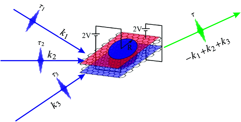
Figure 4: Schematic illustration of the photon-echo technique designed to study the exciton scattering dynamics in graphene based QDs.

It is also possible to study several excitonic states of the QD and their dynamics by applying special nonlinear measurements. We shall also make use of the double quantum coherencemukamel2007sum ($\chi^{(3)}(\mathbf{k}_{1}+\mathbf{k}_{2}-\mathbf{k}_{3})$) technique in order to observe many body effects in biexciton manifold of graphene QD. Conceptually the approach is similar to that described in Ref.chernyak1998multidimensional ; kavousanaki2009probing . However the graphene based QD has large screening of the Coulomb interaction between excitons. Thus it can be safely omitted in the following discussion. Recently the collinear version of $\chi^{(3)}$ technique based on phase-cycling gained popularity in QD studies of terahertz regimekuehn2011strong . Its application to graphene will be reported elsewhere.

Let us first define the effective single particle diagonalized Hamiltonian in the QDmukamel2007sum :

$$\hat{\mathcal{H}}=\sum\limits_{m1,n1}E_{m1}\delta_{m1,n1}\hat{c}^{\dagger}_{m1}\hat{c}_{n1}$$ (62)

$$+\sum\limits_{m2,n2}E_{m2}\delta_{m2,n2}\hat{d}^{\dagger}_{m2}\hat{d}_{n2}$$

• whose matrix elements are obtained from Eq. (59). Each subscript is a composite of two indices describing angular ($m$) and radial ($n$) quantum numbers $m1(2)=\left\{{m,n}\right\}$. Here we have partitioned the electronic states into occupied ($n<0$) and unoccupied ($n>0$) in the ground state obtained by setting up the chemical potential to $\mu=N_{0}\hbar\omega_{0}$. The electrons in the unoccupied state can be created by action of $\hat{c}^{\dagger}_{m1}=|{\Psi_{m,n>0}}\rangle\otimes\langle{\Psi_{m,n<0}}|$ operator on the ground state. Its hermitian conjugate $\hat{c}_{m1}$ removes the electron from that state. Similarly the second term of Eq.  (62) describes the creation $\hat{d}^{\dagger}_{m2}=|{\Psi_{m,n<0}}\rangle\otimes\langle{\Psi_{m,n>0}}|$ and annihilation $\hat{d}_{m2}$ of the electrons in the originally occupied states (holes). The second term in Eq.  (62) is just hermitian conjugate of the first. In the notation above symbol $\otimes$ stands for element-wise multiplication of the vectors. Since the dressing circularly polarized CW mode has been already incorporated in Eq.  (62) we only have to explicitly treat the interaction with the narrow pulsed time ordered incoming and detected modes. This is given by the effective interaction Hamiltonian in rotating wave approximation:

$$\hat{\mathcal{H}}_{\texttt{int}}(t)=\sum\limits_{i,m1,m2}\sum\limits_{j=\pm}\mathcal{E}^{j}_{i}\delta(t-t_{i})\mu^{j}_{m1,m2}\hat{d}_{m2}\hat{c}_{m1}+\texttt{H.c}$$ (63)

• Here $\mathcal{E}^{\star,\pm}_{i}$ stands for the left(right) $\pm$ polarized component of the incoming or detected mode electric field amplitude. The dipole moments of transitions (in units of $\tilde{W}_{i}/(\mathcal{E}^{\pm}_{i}\sqrt{N_{i}})$) are:

$$\mu^{\pm}_{m1,m2}=\int d\mathbf{r}\langle{\Psi_{m1}(\mathbf{r})}|r\texttt{e}^{\pm i\theta}|{\Psi_{m2}(\mathbf{r})}\rangle$$ (64)

• Note that we are still in the single electron-hole representation, not yet in the many body exciton/hole representation. Therefore we do not need the envelop function to define the transition moments as in Ref. agranovich1992electrodynamics .

The next step is to bring the Hamiltonian in Eq. (62),(63) into the excitonic form. Using the method first proposed in Ref.chernyak1998multidimensional we define the electron-hole pair annihilation operators (not to be confused with exciton operators) as:

$$\hat{B}^{{\dagger}}_{m}=\hat{B}_{m1,m2}=\hat{c}_{m1}d_{m2}$$ (65)

• where we used composite index of $m=\left\{{m1,m2}\right\}$ Since we are interested in the third-order response the commutator of the above operators may be truncated at quadratic order:

$$\left[{\hat{B}_{m},\hat{B}^{\dagger}_{n}}\right]=\delta_{m,n}-2\sum_{p,q}\delta_{m,n;p,q}\hat{B}^{\dagger}_{p}\hat{B}_{q}$$ (66)

• where $\delta_{m,n}=\delta_{m1,n1}\delta_{m2,n2}$. The tetradic matrix $\delta_{m,n;p,q}$ (phase-filling factor) is responsible for the deviation from the boson statistic of the pair operators, and steams from the fermionic nature of its constituents:

$$2\delta_{m,n;p,q}$$ (67)

$$=\delta_{m1,q1}\delta_{m2,p2}\delta_{n1,p1}\delta_{n2,q2}+\delta_{m1,p1}\delta_{m2,q2}\delta_{n1,q1}\delta_{n2,p2}$$

• In the basis of electron-hole pairs the Hamiltonian in Eqs.  (61), (62) becomes Frenkel-like if truncated up to forth order(valid for third order response with two excited electron-hole pairs):

$$\hat{\mathcal{H}}=\sum\limits_{m}E_{m}\hat{B}^{\dagger}_{m}\hat{B}_{m}+\frac{1}{4}\sum\limits_{m,n}\left({E_{m}+E_{n}}\right)\hat{B}^{\dagger}_{m}\hat{B}^{\dagger}_{n}\hat{B}_{m}\hat{B}_{n}$$ (68)

$$\hat{\mathcal{H}}_{\texttt{int}}(t)=\sum\limits_{i,m}\sum\limits_{j=\pm}\mathcal{E}^{j}_{i}\delta(t-t_{i})\mu^{j}_{m}\hat{B}_{m}+\texttt{H.c}$$ (69)

• Direct diagonalization of the above Hamiltonian (68) in order to find the exciton/biexciton manifolds is difficult and non-equilibrium Green’s functions for the single and double electron-hole pairs are used instead. If one neglects the nonlinearities caused by the Pauli exclusion those retarded Green’s functions are defined as:

$$G_{e1}(\tau)=-i\theta(\tau)\texttt{e}^{-iE_{e1}\tau}$$ (70)

$$G_{e1,e2}=-i\theta(\tau)\texttt{e}^{-i(E_{e1}+E_{e2})\tau}$$ (71)

Here $\theta(\tau)$ is the Heaviside function and the time between two consecutive pulses is denoted as $\tau_{i}=t_{i+1}-t_{i}$. Note that in order to be retarded the Green’s functions must contain the energies with $\texttt{Im}[E_{e}]<0$. We also adopted the notation $E_{e1}=E_{m1}+E_{m2}$. We shall also need their Fourier transforms with respect to the time delays:

$$G_{e1}(\omega)=\frac{1}{\omega-E_{e1}}$$ (72)

$$G_{e2,e1}(\omega)=\frac{1}{\omega-E_{e1}-E_{e2}}$$ (73)

In the above Green’s functions the biexciton energies (the poles of Eq. (73)) is simply a sum of the exciton energies. The nonlinear signal from such system vanishes since it represents a collection of harmonic oscillators. The effect of Pauli exclusion in Eq. (68) is usually incorporated by tetradic exciton scattering matrix:

$$\Gamma_{e4,e3;e2,e1}(\omega)=\delta_{e4,e3;e2,e1}(G^{-1})_{e4,e3}$$ (74)

Which carries all the information about underlying nonlinearities. Coulomb interaction can be incorporated by solving Bethe-Saltpeter equation as in Ref.mukamel2007sum ; chernyak1998multidimensional ; mukamel1995principles .

The photon echo signal can be recast in terms of non-interacting Green’s functions as well as the scattering matrix as:

$$S^{j1,j2,j3,j4}_{-\mathbf{k}_{1}+\mathbf{k}_{2}+\mathbf{k}_{3}}\left({\omega_{3}},\tau_{2}=0,\omega_{1}\right)$$ (75)

$$=2\texttt{Re}\sum\limits_{e1,e2,e3,e4}\mu^{j1}_{e3}\mu^{\star,j2}_{e2}\mu^{\star,j3}_{e1}\mu^{j4}_{e4}G^{\star}_{e3}(-\omega_{1})G_{e4}(\omega_{3})$$

$$\times\Gamma_{e4,e3;e2,e1}(\omega_{3}+E_{e3})G_{e2,e1}(\omega_{3}+E_{e3})$$

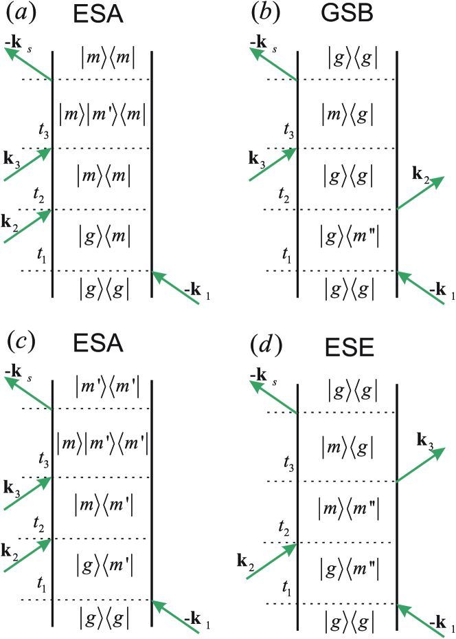
Figure 5: Feynman diagrams for the photon echo technique $\mathbf{k}_{s}=-\mathbf{k}_{1}+\mathbf{k}_{2}+\mathbf{k}_{3}$.

Even though the above two expression formally gives the nonlinear signal, it is hard to analyze. However it is convenient for numerical simulations due to expandability of the scattering matrix into the domain where the coulomb interaction may play its role. The detailed form of the scattering matrix which involves the Coulomb interaction is given in Ref.kavousanaki2009probing ; mukamel2007sum ; chernyak1998multidimensional . An alternative approach to derive the signal by using double-sided time ordered Keldish diagrams shown in Fig. 5. The diagrammatic approach (also known as ”sum over states”) can answer one of the fundamental question whether the nonzero scattering matrix is sufficient to calculate a nonlinear signal. The answer to that question is not trivial due to large number of interfering terms in Eqs. (75) and (103). The diagrams were constructed by blocking the consequent double excitation of the same electron-hole pair. The nonlinear signals can be extracted from the diagrams by the rules stated in Ref.mukamel2007sum ; abramavicius2009coherent . In our case the photon echo signal is obtained via the diagrams in Fig. 5:

$$S^{j1,j2,j3,j4}_{-\mathbf{k}_{1}+\mathbf{k}_{2}+\mathbf{k}_{3}}\left({\omega_{3}},\tau_{2},-\omega_{1}\right)$$ (76)

$$=\texttt{Re}\sum\limits_{m,m^{\prime}\neq m}\frac{\mu_{m}^{j1}}{-\omega_{1}-E_{m}}\frac{\mu^{\star,j2}_{m}\mu^{\star,j3}_{m^{\prime}}\mu^{j4}_{m}\texttt{e }^{-i\tau_{2}(E_{m}-E^{\star}_{m})}}{\omega_{3}-E_{m}-E_{m}^{\prime}+E_{m}}$$

$$+\frac{\mu_{m^{\prime}}^{j1}}{-\omega_{1}-E_{m^{\prime}}}\frac{\mu^{\star,j2}_{m^{\prime}}\mu^{\star,j3}_{m}\mu^{j4}_{m^{\prime}}\texttt{e }^{-i\tau_{2}(E_{m}-E^{\star}_{m^{\prime}})}}{\omega_{3}-E_{m}-E_{m}^{\prime}+E_{m}^{\prime}}$$

$$-\texttt{Re}\sum\limits_{m,m^{\prime\prime}}\frac{\mu_{m^{\prime\prime}}^{j1}}{-\omega_{1}+E_{m^{\prime\prime}}}[\frac{\mu^{\star,j2}_{m}\mu^{\star,j3}_{m^{\prime\prime}}\mu^{j4}_{m}}{\omega_{3}-E_{m}}$$

$$+\frac{\mu^{\star,j2}_{m^{\prime\prime}}\mu^{\star,j3}_{m}\mu^{j4}_{m^{\prime\prime}}\texttt{e}^{-i\tau_{2}\left({E_{m}-E^{\star}_{m^{\prime}}}\right)}}{\omega_{3}-E_{m}}]\ .$$

This signal would vanish if it were not for the Pauli blocking which prevents $m$ to be equal to $m^{\prime}$.

In Appendix D we have analyzed an alternative form of the four-wave mixing known as double-quantum coherence. This signal vanishes identically despite the Pauli induced scattering since the exited state absorption pathways are fully compensated by their ground state bleaching and exited state emission counterparts. Therefore the double-quantum-coherence can be readily used as a measure of the Coulomb interaction strength, and screening.

VI Numerical results and discussion

The main advantage of the Pauli blocking description of excitons is its simplicity. For a model with $N$ singly excited electronic states, we only need to consider $N$ double excited states compared with $N(N-1)$ in the case of Coulomb scattering induced biexcitons. We note that the same number of doubly excited states $N(N-1)$ are allowed in a simple boson harmonic model. This allows for better tracking of pathways interference and resonances. In this section, we shall use it to classify the off-diagonal resonances in the 2D photon echo spectra in accordance with the short living excited states of the QD. This will be compared with the linear absorption spectrum which is proportional to the single excited electronic density of states and is given by the main diagonal of the 2D spectra. We shall demonstrate the improved resolution of those short living states via the coherent response with the long living excitation. First, we assume the a model of two single excited states $(\mu-1,E_{1};\ \mu_{2},E_{2})$. This leads by the Pauli exclusion principle to the single double excited state $(\mu_{12},E_{1}+E_{2})$. The photon echo signal contains three distinct pathways: ground state bleaching (GSB Fig. 5(b)), excited state emission (ESE Fig. 5(d), and excited state absorption (ESA Fig. 5(a,c). Those are given by

$$S^{(3)}_{\texttt{GSB}}(\omega_{3},t_{2},\omega_{1})=\texttt{Re}\sum\limits_{i,j=1}^{2}\frac{|{\mu_{i}}|^{2}|{\mu_{j}}|^{2}}{\left({-\omega_{1}-E^{\star}_{i}}\right)\left({\omega_{3}-E_{j}}\right)}$$ (77)

$$S^{(3)}_{\texttt{ESE}}(\omega_{3},\tau_{2},\omega_{1})=\texttt{Re}\sum\limits_{i,j=1}^{2}\frac{|{\mu_{i}}|^{2}|{\mu_{j}}|^{2}\texttt{e}^{-\tau_{2}(E_{j}-E^{\star}_{i})}}{\left({-\omega_{1}-E^{\star}_{i}}\right)\left({\omega_{3}-E_{j}}\right)}$$ (78)

$$S^{(3)}_{\texttt{ESA}}(\omega_{3},\tau_{2},\omega_{1})$$ (79)

$$=-\texttt{Re}\sum\limits_{i\neq j}^{2}\frac{|{\mu_{i}}|^{2}|{\mu_{j}}|^{2}\texttt{e}^{-\tau_{2}(E_{i}-E^{\star}_{i})}}{\left({-\omega_{1}-E^{\star}_{i}}\right)\left({\omega_{3}-E_{j}-E_{i}+E^{\star}_{i}}\right)}$$

$$-\texttt{Re}\sum\limits_{i\neq j}^{2}\frac{|{\mu_{i}}|^{2}|{\mu_{j}}|^{2}\texttt{e}^{-\tau_{2}(E_{i}-E^{\star}_{j})}}{\left({-\omega_{1}-E^{\star}_{j}}\right)\left({\omega_{3}-E_{i}-E_{j}+E^{\star}_{j}}\right)}\ .$$

Clearly, when Pauli blocking is neglected, we have a collection of damped oscillators and at $\tau_{2}=0$ the signal disappears. It would also vanish if we assume that there is no damping in the system. We note that Pauli blocking may be suppressed when the double exciting state is formed by electron/hole pairs with opposite spins.

Since the nonlinear signal vanishes for ideal bosons, one can recast it to the alternative simplified form as if from the ESA from otherwise Pauli blocked $N$ states as

$$S^{(3)}_{-\mathbf{k}_{1}+\mathbf{k}_{2}+\mathbf{k}_{3}}\left({\omega_{3},0,-\omega_{1}}\right)$$ (80)

$$=2\texttt{Re}\sum\limits_{i=1}^{N}\frac{|{\mu_{i}}|^{2}|{\mu_{j}}|^{2}}{\left({-\omega_{1}-E^{\star}_{i}}\right)\left({\omega_{3}-E_{i}-E_{j}+E^{\star}_{j}}\right)}$$

At zero time delay $\tau_{2}=0$ we have only the diagonal resonances. The states with small damping dominate the picture. However as the time delay progresses the off diagonal resonances appear, as demonstrated in Fig. 6.

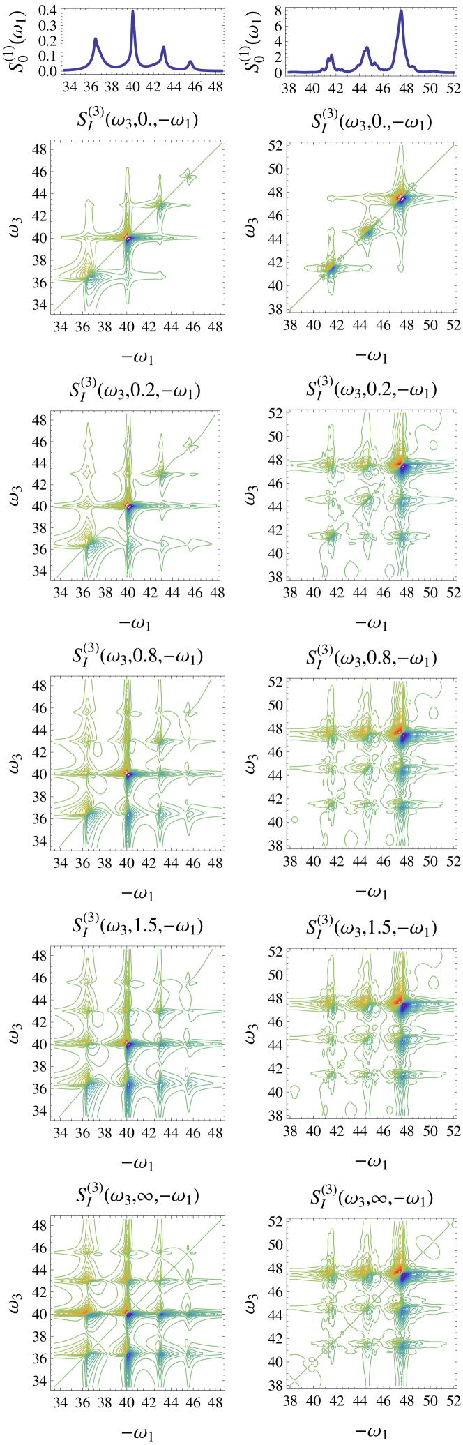
Figure 6: Photon echo signal for various time delays $\tau_{2}$ calculated from Eq. (76). The left panels correspond to $E_{g}=0$, while the right panels demonstrate the dressing effect $E_{g}=10$. The top-marginal graphs show the linear absorption.

It is convenient to interpret the signal by comparing it with the linear absorption (the top-marginal graph in the figure). For our numerical simulations, we chose the potential kink height to be $V_{1}=-V_{2}=20$. Unless stated otherwise, all the energies are in units of $3\tilde{\gamma}_{0}a/R$. We have also added constant dephasing rate $\gamma=0.1$ to account for possible contact with an external phonon bath. We have also limited ourselves to electronic states with angular momentum up to $m=9/2$. An idealized single graphene layer grown epitaxially on SiO was considered.

The tallest absorption peak comes from the transition $5/2\to 7/2$, and is located at $\omega_{1}\approx 40.0$. That signifies the true bound state when the electron (hole) energy reaches the height of the potential barrier (See Eq.  (59) and Fig. 3). The remaining absorption peaks correspond to quasi-bound states with finite lifetime. For the linear spectrum, the latter brings the peak broadening. To extract additional information about the dynamics of the quasi-bound states, we resort to the photon echo signal. At zero time delay $\tau_{2}=0$, this provides the same information as the linear absorption. The positions and magnitudes of the cross-peaks (rapid change in the sign of the signal) on the main diagonal correspond to those in the linear absorption. The existence of the signal comes from the fact that the electrons (holes) are not coupled to a simple bath of harmonic oscillators (constant dephasing). The pattern of the cross-resonances along the main diagonal is the manifestation of the destructive interference between the GSB, ESE on one side and the ESA pathways on the other. The latter takes into account the Pauli blocking effect on the biexciton (two electron-hole pair) states. At this point, we completely neglected the effect due to the Coulomb interaction between electrons. Later, we shall demonstrate that it is a reasonable assumption for small QDs. Thanks to the very simple exciton scattering matrix based on Pauli blocking, only (Eq. (74)), we can employ a simplified quasi-particle picture in order to describe the signal (Eq. (80)).

By increasing the time delay $\tau_{2}$, we may monitor the lifetime dynamics of the quasi-bound states as follows. The ESA and ESE contributions to the signal is reduced and finally the GSB signal survives (the lowest graphs in Fig. 6). In between, the off-diagonal cross-peaks appear at a time. Those with the smaller dephasing rate (strongly bound to the QD) appear first. The most pronounced cross-peaks are those which are correlated to the true bound state.

We next turn our attention to the dressed Dirac electrons confined to the potential induced QD. The dressing opens up a dynamical gap which can be controlled by the intensity and polarization degree of CW pumping light. We shall probe the dynamic gap by the photon echo technique described above and compare it to the linear absorption. The gap allows for many more bound states since the wave vector of the outgoing electronic wave $\kappa$ can cross over into the imaginary plane, thus effectively quenching the outgoing wave and bounding the electron states (See Fig. 3). For our simulations, we chose the gap $E_{g}=10$ which may be achieved either for small QD or intense pumping field with circular polarization. We note that the gap may also be induced by a polar substrateqaiumzadeh2009ground . The gap achieves several bound states for the $1/2\to 3/2$ electronic transitions. Since the wave functions for larger angular momentum are highly oscillatory, the latter transition posses highest oscillator strength, thereby effectively shifting the position of the main peak in the linear absorption (see Fig. 6 right panel). The remainder of the peaks also contain a mixture between the bound and quasi-bound states. To separate these, we shall look at the photon echo at $\tau_{2}>0$. Finally, the resulting GSB reveals the truly bound states (see Fig. 6 right panel).

To examine the role played by Coulomb scattering, we shall employ the full form of the scattering matrix. The approach is based on the nonlinear exciton equations (NEE). We refer the reader to the comprehensive review of the technique given by Abramavicus and Mukamel abramavicius2009coherent . Exciton scattering is best described in the eigenstate basis of Eqs. (58) and (53). Keeping in mind that we can have at most two excitons, leads to effective truncation schematics of otherwise infinite series of intertwined NEEsmukamel1995principles . In the latter case, an appropriate factorization scheme has been applied. We have also neglected incoherent exciton transport.

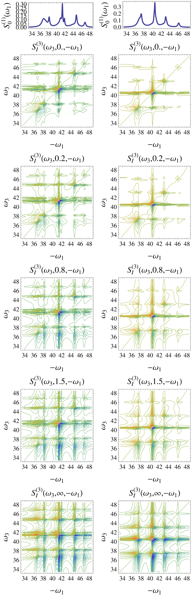
Figure 7: The same as in Fig. 6 with the Coulomb scattering taken into account via Eq. (75) with the scattering matrix given by Eq. The left panels represent large QD, $R/a_{0}=1000$. Right panels are for smaller QD, $R/a_{0}=100$.

The photon echo and the linear absorption are shown in the right panel of Fig. 7 for larger size QD. We see the off-diagonal correlation resonances and symmetry breaking for $\tau_{2}=0$. These indicates the bonding and anti-bonding biexciton resonances with the biexciton binding energy of a few eV. Indeed, when the biexciton binding energy is increased as a result of the Coulomb interaction, the ESA peaks are shifted along $\omega_{3}$: downwards for positive anti-binding (exciton repulsion) and upwards for negative bonding energy (exciton attraction). The ESA cross-peaks are no longer cancelled by the GSB and ESE, thus creating the doublets. By increasing the QD size, we see the formation of excitons with exciton binding energy of $10-30\;\texttt{eV}$ in the left panel of Fig. 7. Signatures of the off-diagonal quadratic coupling also persist for longer delay times $\tau_{2}>0$.

VII Concluding Remarks

We proposed dressing the Dirac electrons with circularly polarized photons in order to localize them within a QD on graphene monolayer. We also investigated the localization of dressed electrons in a cylindrical QD formed on bilayer graphene. When graphene is irradiated with a circularly polarized electromagnetic field, An energy gap opens up in the dispersion relation for graphene in the presence of this electromagnetic field. Consequently, the resulting confined electronic states for a QD seem to have properties that are similar in nature to the surface states of topological insulators. Their energies are located inside the energy gap and the wave functions decay as a function of distance from the interface of the potential. These topological states are robust with respect to the effects of disorder. Our calculations showed that the dressing does not only open a dynamical gap in the energy dispersion spectrum, but it also leads to a renormalization of the Fermi velocity as well as the intra layer and inter layer coupling parameters. In fact, in the bilayer configuration, the dressing serves as a tool for tuning the energy gap. That is, it can either close or open the gap, depending on the polarity of the potential and the direction of the light polarization. Linear spectroscopy cannot resolve the short lived broadened excitonic states and must be resolved by using a four-wave mixing technique known as photon-echo. This eliminates the inhomogeneous broadening due to impurities, and to focuses on the intrinsic lifetimes of the electronic states. We measure the localization through the electronic density of states, The strong dynamical screening of the Coulomb interaction leads us to consider only the Pauli blocking due to the Fermi statistics. We simplify the signal interpretation by switching to the quasiparticle picture. Those are give as the deviation from the harmonic oscillator for which the nonlinear signals disappear. This allows us to consider only excited states absorption Liouville pathways. In this way, we are able to reduce the interference due to the usual combination between the ground state bleaching and excited states emission. Visible light is used to map the QD interband transitions onto 2D spectra and terahertz pulse shaped fields for the intraband transitions. Important aspects of terahertz pulse shaped fields for the intraband transitions will be reported elsewhere. The latter will allow us to use a novel and more convenient phase cycling method to obtain the $\chi^{(3)}$ response kuehn2011strong .

Appendix A Derivation of Eq. (1)

The original Hamiltonian has the form

$$\mathcal{H}=\hbar v_{F}\bm{\sigma}\cdot\left({\mathbf{k}-\frac{e}{c\hbar}\mathbf{A}}\right)$$ (81)

The vector potential operator of the electromagnetic field can be partitioned as:

$$\mathbf{A}=\mathbf{A}_{0}+\sum\limits_{i=1}^{\infty}\mathbf{A}_{i}$$ (82)

$$\mathbf{A}_{0}=\sqrt{\frac{2\pi\hbar c^{2}}{\omega_{0}\Omega}}\left({\mathbf{e}_{+}a_{0}+\mathbf{e}_{-}a^{\dagger}_{0}}\right)$$ (83)

$$\mathbf{A}_{i}=\sqrt{\frac{2\pi\hbar c^{2}}{\omega_{i}\Omega}}\left({\mathbf{e}_{x}(a_{i}+a^{\dagger}_{i})}\right)$$ (84)

Here $\sqrt{2}\mathbf{e}_{\pm}=\mathbf{e}_{x}\pm i\mathbf{e}_{y}$ are polarization vectors given in terms of the unit vectors along corresponding Cartesian directions; $\Omega$ is the mode quantization volume. As one can see Eq. (82) describes the electromagnetic wave propagating along $z-$axis (transverse to graphene). It is clock-wise circularly polarized. We will need the circular polarization since graphene is gapless and no RWA is applicable. The rest of the optical modes described by Eq. (83) are linearly polarized. Note that we have no phase on the optical filed since we assume graphene being ideally flat and situated at $z=0$. That is $\exp(\pm ik_{z}z)=1$. Substituting Eq. (82) into Eq. (81) and denoting $-e\sqrt{4\pi\hbar v^{2}_{F}/\omega_{i}\Omega}=W_{i}/\sqrt{N_{i}}$ in order to keep notation consistent with Ref. gerry2003introduction we obtain Eq. (1).

Appendix B Derivation of Eqs. (18) and (19)

We first need the following identities

$$\sigma_{\pm}|{\pm,N_{0}}\rangle=|{\mp,N_{0}}\rangle$$ (85)

$$\sigma_{\pm}|{\mp,N_{0}}\rangle=0$$ (86)

Therefore, we shall have:

$$\hbar v_{F}\left({\sigma_{x}k_{x}+\sigma_{y}k_{y}}\right)|{\psi_{\pm,N_{0}}}\rangle$$ (87)

$$=\hbar v_{F}\left({(\sigma_{+}+\sigma_{-})k_{x}+i(\sigma_{-}-\sigma_{+})k_{y}}\right)|{\psi_{\pm,N_{0}}}\rangle$$

$$=\hbar v_{F}\left({(\sigma_{+}+\sigma_{-})k_{x}+i(\sigma_{-}-\sigma_{+})k_{y}}\right)$$

$$\times\left({\cos\phi|{\pm,N_{0}}\rangle\pm\sin\phi|{\mp,N_{0}\pm 1}\rangle}\right)$$

$$=\hbar v_{F}(k_{x}\left({\cos\phi|{\mp,N_{0}}\rangle\pm\sin\phi|{\pm,N_{0}\pm 1}\rangle}\right)\pm$$

$$\pm ik_{y}\left({\cos\phi|{\mp,N_{0}}\rangle\mp\sin\phi|{\pm,N_{0}\pm 1}\rangle}\right))$$

Using the above equation we can calculate all the necessary matrix elements:

$$\mathcal{H}_{1}=\tilde{\mathcal{H}}_{1}+V(x,y)$$

$$\langle{\psi_{+,N_{0}}}|\tilde{\mathcal{H}}_{1}|{\psi_{+,N_{0}}}\rangle$$ (88)

$$=\hbar v_{F}((\cos\phi Phys.~{}Lett.~{}{N_{0}}+\sin\phi\langle{-,N_{0}+1}|)$$

$$\times k_{x}\left({\cos\phi|{-,N_{0}}\rangle+\sin\phi|{+,N_{0}+1}\rangle}\right)$$

$$+ik_{y}\left({\cos\phi|{-,N_{0}}\rangle-\sin\phi|{+,N_{0}+1}\rangle}\right))=0$$

$$\langle{\psi_{-,N_{0}}}|\tilde{\mathcal{H}}_{1}|{\psi_{-,N_{0}}}\rangle$$ (89)

$$=\hbar v_{F}((\cos\phi\langle{-,N_{0}}|-\sin\phi Phys.~{}Lett.~{}{N_{0}-1})$$

$$\times k_{x}\left({\cos\phi|{+,N_{0}}\rangle-\sin\phi|{-,N_{0}-1}\rangle}\right)$$

$$-ik_{y}\left({\cos\phi|{+,N_{0}}\rangle+\sin\phi|{-,N_{0}-1}\rangle}\right))=0$$

$$\langle{\psi_{-,N_{0}}}|\tilde{\mathcal{H}}_{1}|{\psi_{+,N_{0}}}\rangle$$

$$=\hbar v_{F}((\cos\phi\langle{-,N_{0}}|-\sin\phi Phys.~{}Lett.~{}{N_{0}-1})$$

$$\times k_{x}\left({\cos\phi|{-,N_{0}}\rangle+\sin\phi|{+,N_{0}+1}\rangle}\right)$$

$$+ik_{y}\left({\cos\phi|{-,N_{0}}\rangle-\sin\phi|{+,N_{0}+1}\rangle}\right))$$

$$=\cos^{2}\phi\left({k_{x}+ik_{y}}\right)$$

$$\langle{\psi_{+,N_{0}}}|\tilde{\mathcal{H}}_{1}|{\psi_{-,N_{0}}}\rangle$$ (91)

$$=\hbar v_{F}((\cos\phi Phys.~{}Lett.~{}{N_{0}}+\sin\phi\langle{-,N_{0}+1}|)$$

$$\times k_{x}\left({\cos\phi|{+,N_{0}}\rangle-\sin\phi|{-,N_{0}-1}\rangle}\right)$$

$$-ik_{y}\left({\cos\phi|{+,N_{0}}\rangle+\sin\phi|{-,N_{0}-1}\rangle}\right))$$

$$=\cos^{2}\phi\left({k_{x}-ik_{y}}\right)$$

$$\langle{\psi_{\pm,N_{0}}}|V(x,y)|{\psi_{\pm,N_{0}}}\rangle$$ (92)

$$=V(x,y)\left({\cos^{2}\phi+\sin^{2}\phi}\right)=V(x,y)$$

For $\mathcal{H}_{2}$ matrix elements we will need, the following identities.

$$\langle{\psi_{\pm,N_{0}}}|\sigma_{+}+\sigma_{-}|{\psi_{\pm,N_{0}}}\rangle$$ (93)

$$=\langle{\psi_{\pm,N_{0}}}|\left({\cos\phi|{\mp,N_{0}}\rangle\pm\sin\phi|{\pm,N_{0}\pm 1}\rangle}\right)$$

$$=\left({\cos\phi\langle{\pm,N_{0}}|\pm\sin\phi\langle{\mp,N_{0}\pm 1}|}\right)$$

$$\times\left({\cos\phi|{\mp,N_{0}}\rangle\pm\sin\phi|{\pm,N_{0}\pm 1}\rangle}\right)=0$$

$$\langle{\psi_{\mp,N_{0}}}|\sigma_{+}+\sigma_{-}|{\psi_{\pm,N_{0}}}\rangle=\cos^{2}\phi$$ (94)

Appendix C Derivation of Eqs. (33) and (34)

For the b-layer we will need the following identities:

$$\langle{\psi_{N_{0}}}|\sigma_{\pm}|{\psi_{N_{0}}}\rangle$$ (95)

$$=\left({\begin{array}[]{cc}\langle{\psi_{+,N_{0}}}|\sigma_{\pm}|{\psi_{+,N_{0}}}\rangle&\langle{\psi_{+,N_{0}}}|\sigma_{\pm}|{\psi_{-,N_{0}}}\rangle\\ \langle{\psi_{-,N_{0}}}|\sigma_{\pm}|{\psi_{+,N_{0}}}\rangle&\langle{\psi_{-,N_{0}}}|\sigma_{\pm}|{\psi_{-,N_{0}}}\rangle\end{array}}\right)$$ (98)

$$=\left({\cos^{2}\phi}\right)\sigma_{\pm}$$

$$\langle{\psi_{N_{0}}}|\sigma_{+}a_{0}|{\psi_{N_{0}}}\rangle=\langle{\psi_{N_{0}}}|\sigma_{-}a^{\dagger}_{0}|{\psi_{N_{0}}}\rangle$$ (99)

$$=\frac{\sqrt{N_{0}}}{2}\sin 2\phi\left({\begin{array}[]{cc}1&0\\ 0&-1\end{array}}\right)=\left({\frac{\sqrt{N_{0}}}{2}\sin 2\phi}\right)\sigma_{3}$$ (102)

Appendix D Double quantum coherence.

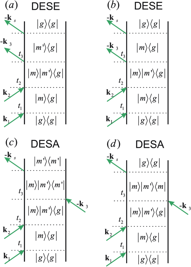
Figure 8: Feynman diagrams for the double quantum coherence signal generated in $\mathbf{k}_{s}=\mathbf{k}_{1}+\mathbf{k}_{2}-\mathbf{k}_{3}$ direction.

The double quantum coherence signal can be derived from the diagrams in Fig. 8 assuming the following form:

$$S^{j1,j2,j3,j4}_{\mathbf{k}_{1}+\mathbf{k}_{2}-\mathbf{k}_{3}}\left({\omega_{3}},\omega_{2},\tau_{1}=0\right)$$ (103)

$$=2\texttt{Im}\sum\limits_{e1,e2,e3,e4}\mu^{\star,j1}_{e1}\mu^{\star,j2}_{e2}\mu^{j3}_{e3}\mu^{j4}_{e4}G_{e4}(\omega_{3})G^{\star}_{e3}(\omega_{2}-\omega_{3})$$

$$\times\left[{\Gamma_{e4,e3;e2,e1}(\omega_{3}+E_{e3})G_{e2,e1}(\omega_{3}+E_{e1})-}\right.$$

$$\left.{-\Gamma_{e4,e3;e2,e1}(\omega_{2})G_{e2,e1}(\omega_{2})}\right]$$

When the Coulomb scattering may be neglected the above signal is greatly simplified into sum-over-states expression with the explicit Pauli blocking principle:

$$S^{j1,j2,j3,j4}_{\mathbf{k}_{1}+\mathbf{k}_{2}-\mathbf{k}_{3}}\left({\omega_{3}},\omega_{2},\tau_{1}\right)$$ (104)

$$=\texttt{Re}\sum\limits_{m,m^{\prime}\neq m}\frac{\mu^{\star,j1}_{m}\mu^{\star,j2}_{m^{\prime}}\texttt{e}^{-iE_{m}\tau_{1}}}{\omega_{2}-E_{m}-E_{m^{\prime}}}$$

$$\times\left[{\frac{\mu^{j3}_{m}\mu^{j4}_{m^{\prime}}}{\omega_{3}-E_{m}-E_{m^{\prime}}+E_{m^{\prime}}}+\frac{\mu^{j3}_{m^{\prime}}\mu^{j4}_{m}}{\omega_{3}-E_{m}-E_{m^{\prime}}+E_{m}}-}\right.$$

$$\left.{-\frac{\mu^{j3}_{m^{\prime}}\mu^{j4}_{m}}{\omega_{3}-E_{m}-E_{m^{\prime}}+E_{m^{\prime}}}-\frac{\mu^{j3}_{m}\mu^{j4}_{m^{\prime}}}{\omega_{3}-E_{m}-E_{m^{\prime}}+E_{m}}}\right]$$

This signal vanishes identically despite the Pauli induced scattering making it a measure of the screened Coulomb interaction.

References

• (1) A. H. Castro Neto, F. Guinea, N. M. R. Peres, K. S. Novoselov, and A. K. Geim, “The electronic properties of graphene,” Reviews of modern physics 81, 109–162 (2009).
• (2) L. J. P. Xavier, J. M. Pereira, A. Chaves, G. A. Farias, and F. M. Peeters, “Topological confinement in graphene bilayer quantum rings,” Applied Physics Letters 96, 212108 (2010).
• (3) T. Paananen, R. Egger, and H. Siedentop, “Signatures of wigner molecule formation in interacting dirac fermion quantum dots,” Physical Review B 83, 085409 (2011).
• (4) G. Pal, W. Apel, and L. Schweitzer, “Electric transport through circular graphene quantum dots: presence of disorder,” Arxiv preprint arXiv:1107.0113(2011).
• (5) C. H. Park and S. G. Louie, “Tunable excitons in biased bilayer graphene,” Nano letters 10, 426–431 (2010).
• (6) A. Matulis and F. M. Peeters, “Quasibound states of quantum dots in single and bilayer graphene,” Physical Review B 77, 115423 (2008).
• (7) B. Wunsch, T. Stauber, and F. Guinea, “Electron-electron interactions and charging effects in graphene quantum dots,” Physical Review B 77, 035316 (2008).
• (8) P. Hewageegana and V. Apalkov, “Electron localization in graphene quantum dots,” Physical Review B 77, 245426 (2008).
• (9) O. V. Kibis, “Metal-insulator transition in graphene induced by circularly polarized photons,” Physical Review B 81, 165433 (2010).
• (10) Y. Zhou and M. W. Wu, “Optical response of graphene under intense terahertz fields,” Physical Review B 83, 245436 (2011).
• (11) D. Abramavicius, B. Palmieri, D.V. Voronine, F. Šanda, and S. Mukamel, “Coherent multidimensional optical spectroscopy of excitons in molecular aggregates; quasiparticle versus supermolecule perspectives,” Chemical reviews 109, 2350–2408 (2009).
• (12) W. Kuehn, K. Reimann, M. Woerner, T. Elsaesser, R. Hey, and U. Schade, “Strong correlation of electronic and lattice excitations in gaas/algaas semiconductor quantum wells revealed by two-dimensional terahertz spectroscopy,” Physical Review Letters 107, 67401 (2011).
• (13) E. G. Kavousanaki, O. Roslyak, and S. Mukamel, “Probing excitons and biexcitons in coupled quantum dots by coherent two-dimensional optical spectroscopy,” Physical Review B 79, 155324 (2009).
• (14) C. Gerry and P. Knight, Introductory Quantum Optics (Cambridge Univercity Press, 2003).
• (15) S. Mukamel, Principles of Nonlinear Optics and Spectroscopy (Oxford University Press, 1995).
• (16) S. Mukamel, R. Oszwaldowski, and D. Abramavicius, “Sum-over-states versus quasiparticle pictures of coherent correlation spectroscopy of excitons in semiconductors: Femtosecond analogs of multidimensional nmr,” Physical Review B 75, 245305 (2007).
• (17) V. Chernyak, W. M. Zhang, and S. Mukamel, “Multidimensional femtosecond spectroscopies of molecular aggregates and semiconductor nanostructures: The nonlinear exciton equations,” The Journal of chemical physics 109, 9587 (1998).
• (18) The interaction is modified by the dressing, as indicated by tilde.
• (19) V. M. Agranovich, “Electrodynamics of excitons in two-dimensional systems,”  (Taylor & Francis, 1992).
• (20) A. Qaiumzadeh and R. Asgari, “Ground-state properties of gapped graphene using the random phase approximation,” Physical Review B 79, 075414 (2009).