Superfluid pairing in a mixture of a spin-polarized Fermi gas and a dipolar condensate

Abstract

We consider a mixture of a spin-polarized Fermi gas and a dipolar Bose-Einstein condensate in which s-wave scattering between fermions and the quasiparticles of the dipolar condensate can result in an effective attractive Fermi-Fermi interaction anisotropic in nature and tunable by the dipolar interaction.  We show that such an interaction can significantly increase the prospect of realizing a superfluid with a gap parameter characterized with a coherent superposition of all odd partial waves. We formulate, in the spirit of the Hartree-Fock-Bogoliubov mean-field approach, a theory which allows us to estimate the critical temperature when the anisotropic Fock potential is taken into consideration and to determine the system parameters that optimize the critical temperature at which such a superfluid emerges before the system begins to phase separate.

I Introduction

Superfluid pairing of fermions in the $l$th partial wave depends on the two-body scattering amplitude $f_{l}$.  According to Wigner’s threshold laws landau89 , $f_{l}$ scales as $\left(k_{F}^{0}\right)^{2l}$ for typical ground state atoms, where $\hbar k_{F}^{0}$ is the Fermi momentum. This reduces the critical temperature for the p-wave ($l=1$) Bardee-Cooper-Schrieffer (BCS) superfluid to such a low level that it is virtually inaccessible to current technology, except in situations where Wigner’s threshold laws are not respected.  A case in point is tuning atoms near the p-wave Feshbach resonance bohn00 ; klinkhamer04 ; ohashi05 ; ho05 , where p-wave scattering can be dramatically enhanced.  This excited the hope of realizing $p$-wave superfluids via p-wave Feshbach resonances in the ultracold atomic physics community. But, due to an increased number of inelastic collisions near the resonance, “Feshbach molecules” are short lived regal03 ; zhang04 ; ticknor04 ; gunter05 , and such a prospect appears difficult to attain.  Another example, first pointed out by You and Marinescu marinescu98 , is subjecting a dipolar Fermi gas to a sufficiently strong DC electric field, where p-wave scattering can also be enhanced.  A subsequent detailed investigation by Baranov et al. baranov02 indicates that the order parameter in such a spin-polarized dipolar Fermi gas is unusual in the sense that it is the superposition of all odd partial waves.  Recently there has been an upsurge of effort aimed at achieving unusual Fermi pairings in both two-component and single component dipolar Fermi gases samokhin06 ; bruun08 ; wu10 ; shi10 ; liao10 ; ronen10 ; zhao10 along the direction of You and Marinescu marinescu98 ,  motivated largely by recent rapid experimental advancement in achieving ultracold dense dipolar gases in ⁴⁰K -⁸⁷Rb polar molecules ospelkaus08 ; ni08 ; ospelkaus09 and in Cr stuhler05 , spin-1 Rb vengalattore08 , and Dy lu11 atoms.

In the present work, we focus on an alternative route towards the same goal, seeking to engineer unusual superfluid pairings in mixtures of different degenerate quantum gases. Cold-atom systems, besides being capable of unprecedented controllability (interaction strength, dimensionality, etc.), enjoy the distinct advantage over traditional solid-state systems of being easily mixed to form new states of quantum gases and liquids.  Bose-Bose, Bose-Fermi, and Fermi-Fermi mixtures of different isotopes or species are now readily accessible under (sophisticated) laboratory conditions (see shin08 ; park11 ; wu11 and references therein). As is well known, due to the density fluctuation of Bose condensates, mixing bosons can induce an effective attraction between two fermions bijlsma00 .  This was the mechanism in Efremov and Viverit’s proposal efremov02 to achieve p-wave Cooper pairings in a single-component Fermi-Bose mixture.  A generalization of the scheme to a two-dimensional (2D) mixture involving dipolar bosons was recently carried out by Dutta and Lewenstein dutta10 , with the goal of realizing a superfluid with $p_{x}+ip_{y}$ symmetry whose excitations are non-Abelian anyons that are the building blocks for topological quantum computation nayak08 .  Nishida nishida09 and Nishida and Tan nishida10 sought to achieve the same goal by inducing p-wave and higher partial-wave resonances from s-wave Feshbach resonance between atoms from different Fermi gases in different dimensions. In a recent article kain11 , we explored singlet and triplet superfluid competition in a mixture of two-component Fermi and one-component dipolar Bose gases.

In this paper, we consider a three-dimensional (3D) mixture between (nondipolar) fermions of mass $m_{F}$ in ground state $\left|a\right\rangle$ and (dipolar) bosons of mass $m_{B}$ in ground state $\left|b\right\rangle$, with their dipoles oriented along the $z$ direction established by an external (either electric or magnetic) field.  In contrast to the phonon spectrum of a nondiploar condensate, which is isotropic, the phonon spectrum of a dipolar condensate is anisotropic goral00 ; giovanazzi02 .  Such anisotropic phonons will thus induce an anisotropic Fermi-Fermi interaction, thereby providing an alternative mechanism for creating a superfluid (in the mixture between a spin polarized Fermi gas and a dipolar condensate) with an order parameter which is the superposition of all odd partial waves.

The outline of our paper is as follows.  In Sec. II, we develop, within the framework of the Hartree-Fock-Bogoliubov mean-field approach, a theoretical foundation for self-consistently addressing challenges we will face in later sections.  These challenges include the anisotropy of the induced interaction and the limitations due to phase separation.  In Sec. III, we calculate the critical temperature taking into consideration the anisotropic Fock potential with the help of the variational method, and we show that properly tuning the dipolar interaction can dramatically increase the critical temperature in the long wavelength limit.   In Sec. IV, we review the subject of phase separation and develop a procedure that allows us to determine the system parameters for achieving the optimal critical temperature before the system begins to phase separate.  We summarize and conclude in Sec. V.

II Theoretical Formulation

II.1 Bare Model

In our model the low temperature physics arises from the interplay between short- and long-range two-body interactions.  The short-range interaction is dominated by s-wave collisions which, given that the Pauli exclusion principle forbids such interactions taking place between two identical fermions, are parameterized with two scattering lengths, $a_{BB}$ and $a_{BF}$, characterizing s-wave scattering between two bosons and between a boson and a fermion, respectively.  The long-range interaction is the dipole-dipole interaction (restricted only to bosons in our model), which varies with $\mathbf{r}$, the separation between two particles in position space, according to $U_{DD}\left(\mathbf{r}\right)=d^{2}\left(1-3z^{2}/r^{2}\right)/r^{3}$, where $d^{2}$ represents the dipolar interaction strength.   Assuming that the mixture is sufficiently large so that it can be treated as a uniform system with an effective volume $V$, we model such a mixture with a (grand canonical) Hamiltonian $\hat{H}=\hat{H}_{B}+\hat{H}_{F}+\hat{H}_{BF}$ in momentum space according to

$$\hat{H}_{B} =\sum_{\mathbf{k}}\left(\epsilon_{\mathbf{k},B}-u_{B}\right)\hat{b}_{\mathbf{k}}^{{\dagger}}\hat{b}_{\mathbf{k}}+\left(2V\right)^{-1}\times$$

$$\sum_{\mathbf{k},\mathbf{k}^{\prime},\mathbf{q}}\left[U_{BB}+U_{DD}\left(\mathbf{q}\right)\right]\hat{b}_{\mathbf{k}+\mathbf{q}}^{{\dagger}}\hat{b}_{\mathbf{k}^{\prime}-\mathbf{q}}^{{\dagger}}\hat{b}_{\mathbf{k}^{\prime}}\hat{b}_{\mathbf{k}},$$ (1)

$$\hat{H}_{F} =\sum_{\mathbf{k},\sigma}\left(\epsilon_{\mathbf{k},F}-u_{F}\right)\hat{a}_{\mathbf{k}}^{{\dagger}}\hat{a}_{\mathbf{k}},$$ (2)

$$\hat{H}_{BF} =U_{BF}V^{-1}\sum_{\mathbf{k},\mathbf{k}^{\prime},\mathbf{q}}\hat{a}_{\mathbf{k}}^{{\dagger}}\hat{a}_{\mathbf{k}+\mathbf{q}}\hat{b}_{\mathbf{k}^{\prime}}^{{\dagger}}\hat{b}_{\mathbf{k}^{\prime}-\mathbf{q}},$$ (3)

where $\hat{b}_{\mathbf{k}}$ ($\hat{a}_{\mathbf{k}}$) is the field operator for annihilating a boson (a fermion) with kinetic energy $\epsilon_{\mathbf{k},B}=\hbar^{2}k^{2}/2m_{B}$ $\left(\epsilon_{\mathbf{k},F}=\hbar^{2}k^{2}/2m_{F}\right)$ and chemical potential $u_{B}$ ($u_{F}$); $U_{BB}=4\pi\hbar^{2}a_{BB}/m_{B}$ and $U_{BF}=4\pi\hbar^{2}a_{BF}/m_{BF}$ with $m_{BF}=2m_{B}m_{F}/(m_{B}+m_{F})$ measure the related s-wave scattering strengths; $U_{DD}\left(\mathbf{k}\right)=8\pi d^{2}P_{2}\left(\cos\theta_{\mathbf{k}}\right)/3$ is the dipole-dipole interaction in momentum space, with $P_{2}\left(x\right)=\left(3x^{2}-1\right)/2$ the second-order Legendre polynomial and $\theta_{\mathbf{k}}$ ($\phi_{\mathbf{k}}$) the polar (azimuthal) angle of vector $\mathbf{k}$.

II.2 Effective (or Dressed) Model

We consider the low temperature regime where virtually all bosons are condensed to the zero-momentum mode so that we can apply the usual Bogoliubov ansatz, in which $\hat{b}_{\mathbf{k}=0}$ is treated as a c-number $b_{\mathbf{k}=0}$.  This transforms Eq. (1) into a diagonalized form with the familiar interpretation that the bosonic system described by Eq. (1) is equivalent to a homogeneous dipolar condensate with density $n_{B}=\left|b_{\mathbf{k}=0}\right|^{2}$ plus a collection of phonon modes that obey the Bogoliubov dispersion relation goral00 ; giovanazzi02

$$E_{\mathbf{k}}=v_{B}\hbar k\sqrt{1+\left(\xi_{B}k\right)^{2}+2\varepsilon_{dd}P_{2}\left(\cos\theta_{\mathbf{k}}\right)},$$ (4)

where $\varepsilon_{dd}=4\pi d^{2}/(3U_{BB})$ dell04 measures the dipolar interaction relative to the s-wave collision, $v_{B}=\sqrt{n_{B}U_{BB}/m_{B}}$ is the phonon speed, and $\xi_{B}$ $=\hbar/\sqrt{4m_{B}n_{B}U_{BB}}$ is the healing length.  As can be seen, when $\varepsilon_{dd}$ $>$ $1$, phonons with $k\rightarrow 0$ acquire imaginary frequencies. In our study, then, we will limit $\ \varepsilon_{dd}$  to be less than one so that the dipolar condensate is stable against collapse.  Integrating out the phonon degrees of freedom as in Ref. bijlsma00 leads to an effective Bose-Fermi model described by the Hamiltonian

$$\hat{H}^{E}=H_{B}^{0}+\hat{H}_{F}^{E},$$ (5)

where

$$H_{B}^{0}=V\left(\frac{1}{2}U_{BB}n_{B}^{2}-u_{B}n_{B}\right)$$ (6)

accounts for the condensate energy, and

$$\hat{H}_{F}^{E} =\sum_{\mathbf{k}}\left(\epsilon_{\mathbf{k},F}-u_{F}+U_{BF}n_{B}\right)\hat{a}_{\mathbf{k}}^{{\dagger}}\hat{a}_{\mathbf{k}}+$$

$$\frac{1}{2V}\sum_{\mathbf{k},\mathbf{k}^{\prime},\mathbf{q}}U\left(\mathbf{q}\right)\hat{a}_{\mathbf{k}+\mathbf{q}}^{{\dagger}}\hat{a}_{\mathbf{k}^{\prime}-\mathbf{q}}^{{\dagger}}\hat{a}_{\mathbf{k}^{\prime}}\hat{a}_{\mathbf{k}},$$ (7)

is the effective Hamiltonian for the dressed fermions. In Eq. (7),

$$U\left(\mathbf{k}\right)=\frac{U\left(0\right)}{1+\left(\xi_{B}k\right)^{2}+2\varepsilon_{dd}P_{2}\left(\cos\theta_{\mathbf{k}}\right)}$$ (8)

is the phonon-induced Fermi-Fermi interaction in the static limit bijlsma00 ; efremov02 . It is well known that the dipolar interaction in position space is zero when averaged over all directions or, equivalently, the dipolar interaction in momentum space, $U_{DD}\left(\mathbf{k}\right)$, satisfies $U_{DD}\left(\mathbf{k}=0\right)=0$ and thus $U_{DD}\left(\mathbf{k}\right)$ is non analytic when $\mathbf{k}$ approaches zero chan10 .  For the same reason, the induced interaction $U\left(\mathbf{k}\right)$ is also non analytic when $\mathbf{k}$ approaches zero, but instead of being zero, $U\left(\mathbf{k}=0\right)$ approaches the finite value

$$U\left(0\right)=-U_{BF}^{2}/U_{BB}\text{,}$$ (9)

which is certainly different from $U\left(\mathbf{k}\rightarrow 0\right)$ according to Eq. (8) due to its dependence on the polar angle in the denominator.  As can be seen, the induced interaction depends on the dipole orientation differently than the direct dipole-dipole interaction and therefore provides an alternative mechanism for the exploration of the physics behind the anisotropy-related unusual Fermi pairings.

II.3 Hartree-Fock-Bogoliubov Mean-Field Theoretical Treatment

To study the superfluidity of a fermionic system described by the effective Hamiltonian (7), we use the self-consistent Hartree-Fock mean-field approach gennes89 in which we pair fermionic field operators in the two-body interaction part of the Hamiltonian in Eq. (7) according to Wick’s theorem, associating direct pairing with the Hartree potential

$$\Sigma^{{}^{\prime}}=U\left(0\right)n_{F}\text{,}$$ (10)

exchange pairing with the Fock potential

$$\Sigma\left(\mathbf{k}\right)=-\frac{1}{V}\sum_{\mathbf{k}^{\prime}}U\left(\mathbf{k}-\mathbf{k}^{\prime}\right)\left\langle\hat{a}_{\mathbf{k}^{\prime}}^{{\dagger}}\hat{a}_{\mathbf{k}^{\prime}}\right\rangle,$$ (11)

and BCS pairing with the gap parameter between fermionic pairs of opposite momenta

$$\Delta\left(\mathbf{k}\right)=\frac{1}{V}\sum_{\mathbf{k}^{\prime}}U_{A}\left(\mathbf{k},\mathbf{k}^{\prime}\right)\left\langle\hat{a}_{-\mathbf{k}^{\prime}}\hat{a}_{\mathbf{k}^{\prime}}\right\rangle,$$ (12)

where $n_{F}$ is the Fermi number density.  In arriving at Eq. (12), we used a symmetrized induced interaction

$$U_{A}\left(\mathbf{k},\mathbf{k}^{\prime}\right)=\frac{1}{2}\left[U\left(\mathbf{k}-\mathbf{k}^{\prime}\right)-U\left(\mathbf{k}+\mathbf{k}^{\prime}\right)\right],$$ (13)

in order to explicitly restrict the gap parameter to the sector in which $\Delta\left(\mathbf{k}\right)=-\Delta\left(-\mathbf{k}\right)$, a constraint imposed by Fermi statistics (or equivalently the Pauli exclusion principle).  This means that $\Delta\left(\mathbf{k}\right)$ will be a superposition involving all odd partial waves when the Fermi-Fermi interaction is anisotropic kain11 , as is the case with our model here .

The effective Hamiltonian in Eq. (5) now becomes the mean-field Hamiltonian

$$\hat{H}^{M}=H_{B}^{0}+H_{F}^{0}+\hat{H}_{F}^{{}^{M}},$$ (14)

where $H_{B}^{0}$ has already been defined in Eq. (6), and the other two are defined, in terms of the self-consistent mean fields introduced in Eqs. (10) - (12), as

$$\hat{H}_{F}^{M} =\sum_{\mathbf{k}}\left[\xi_{\mathbf{k}}=\epsilon_{\mathbf{k},F}-\mu_{F}+\Sigma\left(\mathbf{k}\right)\right]\hat{a}_{\mathbf{k}}^{{\dagger}}\hat{a}_{\mathbf{k}}$$

$$+ \frac{1}{2}\sum_{\mathbf{k}}\left[\Delta\left(\mathbf{k}\right)\hat{a}_{\mathbf{k}}^{{\dagger}}\hat{a}_{-\mathbf{k}}^{{\dagger}}+h.c\right],$$ (15)

where $\mu_{F}$ is an effective chemical potential for fermions defined by

$$\mu_{F}=u_{F}-\left[U\left(0\right)n_{F}+U_{BF}n_{B}\right],$$ (16)

and

$$H_{F}^{0}=-V\frac{1}{2}U\left(0\right)n_{F}^{2}$$

$$-\frac{1}{2}\sum_{\mathbf{k}}\Sigma\left(\mathbf{k}\right)\left\langle\hat{a}_{\mathbf{k}}^{{\dagger}}\hat{a}_{\mathbf{k}}\right\rangle-\frac{1}{2}\sum_{\mathbf{k}}\Delta\left(\mathbf{k}\right)\left\langle\hat{a}_{\mathbf{k}}^{{\dagger}}\hat{a}_{-\mathbf{k}}^{{\dagger}}\right\rangle,$$ (17)

or equivalently

$$H_{F}^{0} =-V\frac{1}{2}U\left(0\right)n_{F}^{2}$$

$$+\frac{1}{2}\sum_{\mathbf{k},\mathbf{k}^{\prime}}\Sigma\left(\mathbf{k}\right)U^{-1}\left(\mathbf{k}-\mathbf{k}^{\prime}\right)\Sigma\left(\mathbf{k}^{\prime}\right)$$

$$-\frac{1}{2}\sum_{\mathbf{k},\mathbf{k}^{\prime}}\Delta\left(\mathbf{k}\right)U_{A}^{-1}\left(\mathbf{k},\mathbf{k}^{\prime}\right)\Delta^{\ast}\left(\mathbf{k}^{\prime}\right),$$ (18)

where the inverse matrices are defined as $V^{-1}\sum_{\mathbf{k}^{\prime\prime}}U\left(\mathbf{k}-\mathbf{k}^{\prime\prime}\right)U^{-1}\left(\mathbf{k}^{\prime\prime}-\mathbf{k}^{\prime}\right)=\delta_{\mathbf{k},\mathbf{k}^{\prime}}$ and $V^{-1}\sum_{\mathbf{k}^{\prime\prime}}U_{A}\left(\mathbf{k},\mathbf{k}^{\prime\prime}\right)U_{A}^{-1}\left(\mathbf{k}^{\prime\prime},\mathbf{k}^{\prime}\right)=\delta_{\mathbf{k},\mathbf{k}^{\prime}}$.

Note that in problems where Bose and Fermi number densities are fixed, the second term in Eq. (16) (everything inside the square brackets) represents a constant shift and may thus be absorbed into the chemical potential $u_{F}$, making it unnecessary to introduce $\mu_{F}$ as we have done in Eq. (16).  This, however, no longer holds to be true in the case of phase separation.  Phase separation redistributes the particle number densities among coexisting phases so that the second term in Eq. (16), and consequently $\mu_{F}$, will be different for different phases, even though the coexisting phases all share the same chemical potential $u_{F}$.  Thus, in order for our theory to handle the subject of phase separation in a unified manner, we keep the second term explicitly.

To obtain the partition function $Z$ and the thermodynamical potential $\Omega$, we make use of the Bogoliubov transformation between $\hat{a}_{\mathbf{k}}$ and the fermionic quansiparticle operator $\hat{b}_{\mathbf{k}}$: $\hat{a}_{\mathbf{k}}=u_{\mathbf{k}}\hat{b}_{\mathbf{k}}+v_{\mathbf{k}}\hat{b}_{-\mathbf{k}}^{{\dagger}}$ and $\hat{a}_{-\mathbf{k}}^{{\dagger}}=u_{\mathbf{k}}^{\ast}\hat{b}_{-\mathbf{k}}^{{\dagger}}-v_{\mathbf{k}}^{\ast}\hat{b}_{\mathbf{k}}$, where $\left|u_{\mathbf{k}}\right|^{2}+$ $\left|v_{\mathbf{k}}\right|^{2}=1$, and change the Hamiltonian $\hat{H}_{F}^{M}$ into the diagonal form

$$\hat{H}_{F}^{M}=\frac{1}{2}\sum_{\mathbf{k}}\left[\left(\xi_{\mathbf{k}}-E_{\mathbf{k}}\right)+E_{\mathbf{k}}\left(\hat{b}_{\mathbf{k}}^{{\dagger}}\hat{b}_{\mathbf{k}}+\hat{b}_{-\mathbf{k}}^{{\dagger}}\hat{b}_{-\mathbf{k}}\right)\right],$$ (19)

where $E_{\mathbf{k}}=\sqrt{\xi_{\mathbf{k}}^{2}+\Delta^{2}\left(\mathbf{k}\right)}$ is the quansiparticle spectrum of the BCS superfluid.  The corresponding grand-cannonical thermodynamic potential (density) [$\Omega=-\ln Z/(\beta V)$ where $\beta=1/\left(k_{B}T\right)$ and $k_{B}$ the Boltzmann constant] is then given by

$$\Omega =\frac{1}{V}\left(H_{B}^{0}+H_{F}^{0}\right)+$$

$$\frac{1}{2V}\sum_{\mathbf{k}}\left(\xi_{\mathbf{k}}-E_{\mathbf{k}}\right)+\frac{1}{\beta V}\sum_{\mathbf{k}}\ln f\left(-E_{\mathbf{k}}\right).$$ (20)

The phase transition from a normal gas to the BCS superfluid is known to be second order in nature.  In the parameter regime near the second order phase transition, the gap parameter is small.  As a result, we may determine the properties of the Fermi gas close to the second-order phase transition by expanding the thermodynamical potential up to the fourth order in the gap parameter.  We divide this expansion into two parts

$$\Omega=\Omega_{0}+\Omega_{1},$$ (21)

where

$$\Omega_{0} =\frac{1}{2}U_{BB}n_{B}^{2}-u_{B}n_{B}-\frac{1}{2}U\left(0\right)n_{F}^{2}$$

$$+\frac{1}{V}\sum_{\mathbf{k}}\alpha_{0}\left(\mathbf{k}\right)+\frac{1}{2V}\sum_{\mathbf{k},\mathbf{k}^{\prime}}\Sigma\left(\mathbf{k}\right)U^{-1}\left(\mathbf{k}-\mathbf{k}^{\prime}\right)\Sigma\left(\mathbf{k}^{\prime}\right),$$ (22)

represents the energy if the fermions were all in the normal state, and

$$\Omega_{1} =-\frac{1}{2V}\sum_{\mathbf{k},\mathbf{k}^{\prime}}\Delta\left(\mathbf{k}\right)\left[\alpha_{2}\left(\mathbf{k}\right)\delta_{\mathbf{k},\mathbf{k}^{\prime}}+U_{A}^{-1}\left(\mathbf{k},\mathbf{k}^{\prime}\right)\right]\Delta^{\ast}\left(\mathbf{k}^{\prime}\right)$$

$$+\frac{1}{2V}\sum_{\mathbf{k}}\alpha_{4}\left(\mathbf{k}\right)\left|\Delta\left(\mathbf{k}\right)\right|^{4},$$ (23)

represents the energy contributed by Cooper pairs, where

$$\alpha_{0}\left(\mathbf{k}\right) =\frac{1}{\beta}\ln\left[f\left(-\xi_{\mathbf{k}}\right)\right],$$ (24)

$$\alpha_{2}\left(\mathbf{k}\right) =\frac{1-2f\left(\xi_{\mathbf{k}}\right)}{2\xi_{\mathbf{k}}}=\frac{\tanh\frac{\beta\xi_{\mathbf{k}}}{2}}{2\xi_{\mathbf{k}}},$$ (25)

$$\alpha_{4}\left(\mathbf{k}\right) =\frac{1}{4\xi_{\mathbf{k}}^{2}}\left[\frac{1-2f\left(\xi_{\mathbf{k}}\right)}{2\xi_{\mathbf{k}}}-\beta f\left(\xi_{\mathbf{k}}\right)\left(1-f\left(\xi_{\mathbf{k}}\right)\right)\right],$$ (26)

are the relevant expansion coefficients expressed in terms of the Fermi distribution function $f\left(x\right)=\left(e^{x\beta}+1\right)^{-1}$. Equation (21), (22) and (23) serve as the foundation for our studies below.

III Critical Temperature when Fock Potential is included

In this section, we discuss how to compute the critical temperature when the Fock potential is included.   The process begins with the equations for the Fermi density

$$n_{F}=\frac{1}{V}\sum_{\mathbf{k}^{\prime}}\frac{1}{2}\left(1-\tanh\frac{\beta\xi_{\mathbf{k}^{\prime}}}{2}\right),$$ (27)

and Fock potential

$$\Sigma\left(\mathbf{k}\right)=-\frac{1}{V}\sum_{\mathbf{k}^{\prime}}U\left(\mathbf{k}-\mathbf{k}^{\prime}\right)\frac{1}{2}\left[1-\tanh\frac{\beta\xi_{\mathbf{k}^{\prime}}}{2}\right],$$ (28)

which are obtained from $n_{F}=-\partial\Omega/\partial\mu_{F}$ and the saddle point condition for the Fock potential, $\partial\Omega/\partial\Sigma\left(\mathbf{k}\right)=0$.  The two equations are then coupled to the gap equation

$$\Delta\left(\mathbf{k}\right) =-\frac{1}{V}\sum_{\mathbf{k}^{\prime}}U_{A}\left(\mathbf{k},\mathbf{k}^{\prime}\right)K\left(\mathbf{k}^{\prime}\right)\Delta\left(\mathbf{k}^{\prime}\right)$$

$$+\frac{1}{V}\sum_{\mathbf{k}^{\prime}}U_{A}\left(\mathbf{k},\mathbf{k}^{\prime}\right)\alpha_{4}\left(\mathbf{k}^{\prime}\right)\left|\Delta\left(\mathbf{k}^{\prime}\right)\right|^{2}\Delta\left(\mathbf{k}^{\prime}\right),$$ (29)

due to the saddle point condition for the gap parameter, $\partial\Omega/\partial\Delta\left(\mathbf{k}\right)=0$.  In deriving Eq. (29), we renormalized the dipolar interaction by applying a procedure similar to the standard method for renormalizing the contact interaction bijlsma00 , but expressed in terms of vertex functions baranov02 , so that

$$\alpha_{2}\left(\mathbf{k}\right)\rightarrow K\left(\mathbf{k}\right)=\frac{\tanh\left(\beta\xi_{\mathbf{k}}/2\right)}{2\xi_{\mathbf{k}}}-\frac{1}{2\epsilon_{\mathbf{k}}}.$$ (30)

Near the critical temperature, the gap is just about to vanish, and we can ignore the nonlinear term.  This leads to the linearly coupled homogeneous equation

$$\Delta\left(\mathbf{k}\right)=\frac{1}{V}\sum_{\mathbf{k}^{\prime}}R\left(\mathbf{k},\mathbf{k}^{\prime}\right)\Delta\left(\mathbf{k}^{\prime}\right),$$ (31)

where $R\left(\mathbf{k},\mathbf{k}^{\prime}\right)=-U_{A}\left(\mathbf{k},\mathbf{k}^{\prime}\right)K\left(\mathbf{k}^{\prime}\right)~{}$is defined as the matrix element of $R$ in momentum space.  The critical temperature then corresponds to the largest temperature root of the characteristic (or secular) equation of the matrix $R$:

$$\text{Det}\left(R-I\right)=0,$$ (32)

where $I$ is the unit matrix.

In general, one needs to include not only states on the Fermi surface but also those off the Fermi surface when solving simultaneously Eqs. (27), (28) and (32), which can make determining the critical temperature a computationally expensive task. In order to gain quick insight into the critical temperature, we focus on the low temperature limit where we can make two significant simplifications. First, Eqs. (27) and (28) decouple from the gap equation, and second, mainly the states near the Fermi surface contribute to pairings.  As such, the theory we formulate shall remain quantitatively accurate in the weak coupling regime and is expected to capture qualitative features of the critical temperature under more general circumstances.

To proceed, we first set the temperature in Eqs. (27) and (28) to zero. In this way, both the chemical and Fock potentials for a given $n_{F}$ can be obtained self-consistently from Eqs. (27) and (28) prior to being fed into the gap equation for estimating the critical temperature.  Figure 1 (a) displays the chemical potential $\mu$ as a function of $\delta$ (dots) when $\varepsilon_{dd}=0.8$ and $\lambda=0.87\$and Fig. 1 (b) illustrates how the corresponding Fock potential $\Sigma\left(\mathbf{k}\right)$ changes with $k$ and $\theta_{\mathbf{k}}$ when $\delta=0.8$, where

$$\delta\equiv\xi_{B}k_{F}^{0}=\frac{k_{F}^{0}}{4\sqrt{\pi n_{B}a_{BB}}},$$ (33)

and

$$\lambda\equiv N\left(\epsilon_{F}^{0}\right)U_{BF}^{2}/U_{BB}=\frac{2}{\pi}\frac{m_{B}m_{F}}{m_{BF}^{2}}\frac{a_{BF}^{2}}{a_{BB}}k_{F}^{0},$$ (34)

with

$$N\left(\epsilon_{F}^{0}\right)=\frac{m_{F}k_{F}^{0}}{2\pi^{2}\hbar^{2}}$$ (35)

the density of states at the Fermi surface. The use of the superscript $0$ here is to stress that

$$k_{F}^{0}=\left(6\pi^{2}n_{F}\right)^{1/3},\text{ }\epsilon_{F}^{0}=\hbar^{2}\left(k_{F}^{0}\right)^{2}/2m_{F},$$ (36)

are, respectively, the Fermi energy and wavenumber of a spin-polarized non-interacting Fermi gas with number density $n_{F}$.  Note that the rotational symmetry of the induced interaction with respect to the $z$ axis implies that $U\left(\mathbf{k}-\mathbf{k}^{\prime}\right)$ is a function of the relative azimuthal angle $\phi_{\mathbf{k}}-\phi_{\mathbf{k}^{\prime}}$, and  physical observables such as $\Sigma\left(\mathbf{k}\right)$, being only dependent on the induced interaction after the azimuthal degree of freedom is integrated out in the manner

$$\int_{0}^{2\pi}U\left(\mathbf{k}-\mathbf{k}^{\prime}\right)d\left(\phi_{\mathbf{k}}-\phi_{\mathbf{k}^{\prime}}\right),$$ (37)

are thus functions of $\left(k,\theta_{\mathbf{k}}\right)$ only.  As a result, $\phi_{\mathbf{k}}$ in $\Sigma\left(\mathbf{k}\right)$ [of Fig. 1(b)] has been suppressed; this convention is to be extended to all the other observables. Additionally, for notational simplicity, $U\left(\mathbf{k}-\mathbf{k}^{\prime}\right)$ and $U_{A}\left(\mathbf{k},\mathbf{k}^{\prime}\right)$ are to be understood, from now on, to represent the ones where azimuthal coordinates have been integrated out as in Eq. (37).  Figure 1(b) indicates that the Fock potential is lower in the external field direction ($\theta_{\mathbf{k}}=0$ and $\pi$ or the z-axis) than in the orthogonal direction ($\theta_{\mathbf{k}}=\pi/2$) leading to a Fermi surface slightly elongated along the dipole orientation as shown in Fig. 1(c) (dotted curve), a feature apparently stemming from the anisotropic nature of the induced interaction in Eq. (8).

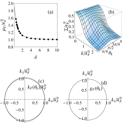
Figure 1: (a) The chemical potential, $\mu_{F}$, is plotted as a function of the unitless variable $\delta=\xi_{B}k_{F}^{0}$, where $\xi_{B}$ is the healing length [see Eq. (33)].  The dotted curve is computed self-consistently from Eqs. (27) and (28) and may be compared to the solid one which is obtained variationally from Eqs. (46) and (54). (b) The self-consistently computed Fock potential, $\Sigma\left(k,\theta_{\mathbf{k}}\right)$, for $\delta=0.8$. (c) A polar plot of the Fermi surface, $k_{F}\left(\theta_{\mathbf{k}}\right)$.  The dotted curve is extracted from the Fock potential plotted in (b) and may be compared to the solid curve which is determined variationally from Eqs. (46) and (51).  (d) A polar plot of $g_{F}\left(\theta_{\mathbf{k}}\right)$, which is defined in Eq. (40) and is proportional to the density of states at the Fermi surface. The plot in (d) is determined variationally from Eqs. (46) and (53).  In (c) and (d), the polar angle $\theta_{\mathbf{k}}$ is measured with respect to the positive $k_{z}$-axis. In each plot, we used $\lambda=0.87$ and $\varepsilon_{dd}=0.8$, where $\lambda=N\left(\epsilon_{F}^{0}\right)U_{BF}^{2}/U_{BB}$ is defined in Eq. (34), and $\varepsilon_{dd}=4\pi d^{2}/(3U_{BB})$ measures the dipolar interaction relative to the s-wave interaction.

To capture the anisotropic nature of the Fock potential, we organize the single-particle dispersion

$$\xi_{\mathbf{k}}=\frac{\hbar^{2}}{2m_{F}\gamma\left(k,\theta_{\mathbf{k}}\right)}\left[k^{2}-k_{F}^{2}\left(\theta_{\mathbf{k}}\right)\right],$$ (38)

in terms of two parameters, $k_{F}\left(\theta_{\mathbf{k}}\right)$ and $\gamma\left(k,\theta_{\mathbf{k}}\right)$, which, in principle, can always be extracted from the numerically computed Fock potential.   Physically, the former defines the Fermi surface $k=k_{F}\left(\theta_{\mathbf{k}}\right)$, while the latter allows us to define $m_{F}\gamma_{F}\left(\theta_{\mathbf{k}}\right)$ as the renormalized mass along the $\theta_{\mathbf{k}}$ direction at the Fermi surface, where $\gamma_{F}\left(\theta_{\mathbf{k}}\right)=\lim_{k\rightarrow k_{F}\left(\theta_{\mathbf{k}}\right)}\gamma\left(k,\theta_{\mathbf{k}}\right)$.  These same physical interpretations also follow from the roles these quantities play in modifying the density of states.  By definition, the number of states per unit volume, $dN$, along $\theta_{\mathbf{k}}$ within the solid differential angle $d\Omega_{\mathbf{k}}=\sin\theta_{\mathbf{k}}d\theta_{\mathbf{k}}d\phi_{\mathbf{k}}$, is given by

$$dN=\frac{1}{(2\pi)^{3}}\frac{k^{2}}{\left|\nabla_{\mathbf{k}}\xi_{\mathbf{k}}\right|}d\Omega_{\mathbf{k}}\equiv N\left(\Omega_{\mathbf{k}}\right)\frac{d\Omega_{\mathbf{k}}}{4\pi},$$ (39)

where $N\left(\Omega_{\mathbf{k}}\right)$ is defined as the density of states.  This means that in the limit where the Fermi surface varies slowly with $\theta_{\mathbf{k}}$ in the sense that $\left|k_{F}^{-1}\left(\theta_{\mathbf{k}}\right)dk_{F}\left(\theta_{\mathbf{k}}\right)/d\theta_{\mathbf{k}}\right|\ll 1$, the density of states at the Fermi surface,

$$N\left(\Omega_{\mathbf{k}}\right)=N\left(\epsilon_{F}^{0}\right)\left[g_{F}\left(\theta_{\mathbf{k}}\right)\equiv\gamma_{F}\left(\theta_{\mathbf{k}}\right)k_{F}\left(\theta_{\mathbf{k}}\right)/k_{F}^{0}\right],$$ (40)

simply corresponds to Eq. (35) for the isotropic case in which $k_{F}^{0}$ and $m_{F}$ are replaced, respectively, with $k_{F}\left(\theta_{\mathbf{k}}\right)$ and $m_{F}\gamma_{F}\left(\theta_{\mathbf{k}}\right)$.  This result is in complete agreement with our expectation in light of the discussion above.  Thus, we see that the Fock potential introduces anisotropy in the density of states so that the density of states at the Fermi surface is modulated along the angular dimension by a factor of $g_{F}\left(\theta_{\mathbf{k}}\right)$.

In the low temperature limit $k_{B}T/\epsilon_{F}^{0}\ll 1$, $k^{2}K\left(\mathbf{k}\right)$ is negligible except around the Fermi surface $k=k_{F}\left(\theta_{\mathbf{k}}\right)$, where it is sharply peaked compared to other momentum distributions inside the integration kernel in Eq. (31).  This allows us to apply an analogous procedure, well-known in the study of isotropic BCS pairing landau80 , to single out the states near the Fermi surface as the dominant contribution to the gap equation.  Indeed, we find, to a good approximation (correct up to a pre-exponential factor), that the gap at the Fermi surface $\Delta\left(\theta_{\mathbf{k}}\right)\equiv\Delta\left(k,\theta_{\mathbf{k}}\right)|_{k=k_{F}\left(\theta_{\mathbf{k}}\right)}$ obeys the equation

$$\Delta\left(\theta_{\mathbf{k}}\right) \mathbf{=}\mathbf{-}\frac{\lambda}{4\pi}\ln\frac{\pi k_{B}T}{8\epsilon_{F}^{0}e^{\gamma-2}}\times$$

$$\int g_{F}\left(\theta_{\mathbf{k}^{\prime}}\right)\bar{U}_{A}\left(\theta_{\mathbf{k}},\theta_{\mathbf{k}^{\prime}}\right)\Delta\left(\theta_{\mathbf{k}^{\prime}}\right)\sin\theta_{\mathbf{k}^{\prime}}d\theta_{\mathbf{k}^{\prime}},$$ (41)

where

$$\bar{U}_{A}\left(\theta_{\mathbf{k}},\theta_{\mathbf{k}^{\prime}}\right)\equiv\frac{U_{A}\left(k,\theta_{\mathbf{k}},k^{\prime},\theta_{\mathbf{k}^{\prime}}\right)|_{k=k_{F}\left(\theta_{\mathbf{k}}\right),k^{\prime}=k_{F}\left(\theta_{\mathbf{k}^{\prime}}\right)}}{U\left(0\right)},$$ (42)

is the matrix element of the scaled interaction between two momenta on the Fermi surface.  The critical temperature then becomes

$$T=\frac{8\epsilon_{F}^{0}e^{\gamma-2}}{\pi k_{B}}\exp\left[-\frac{1}{\omega\lambda}\right],$$ (43)

where $\omega$ is the largest positive eigenvalue of the eigenvalue equation

$$4\pi\int g_{F}\left(\theta_{\mathbf{k}^{\prime}}\right)\bar{U}_{A}\left(\theta_{\mathbf{k}},\theta_{\mathbf{k}^{\prime}}\right)\psi\left(\theta_{\mathbf{k}^{\prime}}\right)\sin\theta_{\mathbf{k}^{\prime}}d\theta_{\mathbf{k}^{\prime}}=\omega\psi\left(\theta_{\mathbf{k}}\right).$$ (44)

As can be seen, when we set $g_{F}\left(\theta_{\mathbf{k}^{\prime}}\right)=1$, we recover from Eqs. (41) and (44) the corresponding equations in the absence of Fermi surface deformation.

Inspired by the work in miyakawa08 ; fregoso09 and the fact that our numerically determined Fermi surface fits well with an ellipsoid, we assume that the Femi particle number $n_{\mathbf{k}}\equiv\left\langle\hat{a}_{\mathbf{k}}^{{\dagger}}\hat{a}_{\mathbf{k}}\right\rangle$ distributes according to the variational ansatz

$$n_{\mathbf{k}}=\Theta\left[\left(k_{F}^{0}\right)^{2}-\alpha^{-1}\left(k_{x}^{2}+k_{y}^{2}\right)-\alpha^{2}k_{z}^{2}\right],$$ (45)

where $\Theta\left[x\right]$ is the Heaviside step function, and $\alpha$ is the so-called deformation parameter; the Fermi surface is prolate when $\alpha<1$ and oblate when $\alpha>1$.  An explicit evaluation of both kinetic energy and Fock potential indicates that $\alpha$ may be determined variationally by minimizing the (kinetic + Fock exchange) energy density:

$$\mathcal{E}\left(\alpha\right)=\frac{1}{2}\frac{\hbar^{2}}{m_{F}}\frac{\left(k_{F}^{0}\right)^{5}}{10\pi^{2}}Y\left(\alpha\right),$$ (46)

where

$$Y\left(\alpha\right) =\frac{2}{3}\alpha+\frac{1}{3\alpha^{2}}$$

$$+\frac{5}{12}\lambda\text{ }\int_{0}^{\pi}I\left(\theta_{\mathbf{k}},\alpha,\varepsilon_{dd},\delta\right)\sin\theta_{\mathbf{k}}d\theta_{\mathbf{k}}.$$ (47)

In Eq. (47),

$$I\left(\theta_{\mathbf{k}},\alpha,\varepsilon_{dd},\delta\right)$$

$$=\frac{1}{4d}\left(6-\frac{c}{d}\right)-\frac{2}{d}\sqrt{\frac{c}{d}}\tan^{-1}\left(2\sqrt{\frac{d}{c}}\right)$$

$$+\frac{1}{16d}\frac{c}{d}\left(\frac{c}{d}+12\right)\ln\left(1+4\frac{d}{c}\right)$$ (48)

plays the same role as the deformation function in dipolar Fermi gases miyakawa08 , but with a more complicated form that depends not only on the deformation parameter $\alpha$ but also on $\varepsilon_{dd}$ and $\delta$,  where

$$c =1-\varepsilon_{dd}+3\varepsilon_{dd}\frac{\cos^{2}\theta_{\mathbf{k}}}{\alpha^{3}\sin^{2}\theta_{\mathbf{k}}+\cos^{2}\theta_{\mathbf{k}}}\text{ ,}$$ (49)

$$d =\frac{\delta^{2}}{\alpha^{2}}\left(\alpha^{3}\sin^{2}\theta_{\mathbf{k}}+\cos^{2}\theta_{\mathbf{k}}\right).$$ (50)

For an ellipsoid whose Fermi surface is defined by Eq. (45),

$$k_{F}\left(\theta_{\mathbf{k}}\right) \equiv k_{F}^{0}\left(\alpha^{-1}\sin^{2}\theta_{\mathbf{k}}+\alpha^{2}\cos^{2}\theta_{\mathbf{k}}\right)^{-1/2},$$ (51)

$$\gamma_{F}\left(\theta_{\mathbf{k}}\right) =\left(\alpha^{-1}\sin^{2}\theta_{\mathbf{k}}+\alpha^{2}\cos^{2}\theta_{\mathbf{k}}\right)^{-1},$$ (52)

and consequently according to Eq. (40)

$$g_{F}\left(\theta_{\mathbf{k}}\right)=\left(\alpha^{-1}\sin^{2}\theta_{\mathbf{k}}+\alpha^{2}\cos^{2}\theta_{\mathbf{k}}\right)^{-3/2}.$$ (53)

The corresponding chemical potential, calculated using $\mu_{F}=\partial\mathcal{E}/\partial n_{F}$, is found to be

$$\frac{\mu_{F}}{\epsilon_{F}^{0}} =\frac{6}{5}Y\left(\alpha\right)-\frac{1}{5}\left(\frac{2}{3}\alpha+\frac{1}{3\alpha^{2}}\right)$$

$$+\frac{1}{12}\lambda\int_{0}^{\pi}K\left(\theta_{\mathbf{k}},\alpha,\varepsilon_{dd},\delta\right)\sin\theta_{\mathbf{k}}d\theta_{\mathbf{k}},$$ (54)

where

$$K\left(\theta_{\mathbf{k}},\alpha,\varepsilon_{dd},\delta\right)$$

$$=3\left(\frac{c}{2d^{2}}-\frac{1}{d}\right)+6\frac{\sqrt{c}}{d^{3/2}}\tan^{-1}\left(2\frac{d^{1/2}}{\sqrt{c}}\right)$$

$$-\frac{c}{8}\left(\frac{3c}{d^{3}}+\frac{24}{d^{2}}\right)\ln\left(1+\frac{4}{c}d\right).$$ (55)

Figure 1(a) shows that Eq. (54) produces a chemical potential (solid curve) that is in good agreement with the one obtained self-consistently from Eqs. (27) and (28) (dots).  Figure 1(c) shows that compared to the self-consistent method (dotted curve), the variational method (black curve) underestimates the prolateness of the Fermi surface, but nonetheless captures the essential anisotropic feature of the Fermi surface and does not, in our judgement, prevent us from using it as a computationally economic tool for estimating the critical temperature.

Our algorithm for computing the critical temperature is then as follows: we first calculate $\alpha$ by minimizing Eq. (46) with respect to $\alpha$; next we use it to fix $g_{F}\left(\theta_{\mathbf{k}}\right)$ according to Eq. (53); we then substitute $g_{F}\left(\theta_{\mathbf{k}}\right)$ into Eq. (44) to determine the eigenvalue $\omega$; finally we use Eq. (43) to estimate the critical temperature.  Figure 2 (a) compares the eigenvalue in the absence of dipolar interaction (dashed curve) with those in the presence of dipolar interaction (solid curves), indicating that in contrast to the former, which asymptotes to zero, in the limit of small $\delta$, the latter approach finite values, which increase dramatically with the increase in $\varepsilon_{dd}$.  This is explicitly shown in Fig. 2 (b), which is a plot of the critical temperature for various $\varepsilon_{dd}$.  Not shown in Fig. 2(b) is the critical temperature in the absence of the dipolar interaction, which is orders of magnitude lower.

Figure 2: The superfluid critical temperature, $T$, is proportional to $\exp\left(-1/\omega\lambda\right)$ [Eq. (43)], where $\omega$ is the largest positive eigenvalue of Eq. (44) and $\lambda=N\left(\epsilon_{F}^{0}\right)U_{BF}^{2}/U_{BB}$ is defined in Eq. (34).  (a) The eigenvalue, $\omega$, is plotted as a function of the unitless variable $\delta=\xi_{B}k_{F}^{0}$, where $\xi_{B}$ is the healing length [see Eq. (33)].  The dashed curve corresponds to the absence of the dipolar interaction ($\varepsilon_{dd}=0$).  The solid curves, from bottom to top, correspond to $\varepsilon_{dd}$ = $0.1,$ $0.2$, 0.5 and 0.8, where $\varepsilon_{dd}=4\pi d^{2}/(3U_{BB})$ measures the dipolar interaction relative to the s-wave interaction. (b) The critical temperature, $T$, in the units of $T_{F}^{0}\equiv\epsilon_{F}^{0}/k_{B}$ is plotted as a function of $\delta$.  The curves, from bottom to top, correspond to $\varepsilon_{dd}$=0.6, 0.7 and 0.8.  All curves are produced with $\lambda=0.87$.

IV Optimal critical temperature prior to phase separation

The issue of whether different phases can coexist in the same spatial volume (miscibility) or repel each other into separate spatial regions (phase separation) will inevitably arise when one is considering systems made up of quantum gases with different species.  The knowledge of phase separation is essential before one can apply the theory developed in the previous sections to estimate the critical temperature achievable before the system starts to phase separate. An understanding of the phase separation, even in view of the tremendous simplification due to the use of the variational method, would most likely remain a computationally expensive endeavor if one were to take into full consideration the Fock potential.  Consequently, when studying phase separation we choose to ignore the momentum dependence of the induced interaction by assuming $U\left(\mathbf{k}\right)=U\left(0\right)$.  The modification due to this assumption is not expected to undermine our goal (in this section) of gaining a qualitative understanding about the order of magnitude of the achievable critical temperature.  This assumption allows the Fock potential to cancel the Hartree potential identically, leading to a much simplified $\Omega$, which, when expressed in terms of $A=$ $\hbar^{2}\left(6\pi^{2}\right)^{2/3}/2m_{F}$, takes the form

$$\Omega =\frac{1}{2}U_{BB}n_{B}^{2}-u_{B}n_{B}+U_{BF}n_{B}n_{F}$$

$$+\frac{3}{5}An_{F}^{5/3}-u_{F}n_{F},$$ (56)

where we have used Eqs. (11), (22), (24) and (27), and ignored $\Omega_{1}$, the energy contribution from Cooper pairs, as we have done in other sections.

Note that Eq. (56) has the same mathematical form as the one for a homogeneous Fermi-Bose mixture model, which has been extensively analyzed in efremov02 ; viverit00 .  Here, we recapture the main physics by performing the same analysis but in the chemical potential space fodor10 . Consider first the mixed phase where both $n_{B}$ and $n_{F}$ have finite values. The corresponding chemical potentials are given by

$$u_{B} =\frac{\partial\Omega}{\partial n_{B}}=U_{BB}n_{B}+U_{BF}n_{F},$$ (57)

$$u_{F} =\frac{\partial\Omega}{\partial n_{F}}=U_{BF}n_{B}+An_{F}^{2/3}.$$ (58)

Eliminating the boson density, we arrive at a cubic equation for $n_{F}^{1/3}$,

$$\frac{U_{BF}^{2}}{U_{BB}}\left(n_{F}^{1/3}\right)^{3}-A\left(n_{F}^{1/3}\right)^{2}+u_{F}-\frac{U_{BF}}{U_{BB}}u_{B}=0,$$ (59)

which allows us to determine $n_{F}^{1/3}$ given a set of $u_{F}$ and $u_{B}$. Not all positive solutions to Eq. (59) are stable and therefore physically realizable; the values of $n_{F}^{1/3}$ are constrained by the stability condition which requires the following Hessian matrix to be positive semidefinite:

$$\left(\begin{array}[c]{cc}\frac{\partial^{2}\Omega}{\partial n_{B}^{2}}&\frac{\partial^{2}\Omega}{\partial n_{B}\partial n_{F}}\\ \frac{\partial^{2}\Omega}{\partial n_{F}\partial n_{B}}&\frac{\partial^{2}\Omega}{\partial n_{F}^{2}}\end{array}\right)=\left(\begin{array}[c]{cc}U_{BB}&U_{BF}\\ U_{BF}&A\frac{2}{3}\frac{1}{n_{F}^{1/3}}\end{array}\right),$$ (60)

or equivalently

$$n_{F}^{1/3}<A\frac{2U_{BB}}{3U_{BF}^{2}}.$$ (61)

There exists only one positive root to the cubic equation (59) that satisfies the stability condition and this happens in the chemical potential space when

$$\frac{U_{BF}}{U_{BB}}u_{B}<u_{F}<\frac{U_{BF}}{U_{BB}}u_{B}+\frac{4}{27}\frac{A^{3}U_{BB}^{2}}{U_{BF}^{4}}.$$ (62)

This means that there is a unique mixed state, which precludes the possibility of phase separation involving more than one mixed phase.

Next,  in the region that supports a pure Bose phase, the effective chemical potential for fermions shall be less than zero, $u_{F}-U_{BF}n_{B}<0$, which, when combined with $u_{B}=U_{BB}n_{B}$ for a pure Bose state, shows immediately that the pure Bose phase exists in the chemical potential space with

$$u_{F}<U_{BF}u_{B}/U_{BB}.$$ (63)

Thus, we see that there is no overlap between the pure Bose and the mixed phase; the two phases are divided by the line $u_{F}=U_{BF}u_{B}/U_{BB}$, which is second order in nature.  As a result, phase separation between the mixed state and a pure Bose state is impossible.

The only remaining possibility is phase separation between a mixed state with densities $\left(n_{F1},n_{B1}\right)$ and a pure Fermi phase with densities $\left(n_{F2},n_{B2}=0\right)$.  (A complete separation between fermions and bosons requires much higher densities than considered in the present work.)  The mixed phase must share the same chemical and thermodynamical potentials with the pure phase, meaning

$$U_{BF}n_{B1}+An_{F1}^{2/3} =An_{F2}^{2/3},$$ (64)

$$U_{BB}n_{B1}^{2}/2+U_{BF}n_{B1}n_{F1}+\frac{2}{5}An_{F1}^{5/3} =\frac{2}{5}An_{F2}^{5/3},$$ (65)

from which we find

$$n_{B1}=\frac{A}{U_{BF}}n_{F1}^{2/3}\left(y^{2}-1\right),$$ (66)

where $y=\left(n_{F2}/n_{F1}\right)^{1/3}$ is the solution to the equation

$$-\frac{15}{\lambda}\left(y+1\right)^{2}+8y^{3}+16y^{2}+24y+12=0\text{,}$$ (67)

where $\lambda$ is given by Eq. (34) except that $\epsilon_{F}^{0}$ is replaced with the Fermi energy $\epsilon_{F1}^{0}$ of the mixed phase.  The stability condition in Eq. (61) then means that the stable mixture takes place when $\lambda$ $<1$.

Let us now turn to the question of how to identify the parameter space which optimizes the critical temperature before the system phase separates.  A possible solution can be found in Ref. efremov02 .  Here, we offer an answer from a different perspective. To be concrete, we consider a system in which $m_{F}=6$ amu, $m_{B}=127$ amu, $a_{BB}=250a_{0}$ (with amu being the atomic mass unit and $a_{0}$ the Bohr radius). Our task here is to find, for a given $\lambda$ and $\varepsilon_{dd}$, a set of $\left(n_{F,}n_{B},a_{BF}\right)$ which optimize the critical temperature before the system phase separates.  We begin with Eq. (43), the equation for the critical temperature.  We replace $\epsilon_{F}^{0}$ in Eq. (43) in favor of $\delta$ defined in Eq. (33) and reorganize Eq. (43) in terms of $\delta$ as

$$T=e^{\gamma-2}\frac{8^{2}\hbar^{2}n_{B}a_{BB}}{k_{B}m_{F}}\left\{\tilde{T}\left(\delta\right)=\delta^{2}\exp\left[-\frac{1}{\omega\left(\delta\right)\lambda}\right]\right\},$$ (68)

where the argument in $\omega\left(\delta\right)$ is to stress that when $\lambda$ and $\varepsilon_{dd}$  are fixed, the eigenvalue $\omega$ is a function of $\delta$ only.  On the one hand, in the limit of large $\delta$, $\omega\left(\delta\right)$ is a small (positive) number [See Fig. 2(a)], and thus $\tilde{T}\left(\delta\right)$ will be low due to the exponential factor in Eq. (68). On the other hand, in the limit of small $\delta$, $\tilde{T}\left(\delta\right)$ is also low due to the factor $\delta^{2}$ in Eq. (68).   Thus,  there will exist some $\delta=$ $\delta_{peak}$ at which $\tilde{T}\left(\delta\right)$ reaches a maximum value, $\tilde{T}\left(\delta_{peak}\right)$.  Once $\delta$ is fixed to $\delta_{peak}$, the temperature $T$ according to Eq. (68) increases with the boson density $n_{B}$,  and is highest when the largest $n_{B}$ is used.  Provided that $n_{B}$ does not exceed values where three-body recombination begins to dominate the loss mechanism, the highest possible $n_{B}$ before phase separation equals $n_{B1}$ in Eq. (66) when $n_{F1}=n_{F}$.  Finally, by combining Eq. (66) with Eqs. (33), (34) and (36), and solving them simultaneously, we find that the required $\left(n_{F,}n_{B},a_{BF}\right)$ are given by

$$n_{F} =\frac{\pi}{6\left(8^{3}\right)}\frac{\lambda^{3}\left(m_{F}/m_{B}\right)^{3}}{a_{BB}^{3}\delta_{peak}^{12}\left(y^{2}-1\right)^{6}},$$ (69)

$$n_{B} =\frac{\pi}{2\left(8^{3}\right)}\frac{\lambda^{2}\left(m_{F}/m_{B}\right)^{2}}{a_{BB}^{3}\delta_{peak}^{10}\left(y^{2}-1\right)^{4}},$$ (70)

$$a_{BF} =2a_{BB}\delta_{peak}^{2}\frac{m_{BF}}{m_{F}}\left(y^{2}-1\right),$$ (71)

where $y$ is the solution to Eq. (67) for the given $\lambda$. The results of this optimization procedure are summarized in Fig. 3.  A comparison between Figs. 3(a) and (b) indicates that mixing fermions with a dipolar condensate can result in a dramatic increase in the achievable temperature $T$ compared to mixing fermions with a nondipolar condensate; the order of magnitude in T can be 100 nK for the former and only a fraction of 1 nK for the latter.  Figures 3(c) and (d) display, respectively, the $a_{BF}$ and $\left(n_{B},n_{F}\right)$ required to realize the temperature in Fig. 3(b) when $\varepsilon_{dd}=0.8$ (solid curve).  For example, when $\lambda=0.874$, a system with $a_{BF}=275a_{0}$, $n_{B}=2.76\times 10^{14}$ cm^-3 and $n_{F}=6.88\times 10^{12}$ cm^-3 has a critical temperature of $80$ nK.

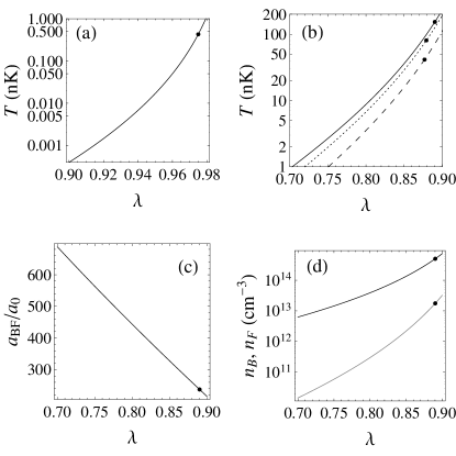
Figure 3: (a) In the absence of the dipolar interaction ($\varepsilon_{dd}=0$), the superfluid critical temperature, $T$, is plotted as a function of the unitless variable $\lambda$, where $\lambda=N\left(\epsilon_{F}^{0}\right)U_{BF}^{2}/U_{BB}$ is defined in Eq. (34). (b) For a nonzero dipolar interaction the critical temperature, $T$, is plotted for $\varepsilon_{dd}=0.6$ (long dash), 0.7 (short dash), and 0.8 (solid), where $\varepsilon_{dd}=4\pi d^{2}/(3U_{BB})$ measures the dipolar interaction relative to the s-wave interaction.  (c) $a_{BF}$ and (d) densities $n_{B}$ [black curve in (d)] and $n_{F}$ [gray curve in (d)] that are required to produce the (optimal) critical temperature for $\varepsilon_{dd}=0.8$, represented by the solid curve in (b).  The black dots mark the points at which $n_{B}$ has reached $5\times 10^{14}$ cm^-3.  All curves are produced with $m_{F}=6$ amu, $m_{B}=127$ amu, and $a_{BB}=250a_{0}$.

V Conclusion

The ability to easily mix cold atoms of different species opens up another exciting avenue for engineering quantum systems with novel properties. Mixing a dipolar condensate can induce, between two fermions in a Fermi quantum gas, an effective attractive interaction which, owning to its anisotropic nature, can dramatically enhance the scattering of fermions in the odd-parity channels.  We have explored such an interaction for the purpose of achieving, in a mixture between a spin-polarized Fermi gas and a dipolar condensate, a superfluid with a gap parameter characterized with a coherent superposition of all odd partial waves.  We have focused our effort on determining the critical temperature, a task far more challenging for our model than for pure fermionic systems since, first, adding dipolar bosons to fermions dramatically increases the system parameter space and, second, the system may phase separate.  We have formulated, in the spirit of the Hartree-Fock-Bogoliubov mean-field approach, a theory which allows us to treat calculating the critical temperature and phase separation in a unified manner.   We have applied this theory to estimate the critical temperature when the anisotropic Fock potential is taken into consideration and to identify the parameter space which optimizes the critical temperature before the system begins to phase separate.

VI Acknowledgement 

H. Y. L. acknowledges the support from the US National Science Foundation and the US Army Research Office.

References

- (1) L. D. Landau and E. M. Lifshitz, Quantum Mechanics: Non-Relativitic Theory (Pergamon Press, Oxford, 1977, 3rd ed.)
- (2) J. L. Bohn, Phys. Rev. A 61, 053409 (2000).
- (3) F. R. Klinkhamer and G. E. Volovik, JETP Lett. 80, 389 (2004).
- (4) Y. Ohashi, Phys. Rev. Lett. 94, 050403 (2005).
- (5) T. L. Ho and R. B. Diener, Phys. Rev. Lett. 94, 09402 (2005).
- (6) C. A. Regal, C. Ticknor, J. L. Bohn, and D. S. Jin, Phys. Rev. Lett. 90, 053201 (2003).
- (7) J. Zhang, E. G. M. van Kempen, T. Bourdel, L. Khaykovich, J. Cubizolles, F. Chevy, M. Teichmann, L. Tarruell, S. J. J. M. F. Kokkelmans, and C. Salomon, Phys. Rev. A 70, 030702 (R) (2004).
- (8) C. Ticknor, C. A. Regal, D. S. Jin, and J. L. Bohn, Phys. Rev. A 69, 042712 (2004).
- (9) K. Günter, T. Stöferle, H. Moritz, M. Köhl, and T. Esslinger, Phys. Rev. Lett. 95, 230401 (2005).
- (10) M. Marinescu and L. You, Phys. Rev. Lett. 81, 4596 (1998);L. You and M. Marinescu, Phys. Rev. A 60, 2324 (1999).
- (11) M. A. Baranov, M. S. Mar’enko, Val. S. Rychkov, and G. V. Shlyapnikov, Phys. Rev. A 66, 013606 (2002); M. A. Baranov, L. Dobrek, and M. Lewenstein, Phys. Rev. Lett. 92, 250403 (2004).
- (12) K. V. Samokhin and M. S. Mar’enko, Phys. Rev. Lett. 197003 (2006).
- (13) G. M. Bruun and E. Taylor, Phys. Rev. Lett. 101, 245301 (2008); G. M. Bruun and E. Taylor, Phys. Rev. Lett. 107, 169901 (2011).
- (14) C. Wu and J. E. Hirsch, Phys. Rev. B 81, 020508 (R) (2010).
- (15) T. Shi, J.-N. Zhang, C.-P. Sun, and S. Yi, Phys. Rev. A 82, 033623 (2010)
- (16) R. Liao and J. Brand, Phys. Rev. A, 82, 063624 (2010).
- (17) S. Ronen and J. L. Bohn, Phys. Rev. A 81, 033601 (2010).
- (18) C. Zhao, L. Jiang, X. Liu, W. M. Liu, X. Zou, and H. Pu, Phys. Rev. A 81, 063642 (2010).
- (19) S. Ospelkaus, A. Pe’er, K.-K. Ni, J. J. Zirbel, B. Neyenhuis, S. Kotochigova, P. S. Julienne, J. Ye, and D. S. Jin, Nature Phys. 4 , 622 (2008).
- (20) K. K. Ni, S. Ospelkaus, M. H. G. de Miranda, A. Pe’er, B. Neyenhuis, J. J. Zirbel, S. Kotochigova,P. S. Julienne, D. S. Jin, and J. Ye, Science 322, 231 (2008).
- (21) S. Ospelkaus, K. K. Ni, M. H. G. de Miranda, B. Neyenhuis, D. Wang, S. Kotochigova, P. S. Julienne, D. S. Jin, and J. Ye, Faraday Discuss. 142, 351 (2009).
- (22) J. Stuhler, A. Griesmaier, T. Koch, M. Fattori, T. Pfau, S. Giovanazzi, P. Pedri, and L. Santos, Phys. Rev. Lett. 95, 150406 (2006).
- (23) M. Vengalattore, S. R. Leslie, J. Guzman, and D. M. Stamper-Kurn, Phys. Rev. Lett. 100, 170403 (2008).
- (24) M. Lu, N. Q. Burdick, S. H. Youn, and B. L. Lev, Phys. Rev. Lett. 107, 190401 (2011).
- (25) Y.-il Shin, A. Schirotzek, C. H. Schunck, and W. Ketterle, Phys. Rev. Lett. 101, 070404 (2008).
- (26) J. W. Park, C.-H Wu, I. Santiago, T. G. Tiecke, P. Ahmadi, M. W. Zwierlein, e-print arXiv:1110.4552 (2011).
- (27) C.-H. Wu, I. Santiago, J. W. Park, P. Ahmadi, and M. W. Zwierlein, Phys. Rev. A. 84, 011601(R) (2011).
- (28) M. J. Bijlsma, B. A. Heringa, and H. T. C. Stoof, Phys. Rev. A 61, 053601 (2000).
- (29) D. V. Efremov and L. Viverit, Phys. Rev. B 65, 134519 (2002).
- (30) O. Dutta and M. Lewenstein, Phys. Rev. A 81, 063608 (2010).
- (31) C. Nayak, S. H. Simon, A. Stern, M. Freedman, S. Das Sarma, Rev. Mod. Phys. 80, 1083 (2008).
- (32) Y. Nishida, Annals Phys. 324, 897 (2009).
- (33) Y. Nishida, and S. Tan, Phys. Rev. A 82, 062713 (2010).
- (34) B. Kain and H. Y. Ling, Phys. Rev. A 83, 061603(R).
- (35) K. Góral, K. Rza̧żewski, and T. Pfau, Phys. Rev. A 61, 051601 (2000).
- (36) S. Giovanazzi, A. Görlitz, and T. Pfau, Phys. Rev. Lett. 89, 130401 (2002).
- (37) D. H. J. O’Dell, S. Giovanazzi, and C. Eberlein, Phys. Rev. Lett. 92, 250401 (2004).
- (38) C.-K. Chan, C. Wu, W.-C. Lee, and S. Das Sarma, Phys. Rev. A 81, 023602 (2010).
- (39) P. G. de Gennes, Superconductivity of Metals and Alloys (Addison-Wesley Publishing Company, New York, 1989).
- (40) L. D. Landau and E. M. Lifshitz, Statistical Physics, Part 2 (Butterworth-Heinemann, Oxford, 1980).
- (41) T. Miyakawa, T. Sogo, and H. Pu, Phys. Rev. A 77, 061603(R) (2008); T Sogo, L He, T Miyakawa, S Yi, H Lu and H Pu, N. J. Phys. 11, 055017 (2009).
- (42) B. M. Fregoso, K. Sun, E. Fradkin and B. L Lev, New J. Phys. 11, 103003 (2009).
- (43) L. Viverit,C. J. Pethick, and H. Smith, Phys. Rev. A bf 61, 053605 (2000).
- (44) M. Fodor and H. Y. Ling, Phys. Rev. A 82, 043610 (2010).