Bayesian Model Robustness via Disparities
Abstract
This paper develops a methodology for robust Bayesian inference through the use of disparities. Metrics such as Hellinger distance and negative exponential disparity have a long history in robust estimation in frequentist inference. We demonstrate that an equivalent robustification may be made in Bayesian inference by substituting an appropriately scaled disparity for the log likelihood to which standard Monte Carlo Markov Chain methods may be applied. A particularly appealing property of minimum-disparity methods is that while they yield robustness with a breakdown point of 1/2, the resulting parameter estimates are also efficient when the posited probabilistic model is correct. We demonstrate that a similar property holds for disparity-based Bayesian inference. We further show that in the Bayesian setting, it is also possible to extend these methods to robustify regression models, random effects distributions and other hierarchical models. The methods are demonstrated on real world data.
1 Introduction
In this paper we develop a new methodology for providing robust inference in a Bayesian context. When the data at hand are suspected of being contaminated with large outliers it is standard practice to account for these either (1) by postulating a heavy-tailed distribution, (2) by viewing the data as a mixture, with the contamination explicitly occurring as a mixture component or (3) by employing priors that penalize large values of a parameter (see Berger, 1994; Albert, 2009; Andrade and O’Hagan, 2006). In the context of frequentist inference, these issues are investigated using methods such as M-estimation, R-estimation etc. and are part of standard robustness literature (see Hampel et al., 1986; Maronna et al., 2006; Jur, ). As is the case for Huberized loss functions in frequentist inference, even though these approaches provide robustness they lead to a loss of precision when contamination is not present in (1) and (2) above or to a distortion of prior knowledge in (3). Explicit modeling of outliers as in (2) also requires knoweldge of outlier configurations – how many mixture components to use and what distributions to use them in, for example – and may not be robust if these are incorrect. This paper develops an alternative systematic Bayesian approach, based on disparity theory, that is shown to provide robust inference without loss of efficiency for large samples.
In parametric frequentist inference using independent and identically distributed (i.i.d.) data, several authors (Beran, 1977; Tamura and Boos, 1986; Simpson, 1987, 1989; Cheng and Vidyashankar, 2006) have demonstrated that the dual goal of efficiency and robustness is achievable by using the minimum Hellinger distance estimator (MHDE). In the i.i.d. context, MHDE estimators are defined by minimizing the Hellinger distance between a postulated parametric density and a non-parametric estimate over the -dimensional parameter space ; that is,
| (1) |
Typically, for continuous data, is taken to be a kernel density estimate; if the probability model is supported on discrete values, the empirical distribution is used. More generally, Lindsay (1994) introduced the concept of a minimum disparity procedure; developing a class of divergence measures that have similar properties to minimum Hellinger distance estimates. These have been further developed in Basu et al. (1997) and Park and Basu (2004). Hooker and Vidyashankar (2010a) have extended these methods to a regression framework.
A remarkable property of disparity-based estimates is that while they confer robustness, they are also first-order efficient. That is, they obtain the information bound when the postulated density is correct. In this paper we develop robust Bayesian inference using disparities. We show that appropriately scaled disparities approximate times the negative log-likelihood near the true parameter values. We use this as a motivation to replace the log likelihood in Bayes rule with a disparity to create what we refer to as the “D-posterior”. We demonstrate that this technique is readily amenable to Markov Chain Monte Carlo (MCMC) estimation methods. Finally, we establish that the expectation of the D-posterior is asymptotically efficient and the resulting credible intervals provide asymptotically accurate coverage when the proposed parametric model is correct.
Disparity-based robustification in Bayesian inference can be naturally extended to a regression framework through the use of conditional density estimation as discussed in Hooker and Vidyashankar (2010a). We pursue this extension to hierarchical models and replace various terms in the hierarchy with disparities. This creates a novel “plug-in procedure” – allowing the robustification of inference with respect to particular distributional assumptions in complex models. We develop this principle and demonstrate its utility on a number of examples. The use of a disparity within a Bayesian context imposes an additional computational burden through the estimation of a kernel density estimate and the need to run MCMC methods. Our analysis and simulations demonstrate that while the use of MCMC significantly increases computational costs, the additional cost of the use of disparities is on the order of a factor between 2 and 10, remaining implementable for many applications. These methods require marginalization of an exponentiated disparity with respect to the random effects distribution; a task that can be achieved through MCMC methods, but would otherwise be numerically challenging.
The use of divergence measures for outlier analysis in a Bayesian context has been considered in Dey and Birmiwal (1994) and Peng and Dey (1995). Most of this work is concerned with the use of divergence measures to study Bayesian robustness when the priors are contaminated and to diagnose the effect of outliers. These divergence measures are computed using MCMC techniques. More recently, Zhan and Hettmansperger (2007) and Szpiro et al. (2010) have developed analogues of R-estimates and Bayesian Sandwich estimators. These methods can be viewed to be extensions of robust frequentist methods to Bayesian context. By contrast, our paper is based on explicitly replacing the likelihood with a disparity in order to provide a systematic approach to obtain inherently robust and efficient inference.
Within the context of Bayesian analysis, robustness has been studied with respect to the specification of both prior and data distributions. Robustness to outliers as studied in the frequentist literature is referred to as “outlier-rejection” in Bayesian analysis and is studied for example in Dawid (1973), O’Hagan (1979), O’Hagan (1990), Choy and Smith (1997) and Desgagnè and Angers (2007). Here, outlier rejection indicates that as some group of data is moved to infinity, the posterior reverts to the posterior without those observations. This corresponds to a breakdown point of 1; a rather extreme value for frequentist robustness. We also obtain this breakdown point, but additionally develop a notion of an asymptotic breakdown point in which we examine the worst-case displacement as sample-size increases. We are able to show that this notion effectively describes robustness and distinguishes Bayesian methods along with regularized versions of robust estimators from estimators that are trivially made robust by, for example, threshholding their estimates.
The remainder of the paper is structured as follows: we provide a formal definition of the disparities in Section 2. Disparity-based Bayesian inference are developed in Section 3. Robustness and efficiency of these estimates are demonstrated theoretically and through a simulation for i.i.d. data in Section 5. The methodology is extended to regression models in Section 6. The plug-in procedure is presented in Section 7 through an application to a one-way random-effects model. Section 8 is devoted to two real-world data sets where we apply these methods to generalized linear mixed models and a random-slope random-intercept models for longitudinal data. Proofs of technical results and details of simulation studies are relegated to an online appendix.
2 Disparities and Their Numerical Approximations
In this section we describe a class of disparities and numerical procedures for evaluating them. These disparities compare a proposed parametric family of densities to a non-parametric density estimate. We assume that we have i.i.d. observations for from some density . We let be the kernel density estimate:
| (2) |
where the kernel density and is a bandwidth for the kernel. If and it is known that is an -consistent estimator of (Devroye and Györfi, 1985). In practice, a number of plug-in bandwidth choices are available for (e.g. Silverman, 1982; Sheather and Jones, 1991; Engel et al., 1994). For non-i.i.d. data examined in Sections 6 and 7, plug-in bandwidths can be calculated from method of moments estimates. We have found our results to be insensitive to the choice of plug-in bandwidth selector.
We begin by reviewing the class of disparities described in Lindsay (1994). The definition of disparities involves the residual function,
| (3) |
defined on the support of and a function . is assumed to be strictly convex and thrice differentiable with , and . The disparity between and is defined to be
| (4) |
An estimate of obtained by minimizing (4) is called a minimum disparity estimator. Under differentiability assumptions, this is equivalent to solving the equation
where and indicates the derivative with respect to .
This framework contains Kullback-Leibler divergence as approximation to the likelihood:
for the choice up to a constant. The squared Hellinger disparity (HD) corresponds to the choice . While robust statistics is typically concerned with the impact of outliers, the alternate problem of inliers – defined as nominally-dense regions that lack empirical data and consequently small values of – can also cause instability. It has been illustrated in the literature that HD down weighs the effect of large values of (outliers) relative to the likelihood but magnifies the effect of inliers. An alternative, the negative exponential disparity, based on the choice down weighs the effect of both outliers and inliers.
The integrals involved in (4) are not analytically tractable and the use of Monte Carlo integration to approximate the objective function has been suggested in Cheng and Vidyashankar (2006). More specifically, if are i.i.d. random samples generated from , one can approximate by
| (5) |
The can be efficiently generated in the form for a random variable generated according to and sampled uniformly from the integers . In the specific case of Hellinger distance approximation, the above reduces to
The use of a fixed set of Monte Carlo samples from when optimizing for provides a stochastic approximation to an objective function that remains a smooth function of and hence avoids the need for complex stochastic optimization. Similarly, in the present paper, we hold the constant when applying MCMC methods to generate samples from the posterior distribution in order to improve their mixing properties. If is Gaussian with , Gauss-Hermite quadrature rules can be used to avoid Monte Carlo integration, leading to improved computational efficiency in some circumstances. In this case we have
| (6) |
where the and are the points and weights for a Gauss-Hermite quadrature scheme for parameters . The choice between (5) and (6) depends on the disparity and the problem under investigation. When has many local modes, (6) can result in choosing parameters for which some quadrature point coincides with a local modes. However, (5) can be rendered unstable by the factor for far from the maximizing value of . In general, we have found (5) preferable when using Hellinger distance, but that (6) performs better with negative exponential disparity. The relative computational cost of using versus in various circumstances is discussed in Online Appendix D.
3 The D-Posterior and MCMC Methods
We begin this section by a heuristic description of the second-order approximation of by . A Taylor expansion of about has the following first two terms:
| (7) | ||||
where the second term approximates the observed Fisher Information when the bandwidth is small. The equivalent terms for are:
| (8) | ||||
Now, if is consistent, almost surely (a.s.). Observing that , from the conditions on and observing , we obtain the equality of (7) and (8). The fact that these heuristics yield efficiency was first noticed by Beran (1977) (eq. 1.1).
In the context of Bayesian methods, inference is based on the posterior
| (9) |
where and a prior density which we assume has a first moment. Following the heuristics above, in this paper we propose the simple expedient of replacing the log likelihood, , in (9) with a disparity:
| (10) |
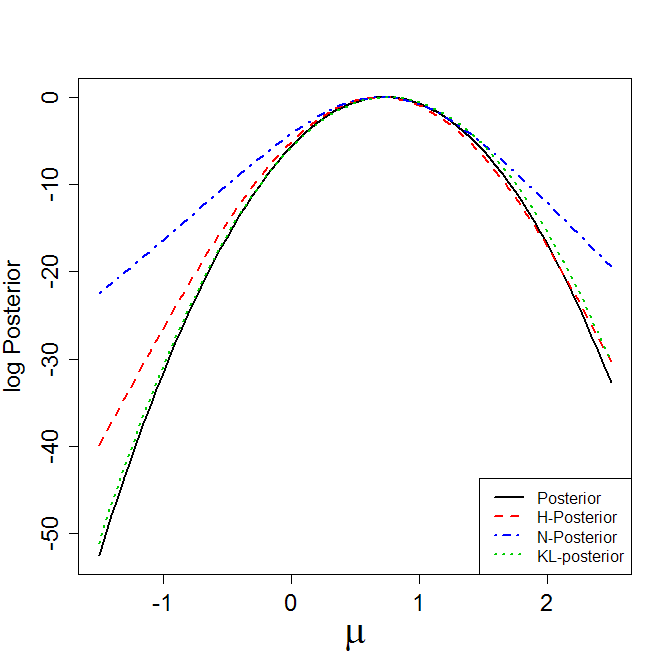
In the case of Hellinger distance, the appropriate disparity is and we refer to the resulting quantity as the H-posterior. When is based on Negative Exponential disparity, we refer to it as N-posterior, and D-posterior more generally. These choices are illustrated in Figure 1 where we show the approximation of the log likelihood by Hellinger and negative exponential disparities and the effect of adding an outlier to these in a simple normal-mean example.
Throughout the examples below, we employ a Metropolis algorithm based on a symmetric random walk to draw samples from . While the cost of evaluating is greater than the cost of evaluating the likelihood at each Metropolis step, we have found these algorithms to be computationally feasible and numerically stable. Furthermore, the burn-in period for sampling from and the posterior are approximately the same, although the acceptance rate of the former is around ten percent higher.
After substituting for the log likelihood, it will be useful to define summary statistics of the -posterior in order to demonstrate their asymptotic properties. Since the -posterior (10) is a proper probability distribution, the Expected D-a posteriori (EDAP) estimates exist and are given by
and credible intervals for can be based on the quantiles of . These quantities are calculated via Monte Carlo integration using the output from the Metropolis algorithm. We similarly define the Maximum D-a posteriori (MDAP) estimates by
In the next section we describe the asymptotic properties of EDAP and MDAP estimators. In particular, we establish the posterior consistency, posterior asymptotic normality and efficiency of these estimators and their robustness properties. Differences between and the posterior do exist and are described below:
-
1.
The disparities have strict upper bounds; in the case of Hellinger distance , the upper bound for negative exponential disparity is . This implies that the likelihood part of the D-posterior, , is bounded away from zero. Consequently, a proper prior is required in order to normalize . A random from must also have finite expectation in order for the EDAP to be defined. In particular, uniform priors on unbounded ranges, along with most reference priors, cannot be employed here. Further, the tails of are proportional to that of . As a consequence, the breakdown point for the EDAP, as traditionally defined, is 1. Although note that in Section 4 we propose an modified definition of breakdown which is appropriate for regularized and Bayesian estimators under which EDAP has a breakdown of 1/2.
These results do not affect the asymptotic behavior of since the lower bounds decrease with . Modified D-posteriors based on a transformation that removes the upper bound can be defined without affecting either the efficiency or robustness of the resulting EDAP estimates. However, appropriate transformations will depend on the the parametric family and are beyond the scope of this paper.
-
2.
In Bayesian inference for i.i.d. random variables, the log likelihood is a sum of terms. This implies that if new data are obtained, the posterior for the combined data can be obtained by using posterior after observations, as a prior :
By contrast, is generally not additive in ; hence cannot be factored as above. Extending arguments in Park and Basu (2004), we conjecture that no disparity that is additive in will yield both robust and efficient posteriors.
-
3.
While we have found that the same Metropolis algorithms can be effectively used for the D-posterior as would be used for the posterior, it is not possible to use conjugate priors with disparities. This removes the possibility of using conjugacy to provide efficient sampling methods within a Gibbs sampler, although these could be approximated by combining sampling from a conditional distribution with a rejection step.
The idea of replacing log likelihood in the posterior with an alternative criterion occurs in other settings. See Sollich (2002), for example, in developing Bayesian methods for support vector machines. However, we replace the log likelihood with an approximation that is explicitly designed to be both robust and efficient, rather than as a convenient sampling tool for a non-probabilistic model.
 |
 |
 |
4 Robustness
The appeal of disparity-based methods is that in addition to the statistical efficiency of the estimators defined above when the parametric model is correctly specified, these estimators are also robust to contamination by data taking large values. As may be expected from the results above, EDAP estimators behave similarly to their minimum-disparity counterparts at finite levels of contamination at large but finite values. However, classical measures of robustness – influence functions and breakdown points – are based at limiting values, either of infinitesimal contamination levels or contaminating values at infinity where the convergence between EDAP and minimum-disparity estimators fails. This is due to a lack of uniformity and we argue that the direct application of the robustness measures listed above do not provide an accurate description of the behavior of EDAP estimates. Instead, robustness should be measured by the properties of the pointwise limit of -level influence functions.
As noted in the introduction, robustness to outliers is treated under title of “outlier rejection” in Bayesian analysis and generally corresponds to a breakdown point of 1. As we show below, the analysis of robustness we propose also reconciles Bayesian and other regularized estimates with the traditional description of a robust estimator as having breakdown point of 1/2. A Bayesian analysis of outlier rejection for our methods can be undertaken using the analysis techniques developed here; it is omitted for the sake of brevity.
To describe robustness, we view our estimates as functionals mapping the space of densities to . In particular, we examine the EDAP estimate
| (11) |
and note that in contrast to classical approaches to analyzing robustness the interaction between the disparity and the prior requires us to make the dependence of on explicit. This dependence is shared by any estimator that incorporates priors – including all classical Bayesian methods – and affects the traditional measures of robustness as examined below. Note that here, is taken to be a deterministic sequence of maps for the space of densities to .
We analyze the behavior of under the sequence of perturbations for a sequence of densities and . Here we assume that is a contaminating sequence defined so that it becomes orthogonal to both and the parametric family for large . Note that unlike our examination of efficiency below, in these analyzes we do not require that belongs to the parametric family; thus describes the effect of adding outliers to a fixed kernel density estimate. We also assume that and become orthogonal at large values of .
| (12) | |||
| (13) | |||
| (14) |
Typically, is taken to be a uniform distribution on a small neighborhood centered at ; but these conditions are clearly more general. They extend those given in Park and Basu (2004) in not requiring to be a member of the parametric family . The -level influence function is then defined analogously to Beran (1977) by
| (15) |
where we again note that the dependence of on is induced by the prior.
(15) represents a complete description of the behavior of our estimator in the presence of contamination, up to the shape of the contaminating density. While for EDAP estimators it contains an explicit dependence on , we begin by observing its limit for large . Firstly, as with more classical Bayesian estimates, EDAP estimators approach their frequentist counterparts at a rate.
Theorem 1.
Assume that has four continuous derivatives, that is four times continuously differentiable in and that the third derivatives of are bounded. Define as in (11) and the minimum disparity estimator (MDE) as
| (16) |
then .
As an immediate corollary, the -level influence functions converge at the same rate
Corollary 1.
That is, the influence function for represents a reasonable description of the behavior of . In particular, in the case of Hellinger distance methods, Theorems 5 and 6 in Beran (1977) have direct analogues for EDAP and MDAP estimators respectively.
While Corollary 1 motivates using the properties of to describe the robustness of of , we note that the convergence in (17) need not be uniform in . The classical summaries of robustness properties investigated below are focussed on extremal values of ; the breakdown point at large and the classical influence function at small . The lack of uniformity in (17) means that these summaries when applied at finite values of need not reflect the asymptotic properties as described in . We explore this discrepancy below and argue that the asymptotic influence measure is more appropriate in the sense of representing a minimax approach to robustness. The arguments employed here are broadly applicable to robust estimators that depend on ; in particular, regularized versions of robust estimators are susceptible to the same discrepancies and our analysis provides a framework for describing robustness in this context as well.
4.1 Breakdown Point
We begin by motivating a version of the breakdown point for -dependent estimators. Classically, the breakdown point is defined to be
| (18) |
(see Huber (1981)). Beran (1977) and Park and Basu (2004) demonstrated that the MDE has a breakdown point of in the case of Hellinger distance and when and are bounded respectively. In contrast, we show in Theorem 3 and Corollary 2 below that for each fixed , . The distinction between these cases motivates an alternative measure that captures the intuition of the classical breakdown point when applied to a sequence of estimators that changes over . We define the asymptotic breakdown point of the sequence , as follows
| (19) |
That is, for each we consider the maximal displacement under -level contamination and declare a breakdown if the limit of these displacements is unbounded.
It is easy to see that MDAP estimators have asymptotic breakdown 1/2 if their MDE counterparts do and convex. Writing the MDAP estimator as
| (20) |
it is readily seen that if maximizes then for sufficiently large and thus if is uniformly bounded, so is the influence function of . Nonetheless, the convergence of to means that if there is a sequence so that as .
For EDAP estimators a uniform identifiability condition is required. We also impose boundedness on and , but note these conditions do not hold for Hellinger distance, however, a direct argument can be given and hence in Theorem 2 below and in other results we will sometimes state that “The results also hold for Hellinger Distance”.
Theorem 2.
The identifiability condition imposed above ensures that does not more closely resemble the family than . In the analysis of Park and Basu (2004), is assumed; under these conditions . If we replace by the estimate it could happen that the inequality in (21) is reversed (ie for every there is a closer to than any member of is to ). In this case, the breakdown point of could be strictly less than 1/2.
These results are in contrast to the treatment of for fixed . Here we follow Beran (1977) in evaluating for each .
Theorem 3.
The condition that be bounded holds if is bounded; this is assumed in Park and Basu (2004) and holds for the negative exponential disparity and Hellinger distance .
For MDE’s, taking yields . For EDAP estimators, the factor generally results in a reduction in strength in the disparity relative to the prior. For Hellinger distance
since the second term in canceled in normalizing the D-posterior this is equivalent to reducing by a factor .
We note here that while the above discussion examines the behavior of for small , it can readily be extended to the following corollary
Corollary 2.
Let be bounded for all and all densities and let , then the breakdown point of the EDAP is 1.
A simple direct proof is given for this in Online Appendix A. We observe that is independent of , yielding : the prior mean.
The results at fixed indicate an extreme form of robustness that results from the fact that the disparity approximation to the likelihood is weak in its tails. This produces a lack of equivariance in the resulting estimator that appears in the third term of the asymptotic expansion as shown in Equation 34 of the online appendix. The fixed result does not distinguish our estimator from alternative estimators that are clearly problematic. In particular, the threshold estimator of the mean defined by
is also efficient and has breakdown point 1. However, by considering contamination with taken to be uniform on it is readily seen that the asymptotic breakdown point is . We might also contemplate a mean estimate based on a penalized Huber loss:
where is the Huber loss function (see Huber (1981)) and . Since increases linearly for sufficiently large, the breakdown point of is also 1, but . Of course in this case, will not be efficient.
While we have suggested that the distinction between the finite and asymptotic breakdown point is a reflection more on the definition (18) than the properties of EDAP, it does leave considerable room for the design of unbounded disparities that are nonetheless robust and which would therefore also allow the use of improper priors while still obtaining proper D-a posteriori distributions.
4.2 Influence Function
An alternative measure of robustness is given by the influence function (Hampel, 1974):
| (22) |
That this function need not always provide a useful guide to the behavior of was observed in Beran (1977) and further expanded in Lindsay (1994) who demonstrated that all MDE’s that yield efficiency share the same influence function as the MLE whatever their behavior at gross levels of contamination. The analysis in Lindsay (1994) implicitly assumes an equivariant estimator so that for any . When the effect of a prior is included in the analysis a different result is obtained at finite samples, but an equivalent limiting result can be derived.
To examine the influence function for EDAP estimators, we assume that the limit may be taken inside all integrals in (22) and obtain
where indicates expectation with respect to the D-posterior with fixed density and
Here we observe that depends on the prior . This is the case for any a posteriori estimate. also depends on the disparity employed as demonstrated in
Theorem 4.
Let be bounded and assume that
| (23) |
then .
In the case of Hellinger distance the conditions of Theorem 4 require the boundedness of which may not always hold (e.g. Beran, 1977).
Despite this strong result, in an asymptotic sense the choice of disparity and prior is indestiguishable when is assumed to lie within the model class. Expanding about provides
where is lies between and and between and , since and are and respectively. We now observe that when is in the model class,
is independent of both the disparity and the prior, as is and the limiting value of coincides with the influence function of the MLE. We also note that the next leading term in the expansion above is , which co-incides with the second-order approximation in Lindsay (1994, Eqn. 7). Unlike the case of the MDE, however, here the second order term does affect the influence function at finite .
5 Efficiency and Numerical Results
While there is a large literature on robust estimation methods, disparity-based estimation methods also achieve statistical efficiency when is a member of the parametric family . In this section, we present theoretical results for i.i.d. data to demonstrate that inference based on the D-posterior is also asympotically efficient. We also conduct a simulation study to demonstrate the finite-sample performance of these estimators.
5.1 Efficiency
We recall that under suitable regularity conditions, expected a posteriori estimators are strongly consistent, asymptotically normal and are statistically efficient; (see Ghosh et al., 2006, Theorems 4.2-4.3). Our results in this section show that this property continues to hold for EDAP estimators under regularity conditions on when the model contains the true distribution. We define
as the disparity information and the parameter that minimizes (note that here depends on ). We note that if , is exactly equal to the Fisher information for .
The proofs of our asymptotic results rely on the assumptions listed below. Among these are that minimum disparity estimators are strongly consistent and efficient; this in turn relies on further assumptions, some of which make those listed below redundant. They are given here to maximize the mathematical clarity of our arguments. We assume that are i.i.d. generated from some distribution and that a parametric family, has been proposed for where has distribution . To demonstrate efficiency, we assume
-
(A1)
; i.e. is a member of the parametric family.
-
(A2)
has three continuous derivatives with , and .
-
(A3)
There exists such that for all and
-
(A4)
is positive definite and continuous in at and continuous in with respect to the metric.
-
(A5)
For any , there exists such that
-
(A6)
The minimum disparity estimator, , satisfies almost surely and .
Our first result concerns the limit distribution for the posterior density of , which demonstrates that the D-posterior converges in to a Gaussian density centered on the minimum disparity estimator with variance . This establishes that credible intervals based on either or from will be asymptotically accurate.
Theorem 5.
Our next theorem is concerned with the efficiency and asymptotic normality of EDAP estimates.
The proofs of these theorems are deferred to the online appendix B, but the following remarks concerning the assumptions (A1)-(A6) are in order:
-
1.
Assumption A1 states that is a member of the parametric family. When this does not hold, a central limit theorem can be derived for but the variance takes a sandwich-type form; see Beran (1977) in the case of Hellinger distance. For brevity, we have followed Basu et al. (1997) and Park and Basu (2004) in restricting to the parametric case.
-
2.
Assumptions A2-A5 are required for the regularity and identifiability of the parametric family in the disparity . Note that A3 holds for Hellinger distance and if is bounded from arguments in Park and Basu (2004); other disparities may require specialized demonstrations. Specific conditions for A6 to hold are given in various forms in Beran (1977); Basu et al. (1997); Park and Basu (2004) and Cheng and Vidyashankar (2006), see conditions in Online Appendix B.
-
3.
The proofs of these results employ the same strategies as those for posterior asymptotic efficiency (see Ghosh et al., 2006, for example). However, here we rely on the second-order convergence of the disparity to the likelihood at appropriate rates and the consequent asymptotic efficiency of minimum-disparity estimators, which in turn is based on a careful analysis of non-parametric density estimates.
-
4.
Since the structure of the proof only requires second-order properties and appropriate rates of convergence, we can replace for i.i.d. data with an appropriate disparity-based term for more complex models as long as A6 can be shown hold. In particular, the results in Hooker and Vidyashankar (2010b) suggest that the disparity methods for regression problems detailed in Section 6 will also yield efficient estimates.
5.2 Simulation Studies
To illustrate the small sample performance of D-posteriors, we undertook a simulation study for i.i.d. data from Gaussian distribution. 1,000 sample data sets of size 20 from a population were generated. For each sample data set, a random walk Metropolis algorithm was run for 20,000 steps using a proposal distribution and a prior, placing the true mean one prior standard deviation above the prior mean. The kernel bandwidth was selected by the bandwidth selection in Sheather and Jones (1991). H- and N-posteriors were easily calculated by combining the KernSmooth (original by Matt Wand. R port by Brian Ripley., 2009) and LearnBayes (Albert, 2008) packages in R. We also report an experiment in which the normal log likelihood is replaced in the posterior with Tukey’s biweight objective function using a cut-point of 4.685 as a comparison to alternative robust estimators. In order to compare computational cost, we have run an MCMC chain for the normal log likelihood and report these below, even though analytic posteriors are available.
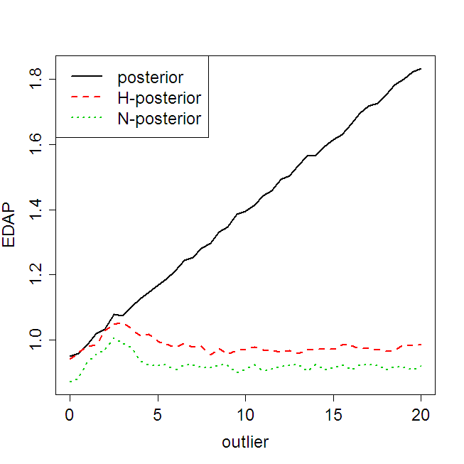
Expected a posteriori estimates for the sample mean were obtained along with 95% credible intervals from every second sample in the second half of the MCMC chain. Outlier contamination was investigated by reducing the last one, two or five elements in the data set by 3, 5 or 10. This choice was made so that both outliers and prior influence the EDAP in the same direction. The analytic posterior without the outliers is normal with mean 4.99 (equivalently, bias of -0.01) and standard deviation 0.223.
The results of this simulation are summarized in Tables 1 (uncontaminated data) and 2 (contaminated data). As can be expected, the standard Bayesian posterior suffers from sensitivity to large negative values whereas the disparity-based methods remain nearly unchanged. Tukey’s biweight also ignored large outliers, but was more sensitive than the disparity methods to larger amounts of contamination. Near-outliers at the smaller value of -3 resulted in similar biases across all methods. We observe that all robust estimates have slightly larger standard deviations than the EAP corresponding to a loss of efficiency of 2% for the H-posterior and 5% for the N-posterior and Tukey estimates. We speculate the increased variance from the N-posterior is due to its relatively Heavier tails (the maximal value of NED is compared to 4 for 2HD). A comparison of CPU time indicates that the use of disparity methods required a little more than twice the computational effort as compared to using the likelihood within an MCMC method. Further details from this simulation, including comparisons with Huber estimators are given in Online Appendix E.1.
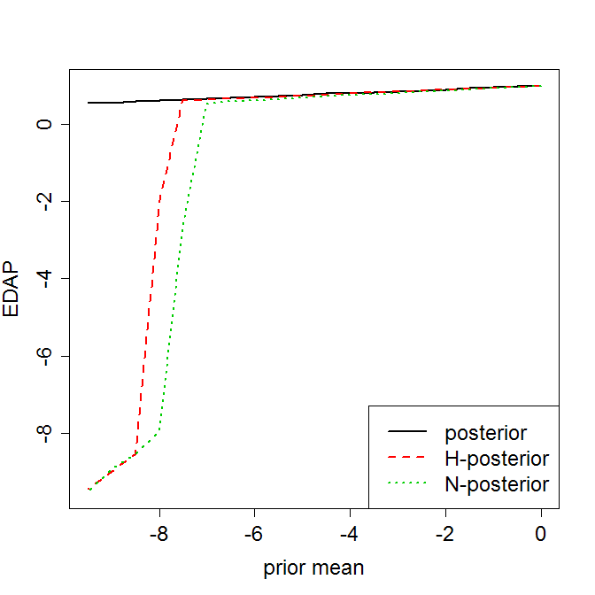
The influence of the prior is investigated in the right-hand plot of Figure 1 where we observe that the EAP and EDAP estimates are essentially identical until the prior is about 9 standard deviations from the mean of the data: at this point the prior dominates. However, we note that this picture will depend strongly on the prior chosen; a less informative prior will have a smaller range of dominance.
Because the normal distribution is symmetric, estimating its mean is relatively easy. We therefore also conducted a simulation to estimate both shape and scale parameters in an exponential-Gamma distribution (i.e. has a Gamma distribution). The details and results of this simulation are reserved to Online Appendix E.1. We observed the expected behavior: EDAP estimates remained insensitive to outliers, whereas they significantly distorted the EAP. However in this case, the H-posterior demonstrated larger variance than the N-posterior which we explain as being due to the tendency of nonparametric density estimates from exponential-Gamma data to become bimodal: producing inliers where a large value of the parametric density is compared to a relatively small value of the nonparametric estimate.
Bias SD Coverage Length CPU Time Posterior -0.015 0.222 0.956 0.873 3.393 Hellinger -0.015 0.225 0.954 0.920 7.669 Negative Exponential -0.018 0.229 0.973 1.022 7.731 Biweight -0.017 0.228 0.977 1.007 3.523
1 Outlier 2 Outliers 5 Outliers Loc Bias SD Coverage Bias SD Coverage Bias SD Coverage Posterior -3 -0.164 0.219 0.883 -0.300 0.206 0.722 -0.637 0.182 0.100 -5 -0.264 0.219 0.778 -0.490 0.206 0.375 -1.053 0.182 0.001 -10 -0.513 0.219 0.360 -0.965 0.207 0.004 -2.093 0.182 0.000 HD -3 -0.109 0.246 0.920 -0.194 0.275 0.859 -0.237 0.299 0.770 -5 -0.027 0.238 0.942 -0.040 0.257 0.928 -0.024 0.305 0.865 -10 -0.014 0.234 0.948 -0.019 0.249 0.935 0.018 0.286 0.883 NED -3 -0.080 0.256 0.959 -0.133 0.279 0.933 -0.166 0.308 0.893 -5 -0.020 0.238 0.977 -0.025 0.243 0.968 -0.015 0.264 0.948 -10 -0.017 0.237 0.973 -0.020 0.241 0.970 -0.007 0.260 0.952 Biweight -3 -0.091 0.246 0.954 -0.175 0.252 0.915 -0.443 0.275 0.645 -5 -0.018 0.237 0.974 -0.019 0.236 0.972 -0.022 0.243 0.967 -10 -0.017 0.236 0.977 -0.018 0.234 0.971 -0.018 0.236 0.969
6 Disparities based on Conditional Density for Regression Models
The discussion above, along with most of the literature on disparity estimation, has focussed on i.i.d. data in which a kernel density estimate may be calculated. The restriction to i.i.d. contexts severely limits the applicability of disparity-based methods. We extend these methods to non-i.i.d. data settings via the use of conditional density estimates. This extension is studied in the frequentist context in the case of minimum-disparity estimates for parameters in non-linear regression in Hooker and Vidyashankar (2010a).
Consider the classical regression framework with data is a collection of i.i.d. random variables where inference is made conditionally on . For continuous , a non-parametric estimate of the conditional density of is given by Hansen (2004) and Li and Racine (2007):
| (25) |
Under a parametric model assumed for the conditional distribution of given , we define a disparity between and as follows:
| (26) |
As before, for Bayesian inference we replace the log likelihood by negative of the conditional disparity (26); that is,
In the case of simple linear regression, , and where is Gaussian density with mean and variance .
The use of a conditional formulation, involving a density estimate over a multidimensional space, produces an asymptotic bias in MDAP and EDAP estimates similar to that found in Tamura and Boos (1986), who also note that this bias is generally small. Online Appendix C proposes two alternative formulations that reduce the dimension of the density estimate and the bias.
When the are discrete, (25) reduces to a distinct conditional density for each level of . For example, in a one-way ANOVA model , , , this reduces to
We note that in this case the bias noted above does not appear. However When the are small, or for high-dimensional covariate spaces the non-parametric estimate can become inaccurate. The marginal methods discussed in Online Appendix C can also be employed in this case.
Online Appendix E.2 gives details of a simulation study of this method as well as those described in Online Appendix C for a regression problem with a three-dimensional covariate. All disparity-based methods perform similarly to using the posterior with the exception of the conditional form in Section 6 when Hellinger distance is used which demonstrates a substantial increase in variance. We speculate that this is due to the sparsity of the data in high dimensions creating inliers; negative exponential disparity is less sensitive to this problem (Basu et al., 1997).
7 Disparity Metrics and the Plug-In Procedure
The disparity-based techniques developed above can be extended to hierarchical models. In particular, consider the following structure for an observed data vector along with an unobserved latent effect vector of length :
| (27) |
where , and are the conditional distributions of given and the distribution of given and the prior distribution of . Any term in this factorization that can be expressed as the product of densities of i.i.d. random variables can now be replaced by a suitably chosen disparity. This creates a plug-in procedure in which particular terms of a complete data log likelihood are replaced by disparities. For example, if the middle term is assumed to be a product:
inference can be robustified for the distribution of the by replacing (27) with
where
In an MCMC scheme, the will be imputed at each iteration and the estimate will change accordingly. If the integral is evaluated using Monte Carlo samples from , these will also need to be updated. The evaluation of creates additional computational overhead, but we have found this to remain feasible for moderate . A similar substitution may also be made for the first term using the conditional approach suggested above.
To illustrate this principle in a concrete example, consider a one-way random-effects model:
under the assumptions
where the interest is in the value of . Let be the prior for the parameters in the model; an MCMC scheme may be conducted with respect to the probability distribution
| (28) |
where is the density. There are now two potential sources of distributional errors: either in individual observed , or in the unobserved . Either (or both) possibilities can be dealt with via the plug-in procedure described above.
If there are concerns that the distributional assumptions on the are not correct, we observe that the statistics are assumed to be i.i.d. . We may then form the conditional kernel density estimate:
and replace (28) with
| (29) |
On the other hand, if the distribution of the is miss-specified, we form the estimate
and use
| (30) |
as the D-posterior. For inference using this posterior, both and the will be included as parameters in every iteration, necessitating the update of or . Naturally, it is also possible to substitute a disparity in both places:
| (31) |
A simulation study considering all these approaches with Hellinger distance chosen as the disparity is described in Online Appendix E.3. Our results indicate that all replacements with disparities perform well, although some additional bias is observed in the estimation of variance parameters which we speculate to be due to the interaction of the small sample size with the kernel bandwidth. Methods that replace the random effect likelihood with a disparity remain largely unaffected by the addition of an outlying random effect while for those that do not the estimation of both the random effect mean and variance is substantially biased.
While a formal analysis of this method is beyond the scope of this paper we remark that the use of density estimates of latent variables requires significant theoretical development in both Bayesian and frequentist contexts. In particular, in the context of using appropriate inference on will require local agreement in the integrated likelihoods
This can be demonstrated if the and hence the conditional variance of the is made to shrink at an appropriate rate.
We note here that the Bayesian methods developed in this paper are particularly relevant in allowing the use of MCMC for these problems. A frequentist analysis could be obtained by marginalizing over the in (29), (30), or (31). However, this marginalization is numerically challenging while it can be very readily obtained in a Bayesian context via MCMC methods.
8 Real Data Examples
8.1 Parasite Data
We begin with a one-way random effect model for binomial data. These data come from one equine farm participating in a parasite control study in Denmark in 2008. Fecal counts of eggs of the Equine Strongyle parasites were taken pre- and post- treatment with the drug Pyrantol; the full study is presented in Nielsen et al. (2010). The data used in this example are reported in Online Appendix F.
For our purposes, we model the post-treatment data from each horse as binomial with probabilities drawn from a logit normal distribution. Specifically, we consider the following model:
where are the pre-treatment egg counts and are the post-treatment egg counts. We observe the data and desire an estimate of and . The likelihood for these data are
We cannot use conditional disparity methods to account for outlying since we have only one observation per horse. However, we can consider robustifying the distribution by use of a negative exponential disparity:
In order to perform a Bayesian analysis, was given a prior and
an inverse Gamma prior with shape parameter 3 and scale parameter
0.5. These were chosen as conjugates to the assumed Gaussian distribution and
are defuse enough to be relatively uninformative while providing reasonable
density at the maximum likelihood estimates. A random walk Metropolis algorithm
was run for this scheme with parameterization
for 200,000
steps with posterior samples collected every 100 steps in the second half of
the chain. was chosen via the method in Sheather and
Jones (1991) treating
the empirical probabilities as data.
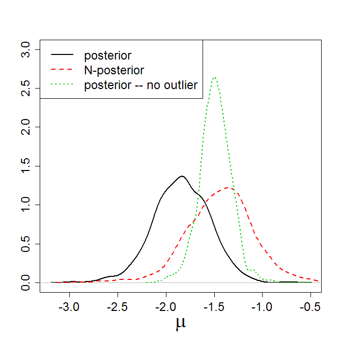
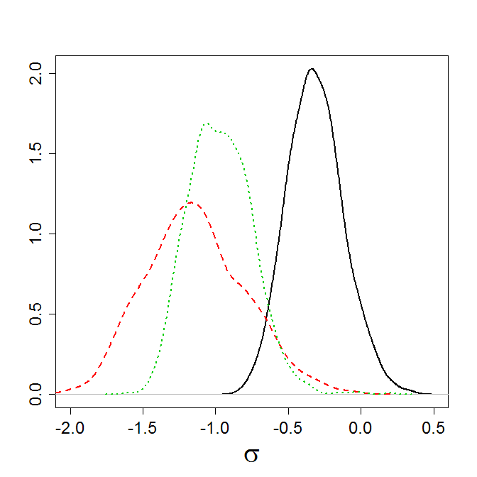
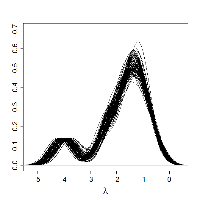
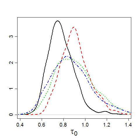
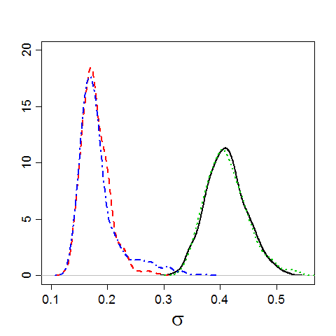
The resulting posterior distributions, given in Figure 2, indicate a substantial difference between the two posteriors, with the N-posterior having higher mean and smaller variance. This suggests some outlier contamination and a plot of a sample of densities on the right of Figure 2 suggests a lower-outlier with around -4. In fact, this corresponds to observation 5 which had unusually high efficacy in this horse. Removing the outlier results in good agreement between the posterior and the N-posterior. We note that, as also observed in Stigler (1973), trimming observations in this manner, unless done carefully, may not yield accurate credible intervals.
 |
 |
 |
8.2 Class Survey Data
Our second data set are from an in-class survey in an introductory statistics course held at Cornell University in 2009. Students were asked to specify their expected income at ages 35, 45, 55 and 65. Responses from 10 American-born and 10 foreign-born students in the class are used as data in this example; the data are presented and plotted in Online Appendix F. Our object is to examine the expected rate of increase in income and any differences in this rate or in the over-all salary level between American and foreign students. From the plot of these data in Figure 7 in Online Appendix F some potential outliers in both over-all level of expected income and in specific deviations from income trend are evident.
This framework leads to a longitudinal data model. We begin with a random intercept model
| (32) |
where is log income for the th student in group (American () or foreign ()) at age . We extend to this the distributional assumptions
leading to a complete data log likelihood given up to a constant by
| (33) |
to which we attach Gaussian priors centered at zero with standard deviations 150 and 0.5 for the and respectively and Gamma priors with shape parameter 3 and scale 0.5 and 0.05 for and . These are chosen to correspond to the approximate orders of magnitude observed in the maximum likelihood estimates of the , and residuals.
As in Section 7 we can robustify this likelihood in two different ways: either against the distributional assumptions on the or on the . In the latter case we form the density estimate
and replace the second term in (33) with . Here we have used
as an argument to to indicate its dependence on the estimated parameters. We have chosen to combine the and the together in order to obtain the best estimate of , rather than using a sum of disparities, one for American and one for foreign students.
To robustify the residual distribution, we observe that we cannot replace the first term with a single disparity based on the density of the combined since the cannot be identified marginally. Instead, we estimate a density at each :
and replace the first term with . This is the conditional form of the disparity. Note that this reduces us to four points for each density estimate; the limit of what could reasonably be employed. Naturally, both replacements can be made.
Throughout our analysis, we used Hellinger distance as a disparity; we also centered the , resulting in representing the expected salary of student at age 50. Bandwidths were fixed within a Metropolis sampling procedures. These were chosen by estimating the and via least squares, and using these to estimate residuals and all other parameters:
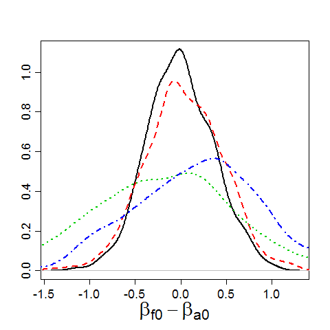
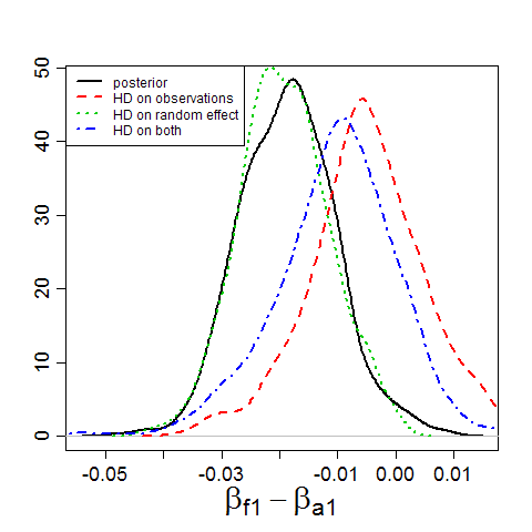
The bandwidth selector in Sheather and Jones (1991) was applied to the to obtain a bandwidth for . The bandwidth for was chosen as the average of the bandwidths selected for the for each and . For each analysis, a Metropolis algorithm was run for 200,000 steps and every 100th sample was taken from the second half of the resulting Markov chain. The results of this analysis can be seen in Figure 3. Here we have plotted only the differences and along with the variance components. We observe that for posteriors that have not robustified the random effect distribution, there appears to be a significant difference in the rate of increase in income ( for both posterior and replacing the observation likelihood with Hellinger distance), however when the random effect likelihood is replaced with Hellinger distance, the difference is no longer significant ( in both cases). We also observe that the estimated observation variance for the model is significantly reduced for posteriors in which the observation likelihood is replaced by Hellinger distance, but that uncertainty in the difference is increased.
Investigating these differences, there were two foreign students who’s over-all expected rate of increase is negative and separated from the least-squares slopes for all the other students. Removing these students increased the posterior probability of to 0.11 and decreased the estimate of from 0.4 to 0.3. Removing the evident high outlier with a considerable departure from trend at age 45 in Figure 7 in Online Appendix F further reduced the EAP of to 0.185, in the same range as those obtained from robustifying the observation distribution.
Further model exploration is possible. Online Appendix F.1 explores the use of a random slope model with additional modeling techniques, where a distinction in average slope between American and foreign students does not appear significant when the slope distribution is robustified via Hellinger distance.
 |
 |
 |
 |
9 Conclusions
This paper combines disparity methods with Bayesian analysis to provide robust and efficient inference across a broad spectrum of models. In particular, these methods allow the robustification of any portion of a model for which the likelihood may be written as a product of distributions for i.i.d. random variables. This can be done without the need to modify either the assumed data-generating distribution or the prior. In our experience, Metropolis algorithms developed for the parametric model can be used directly to evaluate the D-posterior and generally incur a modest increase in the acceptance rate and computational cost. Our use of Metropolis algorithms in this context is deliberately naive in order to demonstrate the immediate applicability of our methods in combination with existing computational tools. We expect that a careful study of the properties of these methods will yield considerable improvements in both computational and sampling efficiency.
The methods in this paper can be employed as a tool for model diagnostics; differences in results by an application of posterior and D-posterior can indicate problematic components of a hierarchical model. Further, estimated densities can indicate how the current model may be improved by, for example, the addition of mixture components. However, the D-posterior can also be used directly to provide robust inference in an automated form.
Our mathematical results are given solely for i.i.d. data; ideas from Hooker and Vidyashankar (2010a) can be used to extend these to the regression framework. Our proposal of hierarchical models remains under mathematical investigation, but we expect that similar results can be established in this case. The methodology can also be applied within a frequentist context to define an alternative marginal likelihood for random effects models, although the numerical estimation of such models is likely to be problematic. Within this context, the choice of bandwidth can become difficult. We have employed initial least-squares estimates above, but robust estimators could also be used instead. Empirically, we have found our results to be relatively insensitive to the choice of bandwidth.
An opportunity for further development of the proposed methodology lies in removing the boundedness of many disparities in common use. These yield EDAP estimates with finite-sample breakdown points of 1, indicating hyper-insensitivity to outliers. Theoretically, some form of boundedness in has been used within proofs of the robustness of minimum disparity estimators. However, transformations of can yield non-bounded replacements for the log likelihood which retain both robustness and efficiency properties and this suggests an investigation of the relationship between appropriate transformations and the structure of the parameter space .
The use of a kernel density estimate may also be regarded as inconsistent with a Bayesian context and it may be desirable to employ non-parametric Bayesian density estimates as an alternative. Results for disparity estimation are dependent on properties of kernel density estimates and this extension will require significant mathematical development.
There is considerable scope to extend these methods to further problems. Robustification of the innovation distribution in time-series models, for example, can be readily carried though through disparities and the hierarchical approach will extend this to either the observation or the innovation process in state-space models. The extension to continuous-time models such as stochastic differential equations, however, remains an open and interesting problem. More challenging questions arise in spatial statistics in which dependence decays over some domain and where a collection of i.i.d. random variables may not be available. There are also open questions in the application of these techniques to non-parametric smoothing, and in functional data analysis.
Acknowledgements
Giles Hooker’s research was supported by NSF grant DEB-0813734 and the Cornell University Agricultural Experiment Station federal formula funds Project No. 150446. Anand Vidyashankar’s research was supported in part by a grant from NSF DMS 000-03-07057 and also by grants from the NDCHealth Corporation.
References
- (1)
- Albert (2008) Albert, J. (2008). LearnBayes: Functions for Learning Bayesian Inference. R package version 2.0.
- Albert (2009) Albert, J. (2009). Bayesian Computation with R. New York: Springer.
- Andrade and O’Hagan (2006) Andrade, J. A. A. and A. O’Hagan (2006). Bayesian robustness modeling using regularly varying distributions. Bayesian Analysis 1(1), 169–188.
- Basu et al. (1997) Basu, A., S. Sarkar, and A. N. Vidyashankar (1997). Minimum negative exponential disparity estimation in parametric models. Journal of Statistical Planning and Inference 58, 349–370.
- Beran (1977) Beran, R. (1977). Minimum Hellinger distance estimates for parametric models. Annals of Statistics 5, 445–463.
- Berger (1994) Berger, J. O. (1994). An overview of robust Bayesian analysis. TEST 3, 5–124.
- Cheng and Vidyashankar (2006) Cheng, A.-L. and A. N. Vidyashankar (2006). Minimum Hellinger distance estimation for randomized play the winner design. Journal of Statistical Planning and Inference 136, 1875–1910.
- Choy and Smith (1997) Choy, S. T. B. and A. F. M. Smith (1997). On robust analysis of a normal location parameter. Journal of the Royal Statistical Society B 59, 463–474.
- Dawid (1973) Dawid, A. P. (1973). Posterior expectations for large observations. Biometrika 60, 664–667.
- Desgagnè and Angers (2007) Desgagnè, A. and J.-F. Angers (2007). Confilicting information and location parameter inference. Metron 65, 67–97.
- Devroye and Györfi (1985) Devroye, L. and G. Györfi (1985). Nonparametric Density Estimation: The L1 View. New York: Wiley.
- Dey and Birmiwal (1994) Dey, D. K. and L. R. Birmiwal (1994). Robust Bayesian analysis using divergence measures. Statistics and Probability Letters 20, 287–294.
- Engel et al. (1994) Engel, J., E. Herrmann, and T. Gasser (1994). An iterative bandwidth selector for kernel estimation of densities and their derivatives. Journal of Nonparametric Statistics 4, 21 34.
- Ghosh et al. (2006) Ghosh, J. K., M. Delampady, and T. Samanta (2006). An Introduction to Bayesian Analysis. New York: Springer.
- Hampel (1974) Hampel, F. R. (1974). The influence curve and its role in robust estimation. Journal of the american Statistics Association 69, 383–393.
- Hampel et al. (1986) Hampel, F. R., E. M. Ronchetti, P. J. Rousseeuw, and W. A. Stahel (1986). Robust statistics. Wiley Series in Probability and Mathematical Statistics: Probability and Mathematical Statistics. New York: John Wiley & Sons Inc. The approach based on influence functions.
- Hansen (2004) Hansen, B. E. (2004). Nonparametric conditional density estimation. Unpublished Manuscript: http://www.ssc.wisc.edu/~bhansen/papers/ncde.pdf.
- Hooker and Vidyashankar (2010a) Hooker, G. and A. N. Vidyashankar (2010a). Minimum disparity methods for nonlinear regression – conditional approach. Technical Report BU-1670-M, Department of Biological Statistics and Computational Biology, Cornell University.
- Hooker and Vidyashankar (2010b) Hooker, G. and A. N. Vidyashankar (2010b). Minimum disparity methods for nonlinear regression – marginal approach. in preparation.
- Huber (1981) Huber, P. (1981). Robust Statistics. New York: Wiley.
- Li and Racine (2007) Li, Q. and J. S. Racine (2007). Nonparametric Econometrics. Princeton: Princeton University Press.
- Lindsay (1994) Lindsay, B. G. (1994). Efficiency versus robustness: The case for minimum Hellinger distance and related methods. Annals of Statistics 22, 1081–1114.
- Maronna et al. (2006) Maronna, R. A., R. D. Martin, and V. J. Yohai (2006). Robust statistics. Wiley Series in Probability and Statistics. Chichester: John Wiley & Sons Ltd. Theory and methods.
- Nielsen et al. (2010) Nielsen, M., Vidyashankar, A.N., B. Hanlon, S. Petersen, and R. Kaplan (2010). Hierarchical models for evaluating anthelmintic resistance in livestock parasites using observational data from multiple farms. under reivew.
- O’Hagan (1979) O’Hagan, A. (1979). On outlier rejection phenomena in bayes inference. Journal of the Royal Statistical Society B 41, 358–367.
- O’Hagan (1990) O’Hagan, A. (1990). Outliers and credence for location parameter inference. Journal of American Statistical Association 85, 172–176.
- original by Matt Wand. R port by Brian Ripley. (2009) original by Matt Wand. R port by Brian Ripley., S. (2009). KernSmooth: Functions for kernel smoothing. R package version 2.23-3.
- Pak and Basu (1998) Pak, R. J. and A. Basu (1998). Minimum disparity estimation in linear regression models: Distribution and efficiency. Annals of the Institute of Statistical Mathematics 50, 503–521.
- Park and Basu (2004) Park, C. and A. Basu (2004). Minimum disparity estimation: Asymptotic normality and breakdown point results. Bulletin of Informatics and Cybernetics 36.
- Peng and Dey (1995) Peng, F. and D. K. Dey (1995). Bayesian analysis of outlier problems using divergence measures. Canadian Journal of Statistics 23, 199–213.
- Sheather and Jones (1991) Sheather, S. J. and M. C. Jones (1991). A reliable data-based bandwidth selection method for kernel density estimation. Journal of the Royal Statistical Society, Series B 53, 683 690.
- Silverman (1982) Silverman, B. W. (1982). Density Estimation. Chapman and Hall.
- Simpson (1987) Simpson, D. G. (1987). Minimum Hellinger distance estimation for the analysis of count data. Journal of the American statistical Association 82, 802–807.
- Simpson (1989) Simpson, D. G. (1989). Hellinger deviance test: efficiency, breakdown points and examples. Journal of the American Statistical Association 84, 107–113.
- Sollich (2002) Sollich, P. (2002). Bayesian methods for support vector machines: Evidence and predicive class probabilities. Machine Learning 46, 21–52.
- Stigler (1973) Stigler, S. M. (1973). The asymptotic distribution of the trimmed mean. Annals of Statistics 1, 427–477.
- Szpiro et al. (2010) Szpiro, A. A., K. M. Rice, and T. Lumley (2010). Model-robust regression and a Bayesian “sandwich” estimator. Annals of Applied Statistics 4, 2099–2113.
- Tamura and Boos (1986) Tamura, R. N. and D. D. Boos (1986). Minimum Hellinger distances estimation for multivariate location and and covariance. Journal of the American Statistical Association 81, 223–229.
- Zhan and Hettmansperger (2007) Zhan, X. and T. P. Hettmansperger (2007). Bayesian -estimates in two-sample location models. Comput. Statist. Data Anal. 51(10), 5077–5089.
Appendix A Proofs of Robustness
A.1 Proof of Theorem 1
Before giving the proof we remark that it follows the lines of asymptotic expansions for posterior distributions as outlined in, for example, Ghosh et al. (2006). While we have provided explicit expressions only for the first term of the expansion, further terms can be given analytically.
Proof.
Let be the MDE for the density . Using a Taylor expansion of the prior density we have:
Also, from the corresponding expansion of the disparity
yielding
where and
Here and provide constants in the Taylor of the prior and and provide the corresponding third and four-order constants in a Taylor expansion of the disparity.
In particular,for the th component of the EDAP vector we have that
| (34) |
Here the boundedness of the third derivatives of ensures the integrability of the terms. ∎
A.2 Lemmas 1 and 2
The following lemmas are needed in the proof of Theorem 2 below.
Lemma 1.
Under the conditions of Theorem 2, for any there are , and such that
| (35) |
and
| (36) |
The same results hold for given by Hellinger distance taking .
Proof.
The arguments employed here largely follow those of Park and Basu (2004, Theorem 4.1). For notational convenience throughout the following we will use and in particular we note that for , . We will also write .
For (35), define
by assumptions (12) and (14) for any we can find and large enough that and so that writing
for between and yeilds
Similarly, on taking a Taylor expansion around .
Choosing then yields the result.
For (36) we proceed in a similar manner and define
where we observe that by assumptions (12) and (13), for any and keeping bounded we can find large enough that and . Reversing the roles of and in the argument above then yields the result.
In the case of Hellinger distance, from the Cauchy-Schwartz inequality we observe that for sufficently large
and the result follows from writing Hellinger distance as .
∎
Lemma 2.
For any , if there exists such that
we can find , such that for every there exists with
| (37) |
Proof.
From Lemma 1, for any , we can find and so that for all and
and defining
Thus
and taking yields the result. ∎
A.3 Proof of Theorem 2
Proof.
We first observe that if the breakdown point of is greater than , we have
We observe that for multivariate it is sufficient to prove the result for each co-ordinate and without loss of generality we will take .
Taking and and as in Lemma 2, we now observe that we can find so that for for all such that
then
where . Since is bounded if the breakdown point is greater than , we observe that we can take
and observe that
Conversely, if the breakdown point is less than , we can find such that
and from Theorem 1 for any we can choose a subsequence such that
∎
A.4 Proof of Theorem 3
Proof.
We observe that for any finite we have
by the limiting orthogonality of and , hence we can find , so that
and and . Hence
where indicates a limit with respect to and upon observing that .
A.5 Proof of Corollary 2
Proof.
Under the assumptions, and . Now let , then for all , and therefore
Where represents expectation with respect to the prior. ∎
A.6 Proof of Theorem 4
Proof.
Since can be made to concentrate on regions where is large, we conjecture that the conditions in Theorem 4 are necessary. In fact, this requirement means that the H-posterior influence function will not be bounded for a large collection of parametric families.
Appendix B Proofs of Efficiency
B.1 Proof of Theorem 5
We begin with the following Lemma:
Proof.
We divide the integral into and :
| (39) |
and show that each vanishes in turn. First, since for some with probability 1 it follows that by Assumption A5,
This now allows us to demonstrate the convergence of the first term in (39):
| (40) |
where is a random variable and (40) converges to zero almost surely.
By Assumption A4 we can choose so that if for some positive definite matrix where indicates for all . Since with probability 1 for all sufficiently large Therefore
and the result follows from the pointwise convergence of and the dominated convergence theorem.
We can prove in an analogous manner by observing that on
and on , and
∎
Using this lemma, we prove Theorem 5.
Proof.
First, from Assumption A6, using that , and Assumption A3, it follows that
and since and Assumption A4
Now, we write that where is chosen so that . Let
From Lemma 3, it follows that from which
and
That the result holds for replaced with follows from the almost sure convergence of the latter to the former. ∎
B.2 Proof of Theorem 6
Proof.
Let , from Theorem 5
Since we have
Since , it follows that ; hence is asymptotically normal, efficient as well as robust. ∎
B.3 Efficiency Conditions for Minimum Disparity Estimators
Here we provide conditions that ensure the consistency and asymptotic normailty of the minimum-disparity estimator . There is a slight variation through the literature in conditions required for efficiency (see Beran (1977), Basu et al. (1997), Park and Basu (2004) and Cheng and Vidyashankar (2006)). The conditions given below are adapted from Cheng and Vidyashankar (2006) for the specific case of Hellinger distance. A small modification of these conditions will also provide the consistency and asymptotic normality for more general disparities under appropriate conditions on . These are in addition to conditions A2-A5.
We first require conditions on the data and the proposed parametric family:
-
(D1)
are i.i.d. with distribution given by the density function .
-
(D2)
The parameter space is locally compact.
-
(D3)
is twice continuously differentiable with respect to .
-
(D4)
is continuous and bounded.
-
(D5)
is continuous and bounded in at .
-
(D6)
is continuous and bounded in at .
-
(D7)
is continuous and bounded in at .
We also require conditions on the kernel function in the kernel density estimate and its relationship to the parametric density family:
-
(K1)
is symmetric about 0 and .
-
(K2)
The bandwidth is chosen so that , , .
-
(K3)
There is a sequence , diverging to infinity such that
-
(a)
For a random variable with density
-
(b)
-
(c)
The parametric score functions have regular central behavior relative to the bandwidth:
and
-
(d)
The score functions are smooth with respect to in an sense:
-
(a)
This statement of assumptions in particular remove the condition that has compact support, which was assumed in Beran (1977); Basu et al. (1997); Park and Basu (2004). These assumptions significantly expand the class of kernels available for use and hence expands the applicability of Theorem 5 (see Hooker and Vidyashankar (2010b) for formal details). In practice, it is numerically more stable to use a Gaussian kernel or some other distribution with support on the whole real line and we have used Gaussian kernels throughout our numerical experiments. We also follow Cheng and Vidyashankar (2006) in removing the assumption of compactness of , replacing it with local compactness plus the identifiability condition A5.
Appendix C Reducing the Kernel Density Dimension
The conditional disparity formulation outlined above requires the estimation of the density of a response conditioned on a potentially high-dimensional set of covariates; this can result in asymptotic bias and poor performance in small samples. In this section, we explore two methods for reducing the dimension of the conditioning spaces. The first is referred to as the “marginal formulation” and requires only a univariate, unconditional, density estimate. This is a Bayesian extension of the approach suggested in Hooker and Vidyashankar (2010b). It is more stable and computationally efficient than schemes based on nonparametric estimates of conditional densities. However, in a linear-Gaussian model with Gaussian covariates, it requires an external specification of variance parameters for identifiability. For this reason, we propose a two-step Bayesian estimate. The asymptotic analysis for i.i.d. data can be extended to this approach by using the technical ideas in Hooker and Vidyashankar (2010b).
The second method produces a conditional formulation that relies on the structure of a homoscedastic location-scale family and we refer to it as the “conditional-homoscedastic” approach. This method provides a full conditional estimate by replacing a non-parametric conditional density estimate with a two-step procedure as proposed in Hansen (2004). The method involves first estimating the mean function non-parametrically and then estimating a density from the resulting residuals.
C.1 Marginal Formulation
Hooker and Vidyashankar (2010b) proposed basing inference on a marginal estimation of residual density in a nonlinear regression problem. A model of the form
is assumed for independent from a scale family with mean zero and variance . is an unknown parameter vector of interest. A disparity method was proposed based on a density estimate of the residuals
yielding the kernel estimate
| (41) |
and was estimated by minimizing
where is is the
postulated density. As described above, in a Bayesian context we replace the
log likelihood by
. Here we
note that although the estimated of need not have
zero mean, it is compared to the centered density which
penalizes parameters for which the residuals are not centered.
This formulation has the advantage of only requiring the estimate of a univariate, unconditional density . This reduces the computational cost considerably as well as providing a density estimate that is more stable in small samples.
Hooker and Vidyashankar (2010b) proposed a two-step procedure to avoid identifiability problems in a frequentist context. This involves replacing by a robust external estimate . It was observed that estimates of were insensitive to the choice of . After an estimate was obtained by minimizing , an efficient estimate of was obtained by re-estimating based on a disparity for the residuals . A similar process can be undertaken here.
In a Bayesian context a plug-in estimate for also allows the use of the marginal formulation: an MCMC scheme is undertaken with the plug-in value of held fixed. A pseudo-posterior distribution for can then be obtained by plugging in an estimate for to a Disparity-Posterior for . More explicitly, the following scheme can be undertaken:
-
1.
Perform an MCMC sampling scheme for using a plug-in estimate for .
-
2.
Approximate the posterior distribution for with an MCMC scheme to sample from the D-posterior where is the EDAP estimate calculated above.
This scheme is not fully Bayesian in the sense that fixed estimators of and are used in each step above. However, we conjecture that, as in Hooker and Vidyashankar (2010b), the two-step procedure will result in statistically efficient estimates and asymptotically correct credible regions. We note that while we have discussed this formulation with respect to regression problems, it can also be employed with the plug-in procedure for random-effects models and we use this in Section 8.2, below.
The formulation presented here resembles the methods proposed in Pak and Basu (1998) based on a sum of disparities between weighted density estimates of the residuals and their expectations assuming the parametric model. For particular combinations of kernels and densities, these estimates are efficient, and the sum of disparities, appropriately scaled, should also be substitutable for the likelihood in order to achieve an alternative D-posterior.
C.2 Nonparametric Conditional Densities for Regression Models in Location-Scale Families
Under a homoscedastic location-scale model (where the errors are assumed to be i.i.d.) where is a distribution with zero mean, an alternative density estimate may be used. We first define a non-parametric estimate of the mean function
and then a non-parametric estimate of the residual density
We then consider the disparity between the proposed and :
As before, can be substituted for the log likelihood in an MCMC scheme.
Hansen (2004) remarks that in the case of a homoscedastic conditional density, has smaller bias than . This formulation does not avoid the need to estimate the high-dimensional function . However, the shift in mean does allow the method to escape the identification problems of the marginal formulation while retaining some of its stabilization.
Online Appendix E.2 gives details of a simulation study of both conditional formulations and the marginal formulation above for a regression problem with a three-dimensional covariate. All disparity-based methods perform similarly to using the posterior with the exception of the conditional form in Section 6 when Hellinger distance is used which demonstrates a substantial increase in variance. We speculate that this is due to the sparsity of the data in high dimensions creating inliers; negative exponential disparity is less sensitive to this problem (Basu et al., 1997).
Appendix D Computational Considerations and Implementation
Our experience is that the computational cost of employing Disparity-based methods as proposed above is comparable to employing an MCMC scheme for the equivalent likelihood and generally requires an increase in computation time by a factor of between 2 and 10. Further, the comparative advantage of employing estimates (5) versus (6) depends on the context that is used.
Formally, we assume Monte Carlo samples is (5) and Gauss-Hermite quadrature points in (6) where typically . In this case, the cost of evaluating in (5) is , but this may be pre-computed before employing MCMC, and the cost of evaluating (5) for a new value of is . In comparison, the use of (6) requires the evaluation of at each iteration at a each evaluation.
Within the context of conditional disparity metrics, we assume Monte Carlo points used for each in the equivalent verion of (5) for (26) and note that in this context can be reduced due to the additional averaging over the . The cost of evaluating from (25) for all and is for (5) and for (6). Here again the computation can be carried out before MCMC is employed for (5), requiring operations. In (6) the denominator of (25) can be pre-computed, reducing the computational cost of each iteration to ; however, in this case we will not necessarily expect . Similar calculations apply to estimates based on .
For marginal disparities in (41) changes for each , requiring calculations to evaluate (6). Successful use of (5) would require the to vary smoothly with and would also require the re-evaluation of at a cost of each iteration. Within the context of hierarchical models above, varies with latent variables and this the use of (5) will generally be more computationally efficient. The cost of evaluating the likelihood is always .
While these calculations provide general guidelines to computational costs, the relative efficiency of (5) and (6) strongly depends on the implementation of the procedure. Our simulations have been carried out in the R programming environment where we have found (5) to be computationally cheaper anywhere it can be employed. However, this will be platform-dependent – changing with what routines are given in pre-compiled code, for example – and will also depend strongly on the details of our implementation.
Appendix E Simulation Studies
While we have established attractive asymptotic properties for these estimators their finite sample properties remain an important source of investigation. Since these estimates are based on nonparametric density estimation, we may suspect that they require large sample sizes before their asymptotic properties become apparent. In fact, our studies below demonstrate good performance even for small sample sizes.
E.1 Gaussian and exponential-Gamma Distributions – The i.i.d. Case
We undertook a simulation study for the normal mean example in Figure 1 to examine the efficiency and robustness of Hellinger and Negative-Exponential posterior samples. 1,000 sample data sets of size 20 from a population were generated. For each sample data set, a random walk Metropolis algorithm was run for 20,000 steps using a proposal distribution and a prior, placing the true mean one prior standard deviation above the prior mean. The kernel bandwidth was selected by the bandwidth selection in Sheather and Jones (1991). H- and N-posteriors were easily calculated by combining the KernSmooth (original by Matt Wand. R port by Brian Ripley., 2009) and LearnBayes (Albert, 2008) packages in R. Expected a posteriori estimates for the sample mean were obtained along with 95% credible intervals from every second sample in the second half of the MCMC chain. Outlier contamination was investigated by reducing the last one, two or five elements in the data set by 3, 5 or 10. This choice was made so that both outliers and prior influence the EDAP in the same direction. The analytic posterior without the outliers is normal with mean 4.99 (equivalently, bias of -0.01) and standard deviation 0.223. The results of this simulation are summarized in Table 3. As can be expected, the standard Bayesian posterior suffers from sensitivity to large negative values whereas the disparity-based methods remain nearly unchanged. Near-outliers at the smaller value of -3 resulted in similar biases across all methods. A comparison of CPU time indicates that the use of disparity methods required a little more than twice the computational effort as compared to using the likelihood within an MCMC method.
In order to provide a comparison with classical robust methods, we conducted a comparison with an estimate based on a Huberized mean. Table 4 provides the results of these estimates using the Huber loss as a log likelihood within an MCMC scheme and by the minimizer of the Huber loss. In both cases, we tried cut-points between quadratic and linear costs at the normal 0.8 and 0.99 critical values. We also considered replacing the log likelihood within the MCMC scheme with a loss corresponding to Tukey’s biweight function with cut point 4.685; this has the appeal of being similar to disparity methods in both having a re-descending influence function and tails of the likelihood that do not go to zero at infinity. We notice here that Huberized methods with cut point at the 0.8 critical value and Tukey’s biweight method both showed noticeable increases in standard deviation compared to Hellinger methods and the likelihood when no outliers were added to the data. The negative exponential disparity had a similar increase in variance in this case which we speculate is due to having relatively heavier tails than Hellinger distance and therefore greater influence from the prior (the maximal value of NED is where as that of 2HD is 4). While Huber both methods exhibited less bias due to outliers than the likelihood, the bias still grew substantially with large outliers. By contrast, both biweight and disparity methods demonstrate redescending influence as outliers are placed at more extreme values, but we observe that the biweight estimates were more strongly affected for larger numbers of contaminated observations. Disparity-based methods had credible intervals between 5% and 15% wider than those based on the likelihood, but these were smaller than those for Huberized and biweight methods when a prior was employed. The computing times for MCMC methods using Huber and biweight likelihoods are somewhat greater than for the use of the true likelihood, although computing the minimizing value is unsurprisingly faster.
The problem of estimating a Gaussian mean is made relatively straightforward by the symmetry of the distribution. We therefore conducted a further study, estimating both shape and scale parameters in an exponential-gamma distribution (ie, has a distribution, and the domain of the distribution is the whole real line). In this case, the shape parameter was chosen at 5 and the scale parameter at 0.25 and these were given priors with degrees of freedom 3 and 0.3 respectively. 5,000 data sets were simulated of 20 points each and the D-posteriors were calculated as above both with and without an outlier placed at ln(20). For this chain a random walk Metropolis algorithm was again conducted with the random walk on the log shape and log scale parameters again using the LearnBayes package. Table 5 reports the tabulated results. We note in particular that the efficiency of the H-posterior has been considerably reduced, as have its coverage properties; additionally two simulation runs were removed due to poor convergence. This is explained as being due to the inlier effect; the skewness of the gamma distribution produces density estimates that tend to have “holes” and the Hellinger disparity is sensitive to these; an example is give in Figure 4. By contrast, the negative exponential disparity is much less sensitive.
No Outliers
| Bias | SD | Coverage | Length | CPU Time | |
|---|---|---|---|---|---|
| Posterior | -0.015 | 0.222 | 0.956 | 0.873 | 3.393 |
| Hellinger | -0.015 | 0.225 | 0.954 | 0.920 | 7.669 |
| Negative Exponential | -0.018 | 0.229 | 0.973 | 1.022 | 7.731 |
Outliers
| 1 Outlier | 2 Outliers | 5 Outliers | ||||||||
|---|---|---|---|---|---|---|---|---|---|---|
| Loc | Bias | SD | Coverage | Bias | SD | Coverage | Bias | SD | Coverage | |
| Posterior | -3 | -0.164 | 0.219 | 0.883 | -0.300 | 0.206 | 0.722 | -0.637 | 0.182 | 0.100 |
| -5 | -0.264 | 0.219 | 0.778 | -0.490 | 0.206 | 0.375 | -1.053 | 0.182 | 0.001 | |
| -10 | -0.513 | 0.219 | 0.360 | -0.965 | 0.207 | 0.004 | -2.093 | 0.182 | 0.000 | |
| HD | -3 | -0.109 | 0.246 | 0.920 | -0.194 | 0.275 | 0.859 | -0.237 | 0.299 | 0.770 |
| -5 | -0.027 | 0.238 | 0.942 | -0.040 | 0.257 | 0.928 | -0.024 | 0.305 | 0.865 | |
| -10 | -0.014 | 0.234 | 0.948 | -0.019 | 0.249 | 0.935 | 0.018 | 0.286 | 0.883 | |
| NED | -3 | -0.080 | 0.256 | 0.959 | -0.133 | 0.279 | 0.933 | -0.166 | 0.308 | 0.893 |
| -5 | -0.020 | 0.238 | 0.977 | -0.025 | 0.243 | 0.968 | -0.015 | 0.264 | 0.948 | |
| -10 | -0.017 | 0.237 | 0.973 | -0.020 | 0.241 | 0.970 | -0.007 | 0.260 | 0.952 | |
No Outliers
| Bias | SD | Coverage | Length | CPU Time | |
| Bayes 80 | -0.017 | 0.229 | 0.973 | 0.978 | 5.337 |
| Bayes 99 | -0.015 | 0.223 | 0.956 | 0.877 | 4.962 |
| Freq 80 | -0.004 | 0.229 | 0.948 | 0.894 | 0.002 |
| Freq 99 | -0.004 | 0.223 | 0.960 | 0.894 | 0.001 |
| Biweight | -0.017 | 0.228 | 0.977 | 1.007 | 3.523 |
Outliers
| 1 Outlier | 2 Outliers | 5 Outliers | ||||||||
|---|---|---|---|---|---|---|---|---|---|---|
| Loc | Bias | SD | Coverage | Bias | SD | Coverage | Bias | SD | Coverage | |
| Bayes | 3 | -0.102 | 0.237 | 0.948 | -0.188 | 0.235 | 0.904 | -0.450 | 0.241 | 0.584 |
| 80 | 5 | -0.101 | 0.237 | 0.950 | -0.188 | 0.235 | 0.907 | -0.451 | 0.241 | 0.582 |
| 10 | -0.101 | 0.237 | 0.946 | -0.188 | 0.236 | 0.907 | -0.450 | 0.241 | 0.574 | |
| Bayes | 3 | -0.149 | 0.228 | 0.894 | -0.282 | 0.221 | 0.757 | -0.635 | 0.192 | 0.153 |
| 99 | 5 | -0.151 | 0.231 | 0.893 | -0.290 | 0.228 | 0.754 | -0.704 | 0.231 | 0.147 |
| 10 | -0.151 | 0.231 | 0.887 | -0.290 | 0.228 | 0.760 | -0.704 | 0.231 | 0.148 | |
| Freq | 3 | -0.087 | 0.238 | 0.922 | -0.172 | 0.236 | 0.872 | -0.429 | 0.242 | 0.454 |
| 80 | 5 | -0.087 | 0.238 | 0.922 | -0.172 | 0.236 | 0.872 | -0.429 | 0.242 | 0.454 |
| 10 | -0.087 | 0.238 | 0.922 | -0.172 | 0.236 | 0.872 | -0.429 | 0.242 | 0.454 | |
| Freq | 3 | -0.140 | 0.230 | 0.898 | -0.275 | 0.223 | 0.753 | -0.633 | 0.188 | 0.115 |
| 99 | 5 | -0.140 | 0.231 | 0.897 | -0.279 | 0.229 | 0.751 | -0.693 | 0.231 | 0.115 |
| 10 | -0.140 | 0.231 | 0.897 | -0.279 | 0.229 | 0.751 | -0.693 | 0.231 | 0.115 | |
| Biweight | 3 | -0.091 | 0.246 | 0.954 | -0.175 | 0.252 | 0.915 | -0.443 | 0.275 | 0.645 |
| 5 | -0.018 | 0.237 | 0.974 | -0.019 | 0.236 | 0.972 | -0.022 | 0.243 | 0.967 | |
| 10 | -0.017 | 0.236 | 0.977 | -0.018 | 0.234 | 0.971 | -0.018 | 0.236 | 0.969 | |
| No Outliers | ||||||
|---|---|---|---|---|---|---|
| Shape | Scale | |||||
| Bias | Variance | Coverage | Bias | Variance | Coverage | |
| Posterior | -0.088 | 0.571 | 0.9516 | 0.004 | 0.0005 | 0.9562 |
| Hellinger | -0.081 | 1.005 | 0.850 | 0.010 | 0.0011 | 0.839 |
| Negative Exponential | -0.182 | 0.739 | 0.9436 | 0.008 | 0.0007 | 0.9556 |
| Outlier at 20 | ||||||
| Shape | Scale | |||||
| Bias | Variance | Coverage | Bias | Variance | Coverage | |
| Posterior | -3.068 | 0.001 | 0 | 0.988 | 0.00006 | 0 |
| Hellinger | -0.013 | 1.046 | 0.8508 | 0.010 | 0.0011 | 0.8440 |
| Negative Exponential | -0.210 | 0.725 | 0.9496 | 0.010 | 0.0008 | 0.9586 |
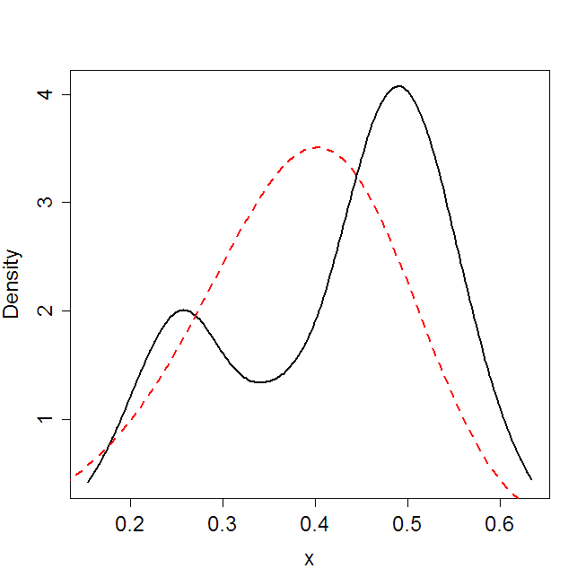
E.2 Linear Regression Models
Figure 5 provides example D-posterior distributions of all regression disparities described in Sections 6 and C along with the posterior for an example 3-dimensional linear regression based on 30 points. Both Hellinger and negative exponential disparities were used. Covariates were generated from a standard normal distribution with errors also generated from a standard normal distribution. The likelihood is noticeably more concentrated than the disparity-based posteriors, but all exhibit broadly similar shapes.
We have supplemented this experiment with a simulation. 1,000 data sets were simulated from a linear regression model on three covariates. The covariates were chosen from a three dimensional normal distribution with unit marginal variances and correlation 0.5 between each pair of covariates. These were held fixed across all simulations. The parameters in the model were chosen as . Bandwidths were chosen using the criterion in Sheather and Jones (1991) based on the observed covariates and maximum likelihood estimates of the residuals. Both Hellinger distance and negative exponential disparity were considered, and the conditional formulation, marginal formulation and conditional-homoscedastic form were used to estimate the five parameters in the model. Additionally, we obtained Huberized estimators by replacing the log likelihood with a Huber loss function and minimizing the Huber loss function. This resulted in seven estimators including a Gaussian posterior. For each estimate a random-walk Metropolis algorithm was run for 10,000 steps and EDAP estimates were calculated from every fifth sample in the second half of the chain. The results from this study are given in Table 6. Here we observe good agreement between all disparity-based methods and the likelihood. The choice between these will therefore depend on the amount of data available and the dimension of the covariate space. Computing time is reported in this simulation as well where disparity methods increase computing costs by a factor of between 3 and 5 while the use of a Huber loss within MCMC corresponds to about a 1.5 factor increase in cost. We note, however, that relative computing costs in interpreted languages such as R are strongly dependent on the details of implementation.
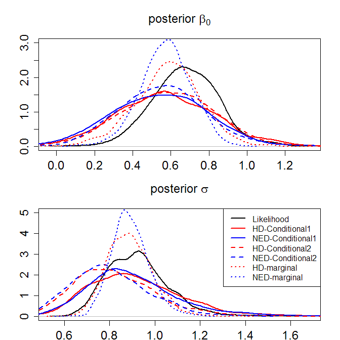 |
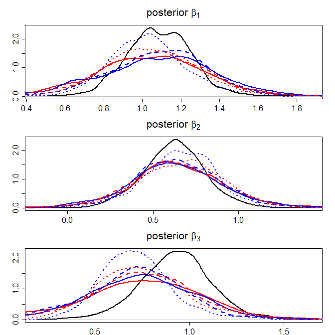 |
| Sigma | beta 0 | beta 1 | beta 2 | beta 3 | time | |
| Likelihood | 1.030 (0.137) | 0.996 (0.186) | 0.993 (0.194) | 0.998 (0.217) | 1.006 (0.301) | 20.251 |
| HD | 0.974 (0.154) | 1.000 (0.213) | 0.993 (0.204) | 0.994 (0.239) | 0.980 (0.301) | 62.315 |
| NED | 0.926 (0.136) | 0.997 (0.201) | 0.994 (0.206) | 1.001 (0.224) | 0.964 (0.294) | 70.812 |
| HD hom | 0.881 (0.181) | 0.995 (0.338) | 0.987 (0.198) | 0.995 (0.217) | 0.980 (0.296) | 62.184 |
| NED hom | 0.829 (0.157) | 0.993 (0.235) | 0.988 (0.211) | 0.996 (0.228) | 0.974 (0.313) | 70.649 |
| HD marg | 1.062 (0.133) | 0.997 (0.193) | 0.994 (0.203) | 0.997 (0.225) | 1.003 (0.309) | 102.959 |
| NED marg | 1.087 (0.137) | 1.000 (0.199) | 0.994 (0.210) | 0.998 (0.232) | 1.005 (0.321) | 102.966 |
| Huber EAP | 0.878 (0.123) | 0.998 (0.192) | 0.994 (0.198) | 1.000 (0.221) | 1.005 (0.306) | 34.861 |
| Huber min | 0.919 (0.207) | 0.999 (0.191) | 0.995 (0.198) | 1.000 (0.222) | 1.006 (0.307) | 0.013 |
E.3 One-Way Random Effects Models
Figure 6 demonstrates the differences resulting from robustifying different distributional assumptions in the one-way random effects model described in Section 7. We simulated a set of five groups of twenty observations. Each group had variance 0.2 with a mean drawn from a population. This produces a random-effects model and the goal is to estimate . The plots in Figure 6 show that the use of disparity methods in either the random effect or on the residual process or on both provide very similar distributions to the correct posterior. When an outlying group is added with mean 40, those methods that replace the random effects distribution with a disparity are unaffected while those that do not are substantially biased.
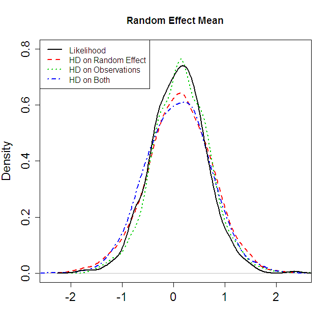 |
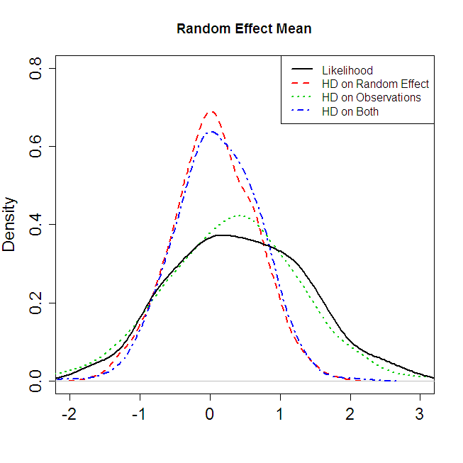 |
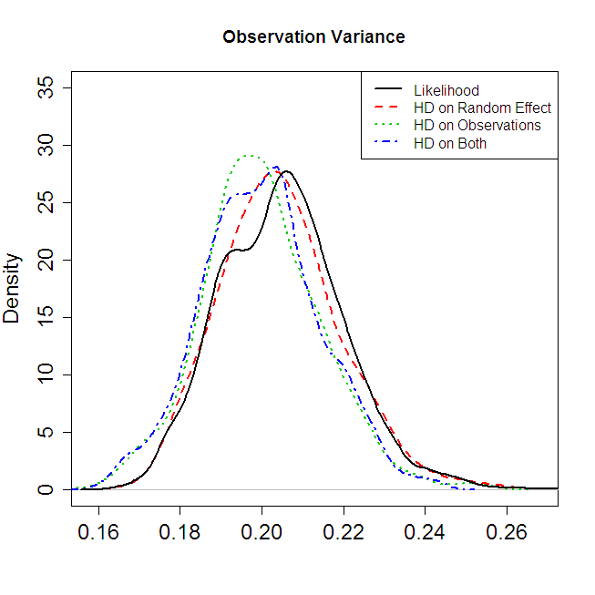 |
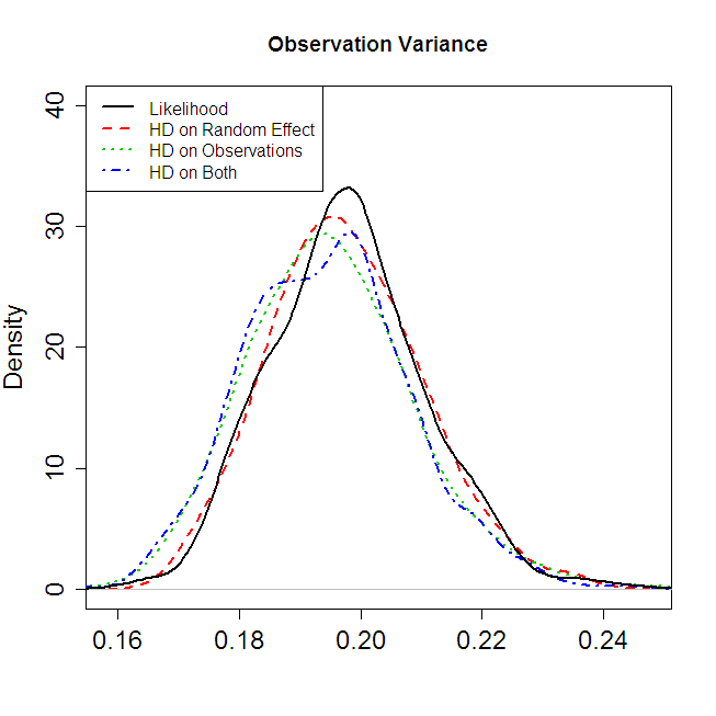 |
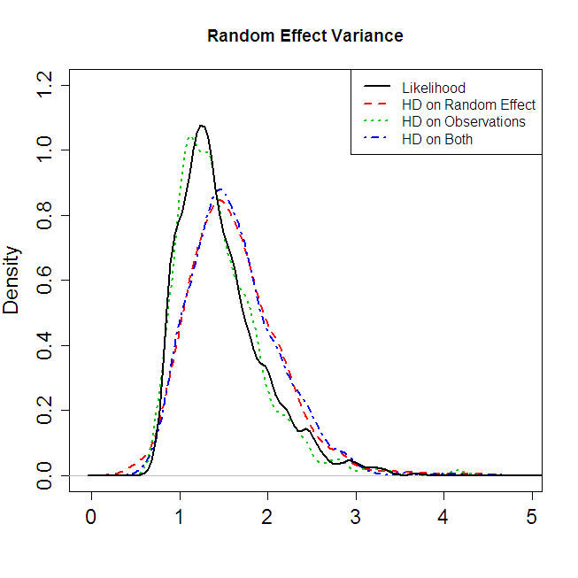 |
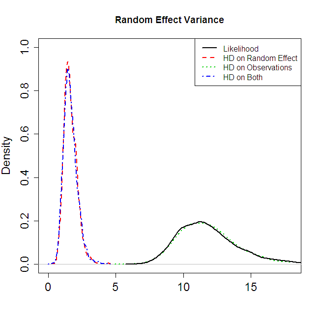 |
In order to verify the apparent success of this method, we conducted a simulation study of a one-way random effects model with ten random effects and five observations per random effect. The random effects were simulated from a standard normal distribution, while the observations were Gaussian, centered on the random effect and with standard deviation 0.2. We simulated 1,000 versions of these data. For each version a random-walk Metropolis scheme was run to sample from the posterior, the posterior with the observation likelihood replaced by H-posterior, the posterior with the random effect likelihood replaced by H-posterior and the posterior with both replacements. All MCMC schemes were run for 10,000 steps with posterior distributions calculated based on every 5th sample from the second half of the chain. We additionally added a further random effect with five observations distributed around the value 40 with standard deviation 0.2. Bandwidth parameters were chosen by the selection criterion of Sheather and Jones (1991) based on maximum-likelihood estimates of random effects and residual errors. The results of this simulation are summarized in Table 7. Here we see that the estimation of is biased downwards by the estimation of a conditional density for each random effect, based on only five observations and there is more uncertainty in the estimate of when Hellinger distance is used in place of the random effect log likelihood. The disparity-based methods otherwise perform very similarly to the true likelihood. When an outlying random effect is added, replacing the random effect likelihood with Hellinger distance robustified inference, where those posteriors without this replacement were severely biased.
| No Outliers | |||||||||
|---|---|---|---|---|---|---|---|---|---|
| sd() | coverage | sd() | coverage | sd() | coverage | ||||
| Likelihood | 0.0013 | 0.286 | 0.947 | 0.200 | 0.0230 | 0.940 | 0.979 | 0.234 | 0.919 |
| HD - obs | 0.0035 | 0.285 | 0.937 | 0.200 | 0.0231 | 0.939 | 1.070 | 0.342 | 0.900 |
| HD - rand | 0.0021 | 0.286 | 0.936 | 0.191 | 0.0259 | 0.686 | 0.982 | 0.231 | 0.928 |
| HD - both | 0.0024 | 0.291 | 0.933 | 0.191 | 0.0258 | 0.692 | 1.068 | 0.342 | 0.899 |
| Outlying Random Effect | |||||||||
| sd() | coverage | sd() | coverage | sd() | coverage | ||||
| Likelihood | 0.365 | 0.197 | 1.000 | 0.200 | 0.0222 | 0.930 | 10.11 | 0.163 | 0.000 |
| HD - obs | 0.002 | 0.288 | 0.926 | 0.200 | 0.0223 | 0.922 | 1.088 | 0.389 | 0.887 |
| HD - rand | 0.353 | 0.252 | 1.000 | 0.191 | 0.0249 | 0.684 | 10.13 | 0.196 | 0.000 |
| HD - both | 0.002 | 0.295 | 0.917 | 0.191 | 0.0249 | 0.674 | 1.066 | 0.325 | 0.885 |
Appendix F Data
Table 8 provides the values of the parasitology data set used in Section 8.1. The data used for the class survey data in Section 8.2 are provided in Table 9; they are graphed in Figure 7.
| Horse | 1 | 2 | 3 | 4 | 5 | 6 | 7 |
|---|---|---|---|---|---|---|---|
| Pre-treatment | 2440 | 1000 | 1900 | 1820 | 3260 | 300 | 660 |
| Post-treatment | 580 | 320 | 400 | 160 | 60 | 40 | 120 |
| Status | 35 | 45 | 55 | 65 |
|---|---|---|---|---|
| a | 11.51293 | 11.775290 | 11.98293 | 12.10071 |
| a | 11.91839 | 12.206073 | 12.61154 | 12.20607 |
| a | 11.69525 | 12.100712 | 12.42922 | 12.42922 |
| a | 11.69525 | 12.100712 | 12.38839 | 12.79386 |
| a | 10.71442 | 10.819778 | 10.81978 | 10.81978 |
| a | 11.15625 | 11.512925 | 11.84940 | 11.98293 |
| a | 10.51867 | 10.596635 | 10.71442 | 11.00210 |
| a | 12.20607 | 12.206073 | 12.20607 | 12.20607 |
| a | 9.21034 | 9.903488 | 10.12663 | 10.30895 |
| a | 10.59663 | 11.002100 | 11.28978 | 11.40756 |
| a | 14.22098 | 12.100712 | 14.91412 | 15.60727 |
| f | 11.51293 | 11.918391 | 11.51293 | 10.81978 |
| f | 11.00210 | 11.002100 | 11.15625 | 11.15625 |
| f | 11.91839 | 12.206073 | 12.42922 | 12.42922 |
| f | 11.40756 | 11.695247 | 11.73607 | 11.77529 |
| f | 11.91839 | 13.122363 | 13.30468 | 13.30468 |
| f | 11.51293 | 11.695247 | 11.91839 | 12.20607 |
| f | 11.15625 | 11.512925 | 11.51293 | 11.69525 |
| f | 12.20607 | 12.611538 | 12.76569 | 11.00210 |
| f | 10.81978 | 11.002100 | 11.00210 | 11.00210 |
| f | 10.46310 | 11.002100 | 11.08214 | 11.08214 |
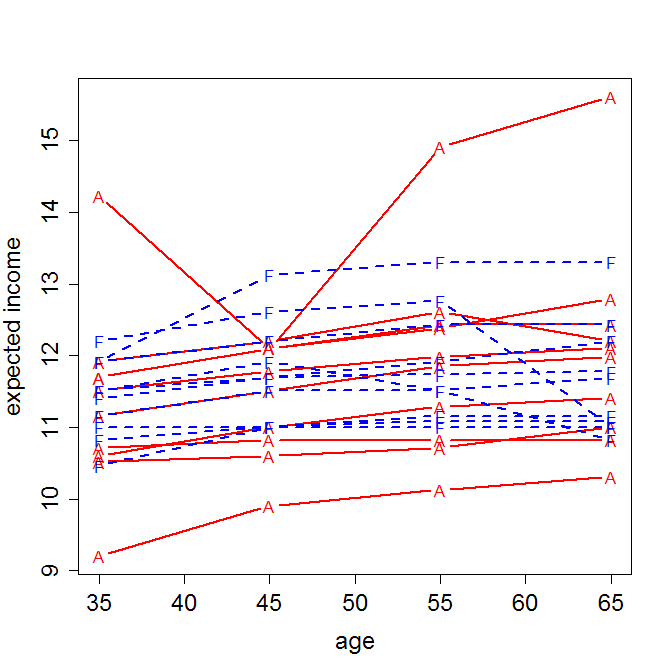
F.1 Random Slope Models for Class Survey Data
A further model exploration of the class survey data allows a random slope for each student in addition to the random offset. The model now becomes
| (42) |
with additional distributional assumptions
and an additional term
added to (33). Here, this term can be robustified in a similar manner to the robustification of the . However, we note that a robustification of the error terms would require the estimation of a conditional density for each – based on only four data points. We viewed this as being too little to achieve reasonable results and therefore employed the marginal formulation described in Section C. Specifically, we first obtained residuals for the random slope model from the maximum likelihood estimates for each subject-specific effect and estimated
Following this, we estimated a combined density for all residuals, conditional on the random effects
and replaced the first term in (33) with . Following the estimation of all other parameters, we obtained new residuals where the and are the EDAP estimators. We then re estimated based on its H-posterior using the as data. In this particular case a large number of outliers from a concentrated peak (see Figure 8) meant that the use of Gauss-Hermite quadrature in the evaluation of
suffered from large numerical errors and we therefore employed a Monte Carlo integral based on 400 data points drawn from instead, using the estimate (5). To estimate both and the other parameters we used a Metropolis random walk algorithm which was again run for 200,000 iterations with estimates based on every 100th sample in the second half of the chain.
Some results from this analysis are displayed in Figure 8. The residual distribution of the show a very strong peak and a number of isolated outliers. The estimated standard deviation of the residual distribution is therefore very different between those methods that are robust to outliers and those that are not; the mean posterior was increased by a factor of four between those methods using a Hellinger disparity and those using the random effect log likelihood. The random slope variance was estimated to be small by all methods – we speculate that the distinction between random effect log likelihoods and Hellinger methods is bias due to bandwidth size – but this was not enough to overcome the differences between the methods concerning the distinction between and .
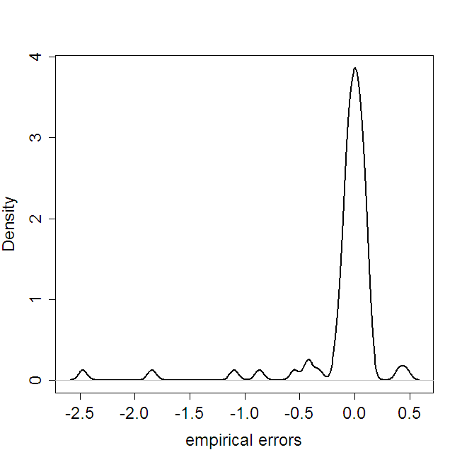 |
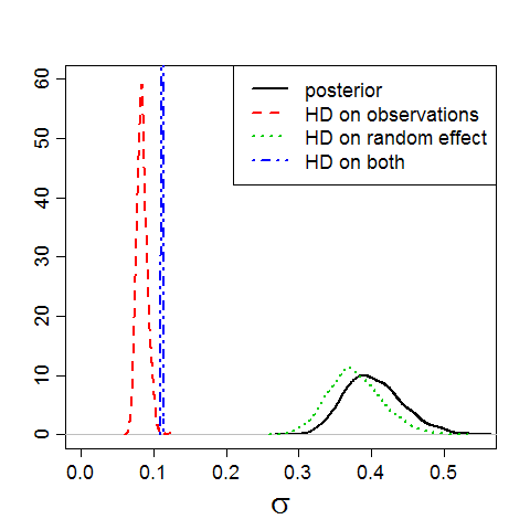 |
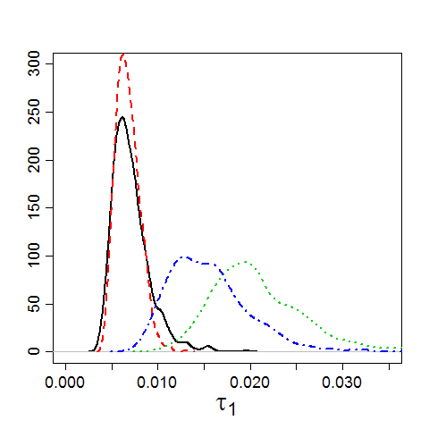 |
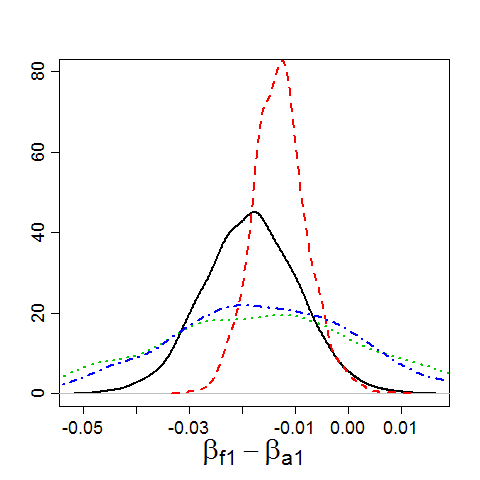 |