An Introduction to the Theory of Tachyons

Abstract

The theory of relativity, which was proposed in the beginning of the 20th century, applies to particles and frames of reference whose velocity is less than the velocity of light. In this paper we shall show how this theory can be extended to particles and frames of reference which move faster than light.

1 The need for a theory of tachyons

Scientists at the European Organization for Nuclear Research (CERN) recently reported the results of an experiment [1] on which faster than light neutrinos were probably detected. Coincidentally, about a week before the divulgation of this result, I was fortunate to present at the 7th UFSCar Physics Week [2] a lecture precisely on the subject of tachyons (the name given in theoretical physics to faster than light particles). Students and Professors were very interested on this lecture, specially after the news discussed above. I have been encouraged since then to write a paper about the ideas presented on that occasion, which constitute the present text.

Regardless of the results presented in [1] are correct or not, we point out that there are other experimental evidences for existence of superluminal phenomena in nature [3]. Moreover, the theory of tachyons could provide a better understanding of the theory of relativity as well as some issues of quantum mechanics and we believe that these arguments are enough for one to try to formulate an extended theory of relativity, which applies to faster than light phenomena, particles and reference frames. Attempts to extend the theory of relativity have been, of course, proposed by many scientists, although the original sources are not easily accessible (in fact, only recently I had knew about these works). Among the formulations proposed, we highlight the works of Recami and collaborators [4], whose results coincide mostly with those who will be presented here. Reference [4] is a review on the subject, where the interested reader will find a vast amount of references and may also get more details about the theory, besides topics which will not be discussed here (e.g., the tachyon electrodynamics).

For an extended theory of relativity, we mean a theory which applies to particles and frames of reference moving with a velocity greater than $c$ – the speed of light in vacuum –, and also to particles and reference frames “moving” back in time. In particular it is necessary to extend the Lorentz transformations for such frames. Although we have no problem at all to extend the Lorentz transformations in a two-dimensional universe, $(x,t)$, we meet with certain difficulties when we try to extend them in a universe of four dimensions, $(x,y,z,t)$. The reasons why this happens will be commented in section 10. Finally, in section 11 we shall show that in a six-dimensional world (3 space-like dimensions and other 3 time-like ones), we can make those difficulties to disappear and therefore that becomes possible, in this six-dimensional universe, to extend the Lorentz transformations in agreement with the usual principles of relativity.

One of the reasons which makes the theory of tachyons almost unknown is the (equivocated) belief that the theory of relativity forbids the existence of faster than light particles, and that the light speed represents an upper limit for the propagation of any phenomena in nature. The argument commonly used to prove this statement is, as stated by the theory of relativity, that no particle whatsoever can be accelerated to reach or to exceed the speed of light, since this would require spending an infinite amount of energy. This is not wrong, but is also not completely correct. Indeed, this argument ignores the possibility of these particles have been created at the same time as the Big-Bang. In this way nobody had to speed them up – they just were born already with a greater than light speed.

Moreover, we can not rule out the possibility that such particles might be created through some quantum process, analogous for instance to the process of creation of particle-antiparticle pairs.

Finally, if we associate a complete isotropy and homogeneity to the space-time, then it follows that none of their directions should be privileged with respect to the others and thus the existence of faster than light particles would naturally be expected instead of be regarded as surprising. It is not the possibility of existence of tachyons which requires explanation, on the contrary, an explanation must to be given in the case of these particles do not exist.

2 On the space-time structure

As is known, the formulation of the theory of relativity was due to the efforts of several scientists (e.g., Lorentz, Poincaré, Einstein, Minkowski etc.). The geometric description of the relativity theory – the so-called space-time theory – in its turn, was first proposed by Poincaré [5] in 1905 and after independently by Minkowski [6] in 1909, where a more accessible and detailed presentation of the subject was presented.

This geometric description, which contains the very essence of the theory of relativity, may be grounded on the following statements, or postulates:

1. The universe is a four-dimensional continuum – three of them are associated with the usual spatial dimensions X, Y and Z, while the other one it is associated with the time dimension;

2. The space-time is homogeneous and isotropic;

3. The geometry of the universe is hyperbolic-circular. In the purely spatial plans, XY, YZ and ZX the geometry is circular (i.e., euclidean), while in the plans involving the time dimension, namely, TX, TY and TZ, the geometry is hyperbolic (i.e., pseudo-euclidean).

In terms of the Poincaré-Minkowski description of space-time, any inertial frame can be represented by an appropriate coordinate system, which we shall call inertial coordinate system. The movement of a particle can be represented by a continuous curve – a straight line in the case of a free particle –, which we shall call the world-line of the particle. In particular, the velocity of a particle with respect to a given frame of reference, say $R$, is determined by the direction of the particle’s world-line with respect to the time-axis of the inertial coordinate system associated with $R$. Similarly, the relative velocity $v$ between two frames $R$ and $R^{\prime}$ is determined by the direction of the time-axis of $R^{\prime}$ with respect to that of $R$ and a change of reference turns out to be, in this geometric description, a mere hyperbolic rotation of the coordinate axes.

From these assumptions presented above, the theory of relativity can be fully formulated. In particular, we point out that from these assumptions we can deduce the principle of invariance of the speed of light (at least in two dimensions). Indeed, the simple fact that the geometry of space-time is hyperbolic implies the existence of a special value of velocity which appears to be the same to all inertial frames, that is, whose value does not change when one go from a inertial frame to another. We can convince ourselves of this noting that in a hyperbolic geometry there must exist certain lines (the asymptotes) which do not change when a hyperbolic rotation is implemented. Therefore, if there exist a particle whose world-line lies on those asymptotes, the direction of the word-line of that particle should not change by a hyperbolic rotation and, hence, its velocity must always be the same for any inertial frame of reference. The experimental fact that the speed of light is the same in any inertial frame provides, therefore, a strong argument in favor of the hyperbolic nature of space-time.

For future use, we shall make some definitions and conventions which will be used throughout the text. Since we intend to deal with particles “moving” in any direction of space-time, it is convenient to employ a metric which is always real and non-negative. Let we define, therefore, the metric by the expression

$$ds=\sqrt{\left|c^{2}dt^{2}-dx^{2}-dy^{2}-dz^{2}\right|}.$$ (1)

The choice of the metric, of course, does not affect the final results of the theory, since we always have a certain freedom in defining it.

In terms of the metric (1), we can classify the events as time-like, light-like and space-like as the quantity $c^{2}dt^{2}-dx^{2}-dy^{2}-dz^{2}$ be positive, zero or negative, respectively. A similar classification can be attributed to particles and frames of reference. Thus, for instance, slower than light particles (bradyons) will be classified as time-like particles and faster than light particles (tachyons) as space-like particles. Particles moving with the speed of light (luxons) will be classified, of course, as light-like particles.

We can also classify the particles according to their “direction of movement” in time. A particle which moves to the future will be called a forward particle and a particle moving to the past, backward particle. A particle with has an infinite velocity exists only in the very present instant and we might call it a momentary particle. A similar classification can be employed for reference frames as well.

3 The switching principle and antiparticles

In the previous section we have introduced the concept of backward particles as particles which travel back in time. Now we shall clarify how we can interpret them from a physical point of view. However, for the discussion becomes simpler we shall concern ourselves just with time-like particles.

Let us begin by analyzing what must be the energy of a backward particle. We know from the usual theory of relativity that the energy of a (time-like) particle is related to its mass and its momentum through the expression $E^{2}=p^{2}c^{2}+m^{2}c^{4}$. This quadratic expression for the energy has two solutions: one of them represents the positive root of that equation and the other the negative root (geometrically, this equation describes, for a given $m$, the surface of a two-sheet hyperboloid). In the theory of relativity we usually interpret the states of positive energy as states which are accessible to any forward particle or, which is the same, that a forward particle always has a positive energy. Because of this association, we must for consistency regard negative states of energy as accessible only to backward particles, so that any backward particle has a negative energy.

These two separate concepts which not have a physical sense by themselves – namely, particles traveling backward in time and negative states of energy (associated to free particles) – can be reconciled through what is called the switching principle. This principle is based on the fact that any observer regard the time as flowing from the past to the future and that any measurement of the energy (associated to a free particle) results in a positive quantity. Thus, the switching principle states that a backward particle (whose energy is negative) should always be physically observed as a typical forward particle (whose energy is positive).

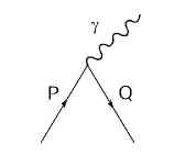
Figure 1: A forward particle $P$ interacts with a photon $\gamma$ and becomes a backward particle $Q$.

Therefore, one might think that there are no differences at all between forward and backward particles, since apparently the latter are always seen in the same way as the first ones. However, this is not so because whenever a backward particle is observed as a forward particle, some of its properties turns out to be switched in the process of observation. For instance, if a backward particle has a positive electric charge, say $+e$, then, due to the conservation of electric charge principle, we must actually observe a “switched” particle carrying the negative charge $-e$. Let us clarify this point through the following experiment.

Consider the phenomenon described in the Figure 1, which describes a forward particle $P$ with electric charge $+e$ who interact at some time with a photon $\gamma$ and, by virtue of this interaction, becomes a backward particle, $Q$. Note that the particle $Q$ actually is the same particle $P$, but now it is traveling back in time. Therefore, the actual electric charge of $Q$ is still $+e$. Nevertheless, when this process is physically observed, the observer should use (even unconsciously) the switching principle and the phenomenon is to be interpreted as follows: two particles of equal mass approach each to the other and, at some point, collide and annihilate themselves, which gives rise to a photon. Since the photon has no electric charge and the observed charge of the forward particle is $+e$ it follows that the observed charge of the backward particle has to be $-e$. The conclusion which follows from this is that the sign of the electric charge of a backward particle must be reversed in the process of observation.

Thus, a backward particle of mass $m$ and electric charge $+e$ should always be observed as a forward particle with the same mass and opposite electric charge. But these properties are precisely the same as expected to antiparticles. Therefore the switching principle enable us to interpret a backward particle as an antiparticle. The concept of antiparticles can be seen, hence, as a purely relativistic concept: it is not necessary to talk about quantum mechanics to introduce the concept of antiparticles.

Finally, let us remark that these arguments are also valid in the case of space-like particles, i.e., in the case of tachyons. In the section 8 we shall see that the energy of a tachyon is related to its momentum and mass through the relation $E^{2}=p^{2}c^{2}-m^{2}c^{4}$, an equation which describes now a single-sheet hyperboloid. From this we can see that tachyons must have an interesting property: they can change its status of a forward particle to the status of a backward one (and vice-versa) through a simple continuous motion. In other words, by accelerating a tachyon we can make it turn into an antitachyon and vice-versa (notice moreover that at some moment the tachyon must becomes a momentary particle, i.e., an particle with infinity velocity). This, of course, it is only possible to space-like particles.

4 Deduction of the extended Lorentz transformations (in two dimensions)

Let us show now how the Lorentz transformations can be generalized, or extended, to frames of reference moving with a velocity greater than that of light (as well as to frames of reference which travel back in time). In this section we shall discuss however the theory only in two dimensions. As commented before, we meet with several difficulties to formulating a theory of tachyons in four dimensions (these difficulties will be discussed in section 10). We shall give here two deductions for the Extended Lorentz Transformations (ELT), a algebraic deduction and a geometric one.

Algebraic Deduction: since in two dimensions the postulates presented on the previous sections are sufficient to proof that light propagates at the same speed $c$ for any inertial frame, we can take this result as our starting point.

So, consider a certain event whose coordinates are $\left(ct,x\right)$ with respect to an inertial frame $R$ and $\left(ct^{\prime},x^{\prime}\right)$ with respect to another inertial frame $R^{\prime}$ (which moves with the velocity $v$ with respect to $R$). Suppose further that the coordinate axes of these frames are always likely oriented and that the origin of $R$ and $R^{\prime}$ coincide when $t^{\prime}=t=0$.

Under these conditions, if a ray of light is emitted from the origin of these frames at $t=0$, then this ray will propagates with respect to $R$ according to the equation

$$x^{2}-c^{2}t^{2}=0,$$ (2)

and for $R^{\prime}$, by the principle of invariance of the speed of light, also by

$$x^{\prime 2}-c^{2}t^{\prime 2}=0.$$ (3)

(2) and (3) implies therefore,

$$x^{\prime 2}-c^{2}t^{\prime 2}=\lambda(v)\left(x^{2}-c^{2}t^{2}\right),$$ (4)

where $\lambda(v)$ does not depend on the coordinates and the time, but may depend on $v$.

In the other hand, since the frame $R$ moves with respect to $R^{\prime}$ with the velocity $-v$, follows also that

$$x^{2}-c^{2}t^{2}=\lambda(-v)\left(x^{\prime 2}-c^{2}t^{\prime 2}\right).$$ (5)

Therefore, from (4) and (5), we get $\lambda(v)\lambda(-v)=1$. Besides, the hypothesis of homogeneity and isotropy of space-time demands that $\lambda(v)$ does not depend on the velocity direction and then we are led to the condition

$$\lambda\left(v\right)^{2}=1\quad\Rightarrow\quad\lambda\left(v\right)=\pm 1.$$ (6)

Thus we have two cases to work on. Let us first analyze the first case, namely, $\lambda\left(v\right)=+1$. In this case the equation (4) becomes

$$x^{\prime 2}-c^{2}t^{\prime 2}=x^{2}-c^{2}t^{2},$$ (7)

whose solution, as it is known, is given by the usual Lorentz transformations,

$$ct^{\prime}=\frac{ct-xv/c}{\sqrt{1-v^{2}/c^{2}}},\quad x^{\prime}=\frac{x-vt}{\sqrt{1-v^{2}/c^{2}}}.$$ (8)

Note that these transformations contains the identity (for $v=0$) and they are discontinuous only at $v=\pm c$. Consequently, these transformations must be valid on the range $-v<c<v$ as well, but nothing can be said for $v$ out from this range.

In this way, we hope that in the other case, i.e., when $\lambda\left(v\right)=-1$, the respective transformations should be related to velocities greater than that of light. Now we will show that this is indeed what happens.

To $\lambda\left(v\right)=-1$, equation (4) becomes

$$x^{\prime 2}-c^{2}t^{\prime 2}=-\left(x^{2}-c^{2}t^{2}\right),$$ (9)

Through the formal substitutions $x\rightarrow\pm i\xi$ and $ct\rightarrow\pm ic\tau,$ we can rewrite (9) as

$$x^{\prime 2}-c^{2}t^{\prime 2}=\xi^{2}-c^{2}\tau^{2}.$$ (10)

Equation (10) has the same form as the equation (7) and therefore has the same solution:

$$ct^{\prime}=\frac{c\tau-\xi v/c}{\sqrt{1-v^{2}/c^{2}}},\quad x^{\prime}=\frac{\xi-v\tau}{\sqrt{1-v^{2}/c^{2}}}.$$ (11)

Expressing them back in terms of $x$ and $t$, we get

$$ct^{\prime}=\pm\frac{ct-xv/c}{\sqrt{v^{2}/c^{2}-1}},\quad x^{\prime}=\pm\frac{x-vt}{\sqrt{v^{2}/c^{2}-1}},$$ (12)

and we have just to remove the signals ambiguity on the expressions above. The correct sign, however, depends on the relatively direction of the frames $R$ and $R^{\prime}$ in their “moviment” on the space-time, and can be seen in the Figure (2). In the case of a forward space-like transformation, it is easy to show that the correct sign is the negative one.

Note that these equations, as well as those of the previous case, are discontinuous only for $v=\pm c$. But now they are real only when $|v|>c$. The equations (12) represent thus the Lorentz transformations between two space-like reference frames, that is, the transformations associated to $|v|>c$, where the correct sign depends if the frame $R^{\prime}$ is a forward or backward reference frame with respect to $R$ and can be determined by the Figure 2.

Geometrical Deduction: from the geometrical point of view, the ELT can be regarded as a (hyperbolic) rotation defined on the curve

$$\left|c^{2}t^{2}-x^{2}\right|=\rho^{2}.$$ (13)

We can call such a transformation as an extended hyperbolic rotation. Note that (13) represents a set of two orthogonal and equilateral hyperbolæ.

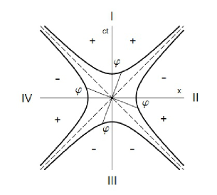
Figure 2: The Curve $\left|c^{2}t^{2}-x^{2}\right|=\rho^{2}.$

The asymptotes of this curve divide the plane onto four disjoint regions, namely, the regions I, II, III and IV, as show in the Figure 2.

To express such a rotation is convenient to introduce the extended hyperbolic functions, $\cosh\theta$ and $\sinh\theta$, defined by the following relations

$$ct=\rho\cosh\theta,\quad x=\rho\sinh\theta,$$ (14)

where $\theta$ is the usual circular parameter so that $0\leq\theta<2\pi$ and $\rho$ is given by (13). Note that in this geometric description the velocity $v$ is given by

$$v/c=\tanh\theta.$$ (15)

Expressions for $\cosh\theta$ and $\sinh\theta$ can be determined in several ways. For instance, we can use the usual hyperbolic functions $\cosh\varphi$ and $\sinh\varphi$ (where $\varphi$ is the usual hyperbolic parameter so that $-\infty<\varphi<+\infty$) to define them. Effectively, by introducing in each disjoint region of the space-time a hyperbolic parameter $\varphi$, which must be measured as shown in Figure 2, we can see that the functions $\cosh\varphi$ and $\sinh\varphi$ can be used to parametrize each one of the four branches of the curve (13). Once specified the region which $\theta$ belongs, $\rho$ and $\varphi$ determine in a unique way any point of the curve (13) and, therefore, they also determine the extended hyperbolic functions. With these conventions, we find out that

$$\begin{array}[]{c}\cosh\theta\equiv\begin{cases}+\cosh\varphi,&\theta\in\text{I}\\ -\sinh\varphi,&\theta\in\text{II}\\ -\cosh\varphi,&\theta\in\text{III}\\ +\sinh\varphi,&\theta\in\text{IV}\end{cases},\\ \\ \sinh\theta\equiv\begin{cases}+\sinh\varphi,&\theta\in\text{I}\\ +\cosh\varphi,&\theta\in\text{II}\\ -\sinh\varphi,&\theta\in\text{III}\\ -\cosh\varphi,&\theta\in\text{IV}\end{cases},\end{array}$$ (16)

where the parameters $\theta$ and $\varphi$ should be related by the formula

$$\tan\theta=\tanh\theta\equiv\begin{cases}+\tanh\varphi,&\theta\in\left(\text{I, III}\right)\\ -\coth\varphi,&\theta\in\left(\text{II, IV}\right)\end{cases}.$$ (17)

Expressions for the extended hyperbolic functions can also be found without making use of the usual hyperbolic functions. To do this, we parametrize (13) through the circular functions instead, putting $ct=r\cos\theta$ and $x=r\sin\theta$, with $r=\sqrt{c^{2}t^{2}+x^{2}}$. This allows us to write directly,

$$\cosh\theta=\frac{\cos\theta}{\sqrt{\left|\cos 2\theta\right|}},\quad\sinh\theta=\frac{\sin\theta}{\sqrt{\left|\cos 2\theta\right|}}.$$ (18)

or, in terms of the tangent,

$$\cosh\theta=\frac{\sigma(\theta)}{\sqrt{\left|1-\tan^{2}\theta\right|}},\quad\sinh\theta=\frac{\sigma(\theta)\tan\theta}{\sqrt{\left|1-\tan^{2}\theta\right|}},$$ (19)

where

$$\sigma(\theta)=\begin{cases}+1,&-\pi/2<\theta<\pi/2\\ -1,&\pi/2<\theta<3\pi/2\end{cases}.$$ (20)

The equivalence between (16) and (18) or (19) is found when one takes into account (17).

Once defined the extended hyperbolic functions it is easy

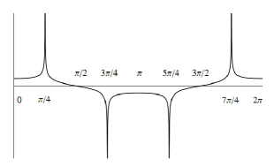
Figure 3: Graphic for the hyperbolic extended function $\cosh\theta$. The graphic of $\sinh\theta$ is similar to this, but with a phase difference of $\pi/2$ rad.

to obtain expressions describing an extended hyperbolic rotation. Let $\left(ct,x\right)=\left(\rho\cosh\theta_{1},\rho\sinh\theta_{1}\right)$ be the coordinates of a point on the plane with respect to a inertial coordinate system $R$, which it is assumed to belongs to the sector I of space-time. If we take a passive hyperbolic rotation (i.e., if we rotate the coordinate axes), say by an angle $\theta_{12}$, we shall obtain a new inertial coordinate system $R^{\prime}$ and the coordinates of that same point become $\left(ct^{\prime},x^{\prime}\right)=\left(\rho\cosh\theta_{2},\rho\sinh\theta_{2}\right)$ with respect to $R^{\prime}$. Since $\theta_{12}=\theta_{1}-\theta_{2}$, it follows that

$$ct^{\prime}=\rho\cosh\left(\theta_{1}-\theta_{12}\right),\quad x^{\prime}=\rho\sinh\left(\theta_{1}-\theta_{12}\right).$$ (21)

By replacing the expressions of $\cosh\left(\theta_{1}-\theta_{12}\right)$ and $\sinh\left(\theta_{1}-\theta_{12}\right)$ by any one of the above expressions and by simplifying the resulting expressions, taking also into account (17), we find out that $\left(ct^{\prime},x^{\prime}\right)$ is related to $\left(ct,x\right)$ through the equations

$$\begin{array}[]{c}ct^{\prime}=\delta\left(\theta_{12}\right)\left(ct\cosh\theta_{12}-x\sinh\theta_{12}\right),\\ \\ x^{\prime}=\delta\left(\theta_{12}\right)\left(x\cosh\theta_{12}-ct\sinh\theta_{12}\right),\end{array}$$ (22)

where

$$\delta\left(\theta\right)=\begin{cases}+1,&\tan^{2}\theta<1\\ -1,&\tan^{2}\theta>1\end{cases}.$$ (23)

Finally, using (19) and putting $\tan\theta_{12}=v/c$ , we obtain directly the required transformations, which are identical to those obtained before, namely,

$$ct^{\prime}=\varepsilon\left(\theta_{12}\right)\cfrac{ct-xv/c}{\sqrt{\left|1-v^{2}/c^{2}\right|}},\quad x^{\prime}=\varepsilon\left(\theta_{12}\right)\cfrac{x-vt}{\sqrt{\left|1-v^{2}/c^{2}\right|}},$$ (24)

where we put $\varepsilon\left(\theta_{12}\right)=\sigma\left(\theta_{12}\right)\delta\left(\theta_{12}\right)$. $\varepsilon\left(\theta_{12}\right)$ determines the correct sign which must appear in front of these transformations, as can be visualized in the Figure 2.

5 The composition law of velocities and inverse transformations

The transformations deduced in the previous sections do form a group. The ordinary Lorentz transformations is just a subgroup of it. Let us demonstrate now this group structure.

First, note that the identity is obtained with $v=0$. We shall show now that the composition of two ELT still results in another ELT. For this we introduce a third inertial frame $R^{\prime\prime}$, which moves with respect to $R^{\prime}$ with velocity $u=c\tanh\theta_{23}$. $R^{\prime}$ by its turn is assumed to moves with the velocity $u=c\tanh\theta_{12}$ with respect to $R$. We already know the transformation law between $R$ and $R^{\prime}$, and we can write it down:

$$\begin{array}[]{c}ct^{\prime}=\varepsilon\left(\theta_{12}\right)\cfrac{ct-x\tanh\theta_{12}}{\sqrt{\left|1-\tanh^{2}\theta_{12}\right|}},\\ \\ x^{\prime}=\varepsilon\left(\theta_{12}\right)\cfrac{x-ct\tanh\theta_{12}}{\sqrt{\left|1-\tanh^{2}\theta_{12}\right|}}.\end{array}$$ (25)

In its turn, the law of transformation from $R^{\prime}$ to $R^{\prime\prime}$ is given by an analogous expression:

$$\begin{array}[]{c}ct^{\prime\prime}=\varepsilon^{\prime}\left(\theta_{23}\right)\cfrac{ct^{\prime}-x^{\prime}\tanh\theta_{23}}{\sqrt{\left|1-\tanh^{2}\theta_{23}\right|}},\\ \\ x^{\prime\prime}=\varepsilon^{\prime}\left(\theta_{23}\right)\cfrac{x^{\prime}-ct^{\prime}\tanh\theta_{23}}{\sqrt{\left|1-\tanh^{2}\theta_{23}\right|}}.\end{array}$$ (26)

In these equations $\varepsilon^{\prime}\left(\theta_{23}\right)$ determines the signals corresponding to the transformation from $R^{\prime}$ to $R^{\prime\prime}$. These signals, however, do not need to equal necessarily the signals related to the transformation from $R$ to $R^{\prime}$. Indeed, while in the definition of $\varepsilon\left(\theta_{12}\right)$ the frame of reference $R$ was supposed to belong to the region I of space-time, the frame $R^{\prime}$ might belong to any region of space-time. Thus, $\varepsilon^{\prime}\left(\theta_{23}\right)$ should be regarded as a function to be yet determined.

Substitution of (25) into (26) gives us the law of transformation between $R$ and $R^{\prime\prime}$. After some simplifications, one can verify that the resulting expressions have the same form of the ELT, namely

$$\begin{array}[]{c}ct^{\prime\prime}=\varepsilon^{\prime\prime}\left(\theta_{13}\right)\cfrac{ct-x\tanh\left(\theta_{13}\right)}{\sqrt{\left|1-\tanh^{2}\left(\theta_{13}\right)\right|}}\\ \\ x^{\prime\prime}=\varepsilon^{\prime\prime}\left(\theta_{13}\right)\cfrac{x-ct\tanh\left(\theta_{13}\right)}{\sqrt{\left|1-\tanh^{2}\left(\theta_{13}\right)\right|}}.\end{array}$$ (27)

where

$$\varepsilon^{\prime\prime}\left(\theta_{13}\right)=\frac{\varepsilon\left(\theta_{12}\right)\varepsilon^{\prime}\left(\theta_{23}\right)}{\delta\left(\theta_{12},\theta_{23}\right)}$$ (28)

with

$$\delta\left(\theta_{12},\theta_{23}\right)=\begin{cases}+1,&\tanh\theta_{12}\tanh\theta_{23}<1\\ -1,&\tanh\theta_{12}\tanh\theta_{23}>1\end{cases},$$ (29)

and

$$\tanh\left(\theta_{13}\right)=\frac{\tanh\theta_{12}+\tanh\theta_{23}}{1+\tanh\theta_{12}\tanh\theta_{23}}=\tanh\left(\theta_{12}+\theta_{23}\right).$$ (30)

From (17) we can see that (30) consists of a generalization of the addition formula for the hyperbolic tangent, which reveals its geometric meaning. In terms of the velocity $v$, equation (30) can be rewritten as

$$w=\frac{u+v}{1+uv/c^{2}}.$$ (31)

Equation (31) expresses the composition law of velocities in this extended theory of relativity. It is exactly the same as predicted by the usual theory of relativity, but now it applies to any value of velocity.

Let we show also that the inverse transformation does exist. To do this, we impose onto (27) the conditions $ct^{\prime\prime}=ct$ and $x^{\prime\prime}=x$ and require that the resulting transformation be the identity. For this it is necessary to have $\theta_{23}=-\theta_{12}$ and $\varepsilon^{\prime\prime}\left(\theta_{13}\right)=1$, which enable us to evaluate $\varepsilon^{\prime}\left(\theta_{23}\right)$ from the resulting expression of $\varepsilon^{\prime\prime}\left(\theta_{13}\right)$. In fact, we find that

$$\varepsilon^{\prime}\left(\theta_{23}\right)=\delta\left(\theta_{12}\right)\big{/}\varepsilon\left(\theta_{12}\right)=\sigma\left(\theta_{12}\right),$$ (32)

since $\delta\left(\theta_{12},-\theta_{12}\right)=\delta\left(\theta_{12}\right)$, with $\delta\left(\theta_{12}\right)$ given (23).

Substituting this result into (26) we obtain the required expressions for the inverse transformations, which when expressed in terms of the velocity $v$ are given by

$$\begin{array}[]{c}ct=\varepsilon^{-1}\left(\theta_{12}\right)\cfrac{ct^{\prime}+x^{\prime}v/c}{\sqrt{\left|1-v^{2}/c^{2}\right|}},\\ \\ x=\varepsilon^{-1}\left(\theta_{12}\right)\cfrac{x^{\prime}+vt^{\prime}}{\sqrt{\left|1-v^{2}/c^{2}\right|}},\end{array}$$ (33)

and where we put $\varepsilon^{-1}\left(\theta_{12}\right)=\sigma\left(\theta_{12}\right)$.

Note that the signs appearing on the inverse transformation are different from that present on the direct transformations. This difference is a consequence of what was commented before, that in the transformation from $R$ to $R^{\prime}$ we had assumed the starting frame $R$ always belonging to the region I of space-time, while in the transformation from $R^{\prime}$ to $R$ it is the frame $R^{\prime}$ which is fixed on the region I. When $|v|<c$ this asymmetry has no effect at all, since in this case the signals are always the same in both expressions. But when $|v|>c$ however, we should alert that the inverse transformations can not be simply obtained by replacing $v$ by $-v$. It is still necessary multiply them by $-1$.

Finally, we mention that the associativity of ELT can be shown in a similar way, which completes the group structure of the ELT.

6 Conjugate Frames of Reference

We shall introduce now an important concept which can only be contemplated in an extended theory of relativity: the concept of conjugate frames of reference. The definition is the following: two frames of reference are said to be conjugate if their relative velocity is infinite. Thus, if $v$ is the velocity of the frame $R^{\prime}$ with respect to the frame $R$, the conjugate frame of reference associated to $R^{\prime}$ is another reference frame $R^{*}$, whose velocity is $w=c^{2}/v$ when measured by $R$. In fact, we obtain from (31),

$$\lim_{u\rightarrow\infty}\left(\frac{u+v}{1+uv/c^{2}}\right)=\frac{c^{2}}{v}.$$ (34)

Conjugate frames of reference are important because a space-like Lorentz transformation between two frames, say, from $R$ to $R^{\prime}$, can be obtained also by a usual Lorentz transformation between $R$ and $R^{*}$. For this, we simply have to replace $v\rightleftharpoons c^{2}/2$, $ct^{*}\rightleftharpoons x$ and $x^{*}\rightleftharpoons ct$. In fact, since $w=c^{2}/v$ is less than $c$ for $v>c$, it follows that the transformation from $R$ to $R^{*}$ is given by

$$ct^{*}=\frac{ct-xw/c}{\sqrt{1-w^{2}/c^{2}}},\quad x^{*}=\frac{x-wt}{\sqrt{1-w^{2}/c^{2}}}.$$ (35)

Making the replacements indicated above we can see in this way that we shall get the correct transformations between $R$ and $R^{\prime}$.

From a geometrical point of view the passage of a given frame of reference to its conjugate consists of a reflection of the coordinate axes relatively to the asymptotes of the curve (13), since this reflection precisely has the the effect of changing $ct$ by $x$ and vice-versa (and thus the effect of replacing $v$ by $c^{2}/v$). Therefore, we can see that an extended Lorentz transformation can be reduced to a usual Lorentz transformation by performing appropriate reflections relatively to asymptotes (in case of a space-like transformation) and around the origin (for a backward time-like transformation). This gives us a new way to derive the ELT.

It is interesting to notice also that, if a particle has velocity $u=c^{2}/v$ with respect to the frame $R$, then the velocity of this particle for the frame $R^{\prime}$ will be infinite. In other words this particle becomes a momentary particle to the frame $R^{\prime}$. More important than that, if the particle velocity $u$ is greater than $c^{2}/v$, and $v<c$, this particle becomes a backward particle to $R^{\prime}$ and it should be observed as an antiparticle by this reference frame. On the other hand, if $v>c$ the frame of reference $R^{\prime}$ should observe an antiparticle whenever $u<c^{2}/v$.

In an analogous way, since the frame $R^{\prime}$ moves with the velocity $-v$ with respect to $R$ , it follows also that a particle with velocity $u^{\prime}=c^{2}/v$ must have an infinite velocity with respect to $R$. So, in the case of $|v|<c$, the reference frame $R$ should observe an antiparticle if $u^{\prime}<c^{2}/v$ and, in the case of $|v|>c$, only if $u^{\prime}>-c^{2}/v$. These relationships might be, of course, more easily found by analyzing (30) or (31).

7 Rulers and clocks

Consider two identical clocks, one of them fixed in the frame $R$ and the other fixed to the frame $R^{\prime}$. Further, consider that these clocks are synchronized on $t=t^{\prime}=0$, where $R$ and $R^{\prime}$ are in the same position. We wish to compare the timing rate of these clocks, as measured by one of those frames. For example, suppose we want to compare the rhythm of these clocks when the time intervals are always measured by $R$. For this, suppose that the clock fixed on $R^{\prime}$ takes the time $\tau^{\prime}$ to complete a full period of oscillation. The time $T$ corresponding to this period of time, but now measured by $R$, can be found through the inverse transformations (33). Since this clock is at rest with respect to $R^{\prime}$, we should put $x^{\prime}=0$ on the first of the formulæ (33) and we shall get

$$T=\varepsilon^{-1}\left(\theta\right)\frac{\tau^{\prime}}{\sqrt{\left|1-v^{2}/c^{2}\right|}}.$$ (36)

Then, we can verify that a forward moving clock (with respect to $R$) becomes slower in measuring time than an identical clock at rest, when the speed of the clock is less than that of light (as it is well-known). But for a faster than light clock we get that it continues to be slower for $\left|v/c\right|<\sqrt{2}$ and it becomes faster when $\left|v/c\right|>\sqrt{2}$. It is interesting to note that for $\left|v/c\right|=\sqrt{2}$ both clocks go back to work at the same timing rate. Moreover, in the case of a backward moving clock, we can see from the switching principle that this clock should work in the counterclockwise, which is due to the fact that a backward-clock should mark the time from the future to the past.

Let us now verify what we got when the clocks are appreciated by the reference frame $R^{\prime}$. In this case we should use the direct transformations and thus we shall get

$$T^{\prime}=\varepsilon\left(\theta\right)\frac{\tau}{\sqrt{\left|1-v^{2}/c^{2}\right|}},$$ (37)

where $\tau$ is the time spent by the clock fixed at $R$ (which is moving with speed $-v$ with respect to $R^{\prime}$) for it to complete a full oscillation. Now, the signal appearing on (37) is determined according to the Figure 2 and the analysis becomes more or less complicated. Of course, we have no problems at all when $|v|<c$, then we shall analyze only the case where $|v|>c$. Suppose first that the reference frame $R^{\prime}$ is a forward frame with respect to $R$. In this case we find that $\varepsilon\left(\theta\right)=-1$ and the moving clock will work in the opposite direction as compared to the clock fixed at $R^{\prime}$. This means that the clock at $R$ is a backward-clock with respect to $R^{\prime}$. We can convince ourselves of this from what was commented in the previous section, where it is necessary to put there $u=0$ and $|v|>c$ (and therefore $u<c^{2}/v$).

This is an interesting situation indeed, because we have just seen that for the frame $R$, both clocks work clockwise (if the clocks are forward ones) or counterclockwise (if the clocks are backward ones) when $|v|>c$. In the other hand, for the frame $R^{\prime}$ if its own clock is working clockwise, then the moving clock should work counterclockwise and vice-versa. In the case where the reference frame $R^{\prime}$ is backward with respect to $R$ these asymmetries persists yet, but now is the frame $R$ which will see both clocks working differently, while for $R^{\prime}$ they will work accordingly. These asymmetries, of course, just express the fact that the extended Lorentz transformations, the direct and inverse one, are asymmetric by themselves in the case of $|v|>c$.

Let we consider now two identical rulers, one of them placed at rest in the frame $R$ and the other placed at rest with respect to $R^{\prime}$. We wish to compare the length of these rulers, when analyzed by one of these frames. If $l_{0}^{\prime}$ is the length of the ruler at $R^{\prime}$, when measured by this frame, the respective length $L$, as measured by $R$, is obtained by determining where the extreme points of the moving ruler is at a given instant $t$, say, $t=0$. Making use of the second equation of the direct transformations , we find that

$$L=\varepsilon\left(\theta\right)\cdot l_{0}^{\prime}\sqrt{\left|1-v^{2}/c^{2}\right|},$$ (38)

To $|v|<c$ we have the usual Lorentz contraction, but for $|v|>c$ we get that the moving ruler will be smaller than the ruler at rest when $\left|v/c\right|<\sqrt{2}$ . The rulers go back once again to have the same length when $\left|v/c\right|=\sqrt{2}$ and, finally, for $\left|v/c\right|>\sqrt{2}$ they should present a “Lorentz dilatation.” Moreover, regarding $R^{\prime}$ as a forward frame with respect to $R$, it follows that for the frame $R$ the moving ruler will be oriented contrarily with respect to the ruler at rest.

If, on the other hand, measurements are made by $R^{\prime}$, then we find that

$$L^{\prime}=\varepsilon^{-1}\left(\theta\right)\cdot l_{0}\sqrt{\left|1-v^{2}/c^{2}\right|},$$ (39)

and now for the reference frame $R$ the ruler at motion (which has the velocity $-v$) point out to the same direction as its ruler at rest. We find again the same asymmetry commented above for the clocks. These results can, of course, be more easily obtained – and fully understood – through Minkowski diagrams.

8 Dynamics

In this section we intend to answer some questions concerning the dynamics of tachyons. The expressions for the energy and momentum for a faster than light particle will be deducted and we shall show how these particles behave in the presence of a force field.

As a starting point we might assume that the principle of stationary action also applies to faster than light particles. This, of course, follows directly from the assumption of homogeneity and isotropy of space-time, since we know that this principle is true for slower than light for particles.

As one knows, the principle of stationary action states that there exist a quantity $S$, called action, which assumes an extreme value (maximum or minimum) for any possible movement of a mechanical system (in our case, a particle). On the other hand, in the absence of forces, the motion of a particle corresponds to a space-time geodesic, which reduces to a straight line by neglecting gravity. This means that in case of a free particle the differential of action $dS$ should be proportional to the line element $ds$ of the particle and we can write in this way

$$dS=\alpha ds,\quad ds=\sqrt{\left|c^{2}dt^{2}-dx^{2}-dy^{2}-dz^{2}\right|}.$$ (40)

We must emphasize, however, that the constant of proportionality $\alpha$ can take different values at different regions of space-time, since these regions are completely disconnected regions. Therefore, it is convenient to consider each case separately.

In the case of a forward and time-like particle, (40) takes the form

$$dS=\mathcal{L}\left(u\right)dt,\quad\mathcal{L}\left(u\right)=\alpha c\sqrt{1-u^{2}/c^{2}},$$ (41)

where we had introduced the LaGrange function, $\mathcal{L}\left(u\right)$, to express the action in terms of particle velocity.

As it is known, the expressions for the energy and momentum are obtained by the formulas

$$p\left(u\right)=\frac{\partial\mathcal{L}\left(u\right)}{\partial u},\quad E\left(u\right)=u\left[\frac{\partial\mathcal{L}\left(u\right)}{\partial u}\right]-\mathcal{L}\left(u\right).$$ (42)

Applying (42) onto (41) we obtain, thus

$$p\left(u\right)=-\frac{\alpha u/c}{\sqrt{1-u^{2}/c^{2}}},\quad E\left(u\right)=-\frac{\alpha c}{\sqrt{1-u^{2}/c^{2}}}.$$ (43)

To find $\alpha$ we may use the fact that for low speeds these expressions should reduce to that obtained by Newtonian mechanics. Thus, for instance, if we expand the expression for the momentum in a power series of $u/c$ and we keep only the first term, we should get $p\approx-\alpha u/c$, while Newtonian mechanics provides $p=mu$. Thus we get $\alpha=-mc$ and then

$$p\left(u\right)=\frac{mu}{\sqrt{1-u^{2}/c^{2}}},\quad E\left(u\right)=\frac{mc^{2}}{\sqrt{1-u^{2}/c^{2}}},$$ (44)

which are the same expressions of the usual theory of relativity.

In the case of a forward space-like particle (i.e. in the case of a forward tachyon), the LaGrange function takes the form

$$\mathcal{L}\left(u\right)=\alpha c\sqrt{u^{2}/c^{2}-1}.$$ (45)

and we get by (42), the following expressions for momentum and energy,

$$p\left(u\right)=\frac{\alpha u/c}{\sqrt{u^{2}/c^{2}-1}},\quad E\left(u\right)=\frac{\alpha c}{\sqrt{u^{2}/c^{2}-1}}.$$ (46)

The constant $\alpha$, however, no longer can be determined by comparing these expressions with those obtained in Newtonian mechanics, since the velocity of the particle is always greater than the speed of light in this case. But we can stead evaluate the limit of these expressions as $u\rightarrow\infty$, which give us

$$\lim_{u\rightarrow\infty}p\left(u\right)=\alpha,\quad\lim_{u\rightarrow\infty}E\left(u\right)=0,$$ (47)

by where we can see that $\alpha$ equals the momentum of a momentary particle, that is, the momentum of a infinitely fast particle.

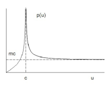
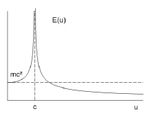
Figure 4: Graphics for the momentum and energy of a forward particle with speed $0\leq u<\infty$.

Since the mass of a particle must be a universal invariant, it follows that we can also define a metric in the space of energy and momenta. Making an analogy with $(\ref{eq:metrica})$, we can define this dynamic metric as

$$c^{2}dm=\sqrt{\left|dE^{2}-c^{2}dp_{x}^{2}-c^{2}dp_{y}^{2}-c^{2}dp_{z}^{2}\right|}.$$ (48)

Thus, it follows that the mass, the energy and the momentum must always be related by the formula $mc^{2}=\sqrt{\left|E^{2}-c^{2}p^{2}\right|}$ . If we put $E=0$ in this last equation, we get $p=mc$ (we had assumed that $p$ is positive for $u$ positive). We conclude in this way that the momentum and energy of a tachyon should be given by the expressions

$$p\left(u\right)=\frac{mu}{\sqrt{u^{2}/c^{2}-1}},\quad E\left(u\right)=\frac{mc^{2}}{\sqrt{u^{2}/c^{2}-1}}.$$ (49)

This result can also be obtained through the use of conjugate frames, introduced in section 6. Suppose a particle with velocity $u>c$ with respect to a reference frame $R$. Then, for the conjugate reference frame $R^{*}$ this particle will have energy $E^{*}=cp$ and momentum $p^{*}=E/c$, while its velocity becomes $w=c^{2}/u$, which is less than $c$. But the expressions for momentum and energy of a bradyon (i.e., a time-like particle) are given by (42) and we get, therefore

$$p^{*}=\frac{mw}{\sqrt{1-w^{2}/c^{2}}},\quad E^{*}=\frac{mc^{2}}{\sqrt{1-w^{2}/c^{2}}}.$$ (50)

We can verify in this way that the replacements of $E^{*}$, $p^{*}$ and $w$ into the above formulæ result exactly in the expression (49).

In the case of backward particles, the LaGrange function changes sign, since $dt$ is negative and $\mathcal{L}=dS/dt$. Therefore, backward particles must have a negative energy, a result which we had already indicated in section 3.

Finally, let us show how a space-like particle should behave when subjected to a force field. The expression for the force acting on the particle remains, of course, being given by Newton’s Law $\dot{p}=F$, but now $p$ is given by (49). Calculating the derivative, we obtain

$$F=-\frac{ma}{\left(u^{2}/c^{2}-1\right)^{3/2}},$$ (51)

where the $a=du/dt$ denotes the acceleration of the particle. Note that the force and the acceleration point out to opposite directions. Consequently, two space-like particles that attract (repel) must go far (go near) one from the other. The concepts of attraction/approximation and repulsion/expulsion, therefore, are no longer equivalent concepts when we deal with tachyons. In fact, if we try to approach (move away) from a tachyon, its relative speed decrease (increase), an effect that is contrary to our common sense but that can be demonstrated by a simple analysis of (31).

9 Causality and the Tolman Paradox

One of the arguments usually employed to show that faster than light particles can not exist is that their existence would imply a violation of the principle of causality. Indeed, suppose a tachyon is emitted by a body $A$ at time $t_{A}$ and it is absorbed by another body $B$ at time $t_{B}$, where $t_{B}>t_{A}$. Since these two events (emission of a tachyon by $A$ and its absorption by $B$) are separated by a space-like distance we know from the theory of relativity that it is possible to find a determined frame of reference (whose speed is less than that of light) where the chronological order of events is reversed. Thus, if we assume the event $A$ as the cause of the event $B$, we shall conclude then, for this moving frame of reference, that the effect precedes its cause.

Therefore, if we admit the concepts of cause and effect as absolute concepts and that the cause always precedes the effect, we would then effectively be led to the conclusion that faster than light particles can not exist. However, there is nothing from the mathematical point of view that supports this hypothesis. On the contrary, if we assume a complete isotropy and homogeneity of space-time, we have no choice but to consider the concepts of cause and effect as relative concepts.

We already had seen, of course, other quantities which were regarded as absolute in the usual theory of relativity and now they had to be seen as relative quantities. An example of this is the concept of emission and absorption. Indeed, since by the switching principle we did not observe backward-particles but only forward-antiparticles, the processes of emission (absorption) of backward-particles should always be observed as an absorption (emission) of forward-antiparticles. We can, of course, find out if a particle was actually emitted (absorbed) by analyzing the process in the frame where the source (emitter) is at rest, in this case we shall speak of an intrinsic or proper emission (absorption).

Nevertheless, the relative nature of causality does not lead to any contradiction into the theory. In nature, a phenomenon never describes an isolated event but only a continuous succession of events, which we shall call a physical process. Geometrically, a physical process describes a continuous curve in space-time and therefore has an absolute character: the order in time in which events occur may differ from a reference frame to another but the curve itself, which corresponds to the phenomenon in question, should be the same for any of them. This is enough for instance to show that we can not go back in time and kill our grandfather. In fact, the mere fact of our existence means that there exists a curve in space-time connecting our grandfather to us, and since this curve has an absolute character, it can not be disconnected to any observer, even backing in time.

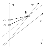
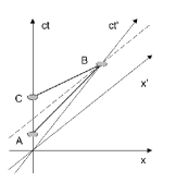
Figure 5: Experiment devised by Tolman.

As an example of a paradox which involves the concept of causality, let us examine the interesting paradox proposed and discussed by Tolman [15] in 1917 (although it had been pointed out ten years earlier by Einstein [16]). Further details can be checked in [17, 18, 19].

The paradox consists in showing that if faster than light particles does exist, then it would be possible to send information to the past. To show this, consider the references $R$ and $R^{\prime}$ (with $R^{\prime}$ moving with speed $v<c$ with respect to $R$) are equipped with some special phone devices, whose communication is done through the transmission of tachyons. Imagine, then, that an observer $R$ sends a message (event $A$), for instance in the form of a question, to $R^{\prime}$ and that after he had received (event B), $R^{\prime}$ sends back his answer to $R$, which is then received by $R$ (event $C$). It turns out that, as seen in Figure 5a, the observer $R^{\prime}$ can calibrate its device in such a way that the message sent by him arrives at $R$ even before $R$ had sent its question. Thus, since $R$ got the answer before he had make the ask, he might decides to not do the question, in which case we shall meet to a very paradoxical situation.

The failure on this argument is that it mixes the descriptions of the reference frames when the terms “emition” and “absorption” are employed. In fact, we shall show now (following [4]) that if the frame of reference $R^{\prime}$ intrinsically receives the question submitted by $R$, as well as he intrinsically sends its answer, then the frame of reference $R$ should always receive the reply after he had make the ask.

For this, suppose that the question of $R$ is sent with velocity $u_{1}$ and the answer comes back with the velocity $u_{2}$, where $u_{1}$ and $u{}_{2}$ are greater than the speed of light and they are always measured by $R$. Notice then that for the answer of $R^{\prime}$ arrives before the question sent by $R$ it is necessary to have $\left|u_{1}\right|>\left|u_{2}\right|$ because for $R$ the event $C$ occurs before $A$ and both arrive on $B$ at the same time. Nevertheless, for the frame of reference $R^{\prime}$ to receive intrinsically the question sent by $R$ it is necessary to have $\left|u_{1}\right|<c^{2}/v$, since in the other case, as we have seen in section 6, this message would be a backward-message to $R^{\prime}$ and hence $R^{\prime}$ would simply see the emission of the message by transmission of antitachyons as predicted by the switching principle. Similarly, for $R^{\prime}$ intrinsically to send its answer, we must have $\left|u_{2}\right|>c^{2}/v$, since the answer is sent in the negative direction of the axis $X$ of $R$. Thus, we had show that $\left|u_{2}\right|>\left|u_{1}\right|$, a contradiction.

Therefore, if the reference $R^{\prime}$ effectively receives the question sent from $R$ and effectively sends her answer, the process must be described by the Figure 5b, not by the Figure 5a. In this case, the answer always comes after the question sent by $R$.

Of course, the Figure 5a also represents a valid physical process, but not one as described by the Tolman paradox. Each frame of reference should have its own view of what is actually happening in it. For instance, for $R$ the experiment described by Figure 5a corresponds to the case where there is, first, the emission of the message $C$ (through an antitachyon jet) and soon after, there is the emission of the message $A$ (via a tachyon jet); finally, both messages come together at $B$. But for $R^{\prime}$ all happens as he had sent the message $C$ to $R$ by an antitachyon jet and, at the same time, sent the message $A$ by means of a tachyons jet; then after some time the observer $R$ would receive the message $C$ and then the message $A$. Note that the chronological order of the events depends on the frame considered, but the process itself (which connects the events $A$, $B$ and $C$) is unique.

10 Difficulties for formulating the theory of tachyons in four dimensions

In the section 4 we show that in two dimensions the Lorentz transformations can be extended in order to relate any imaginable pair of inertial frames. When, however, we try to do the same in four dimensions we meet with serious difficulties, which we shall briefly discuss now.

Let us remind the reader that by extending the Lorentz transformations in two dimensions, we had made use of an important principle, which states that the speed of light is the same in any inertial frame. We saw, moreover, that this principle can be deduced from the postulates presented in section 2, and hence this principle can be seen as a theorem of the relativity theory. When, however, we pass to a universe in four dimensions, is no longer possible to proof the general validity of this theorem, in the same way as we did in two dimensions. Actually, in four dimensions we can not even say that light travels in spherical surfaces with speed $c$ in all inertial frame of reference (it is only in the case of $v<c$ we can mathematically proof this assertion, from the postulates of relativity).

To show more clearly why we meet with these difficulties, let us consider for example a source of light fixed on the origin of the frame $R$ and suppose that with respect to this frame light propagates in spherical surfaces with velocity $c$. In four-dimensional space-time the asymptotes are replaced by a cone – the light cone. The geometric region of space-time associated to a beam of light (emitted by the source fixed at the origin of the reference frame $R$) always belongs to this light cone.

The usual theory of relativity also shows that for any other time-like frame of reference, the propagation of light is still represented by the same light cone. But how should the light behave itself with respect to a space-like frame, say, $R^{\prime}$? In this case, the time axis of this frame always point out to the outside region of the light cone of $R$, so that is not evident that the light emitted by the source fixed at $R$ should also propagates in spherical surfaces with speed $c$ with respect to $R^{\prime}$. Beside this, we might ask what happens when a light source is fixed on $R^{\prime}$. Does the light emitted by this source propagates in spherical surfaces with speed $c$ with respect to $R^{\prime}$? And what is to be said with respect to the frame $R$, where the source has velocity $v>c$, does the light propagates spherical waves with speed $c$?

As one can see, there are several issues that can not be answered immediately, not without having additional information. Indeed, the behavior of light depends on its intrinsic properties, and these properties are determined by a extended theory of electromagnetism which is a priori unknown. Let us examine these possibilities a little more.

We can suppose for instance that the source of light fixed at $R^{\prime}$ (which we shall suppose to have a velocity greater than $c$, with respect to $R$) also emits spherical waves with speed $c$, when measured by $R^{\prime}$. So, there must exist now another light cone corresponding to space-like frames of reference, a cone which must contour the axis of time of $R^{\prime}$. Since the axis of time of $R$ always should be outside from this new light cone, it follows that for $R$ the light emitted by the moving source will not propagates into spherical surfaces of speed $c$, but rather it will take a form of a two-sheet hyperboloid surface. In this case the speed of light would depend of the direction and space-time could no longer be considered isotropic anymore.

If, in other hand, we regard that the light emitted by the source fixed on $R^{\prime}$ also propagates in spherical surfaces with respect to the reference frame $R$, that is, that there are a unique light cone in the universe by where the light always “travels”, no matter what is the speed of the source, then we can see that, although for $R$ the light propagates in spheres of speed $c$, now the same is not true for $R^{\prime}$, which should observes the light to propagating in a two-sheet hyperboloid.

For light spread in spherical surfaces and with velocity $c$ to both reference frames is necessary that the transverse coordinates, $y^{\prime}$ and $z^{\prime}$ of the frame $R^{\prime}$ be imaginary quantities (assuming $y$ and $z$ real). Indeed, just in this case we can map a “time-like light cone” to a “space-like light cone.” Effectively, this can be shown by deducing the ELT in four dimensions, assuming from the start the validity of the principle of invariance of the speed of light to any inertial frame. We have in this case,

$$x^{\prime 2}+y^{\prime 2}+z^{\prime 2}-c^{2}t^{\prime 2}=\lambda\left(v\right)\left(x^{2}+y^{2}+z^{2}-c^{2}t^{2}\right),$$ (52)

in place of (4). As it is known, the solution of this equation for $\lambda\left(v\right)=+1$ consists of the usual Lorentz transformations, while for $\lambda\left(v\right)=-1$ we shall get

$$\begin{array}[]{c}ct^{\prime}=\pm\cfrac{ct-xv/c}{\sqrt{v^{2}/c^{2}-1}},\quad x^{\prime}=\pm\cfrac{x-vt}{\sqrt{v^{2}/c^{2}-1}},\\ \\ y^{\prime}=\pm iy,\quad z^{\prime}=\pm iz,\end{array}$$ (53)

and the transverse coordinates $y^{\prime}$ and $z^{\prime}$ become imaginary. The introduction of imaginary coordinates is, however, deprived of physical sense.

If, by its turn, we deny the validity of the principle of invariance of the speed of light, then we obtain the transformations

$$\begin{array}[]{c}ct^{\prime}=\pm\cfrac{ct-xv/c}{\sqrt{v^{2}/c^{2}-1}},\quad x^{\prime}=\pm\cfrac{x-vt}{\sqrt{v^{2}/c^{2}-1}},\\ \\ y^{\prime}=\pm y,\quad z^{\prime}=\pm z.\end{array}$$ (54)

where now all coordinates are real. The problem here is that we lie in the cases discussed above, where the space-time can not be considered isotropic.

Note that in each one of the possibilities discussed above, the transverse components of the physical quantities become different. Thus, for example, the formulation of the electrodynamics of tachyons will assume different forms in each one of these formulations. Only the experiment can decides which one or another is the correct, (assuming that someone of them are correct).

In short, the arguments presented above show us that in a four-dimensional universe we can not extend the Lorentz transformations in order to satisfy all the postulates presented in section 2, unless it is introduced imaginary quantities, which has no physical interpretation. We shall see in the next section that, if we not impose the validity of the postulate $1$, i.e. that the universe is four-dimensional, then it becomes possible to build up a theory of tachyons which satisfy the other postulates fully.

11 An possible theory in six dimensions

We might wonder why we find difficulties on extending the Lorentz transformations in a four-dimensional universe if in a two-dimensional universe this generalization is straightforward. We can figure out what is happening by reflecting a little about. The reason by which this occurs lies in the fact that in four dimensions the number of space-like dimensions is different from the number of time-like dimensions (3 space-like dimensions against 1 time-like dimension). Since experience shows us that the universe has three space-like dimensions (at least), it follows that we must consider a six-dimensional universe (at least) – 3 space-like dimensions against other 3 time-like dimensions.

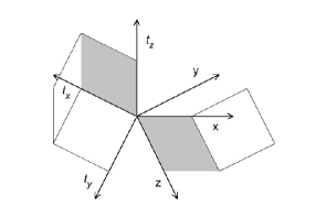
Figure 6: An illustration for the six-dimensional universe – “orthogonal universes.”

But what is to be understood by a universe with three time-like dimensions? The interpretation we propose here is the following: although this universe has three time-like dimensions, the physical time, that is, the time which is actually measured by an observer, is always a one-dimensional quantity. Indeed, this physical time must match with the proper-time of the observer, that is, it should be determined by the world line length of the observer concerned.

Thus, for consistence, we should consider also that the other two time-like dimensions which are orthogonal to the observer’s world line, should be always inaccessible to this observer. Therefore, although we regard the universe as six-dimensional in nature, the physical universe happens to be just four-dimensional. In such a way, this six-dimensional universe can be interpreted as consisting of two orthogonal dimensional universes of three dimension each.

These interpretations enable us to define a six-dimensional metric for this universe by the expression

$$ds=\sqrt{\left|c^{2}dt_{x}^{2}+c^{2}dt_{y}^{2}+c^{2}dt_{z}^{2}-dx^{2}-dy^{2}-dz^{2}\right|},$$ (55)

and a physical metric by

$$d\sigma=\sqrt{\left|c^{2}dt_{x}^{2}-dx^{2}-dy^{2}-dz^{2}\right|},$$ (56)

where we suppose $t_{x}$ as the physical time measured by the observer (by a convenient choice of the coordinate system, this can always be done, of course).

Let us then show now how one can get the ELT in complete agreement with the relativity postulates presented in section 2. For this, let a particular event has coordinates $\left(ct_{x},ct_{y},ct_{z},x,y,z\right)$ with respect to $R$, but suppose furthermore that only the coordinates $\left(ct_{x},x,y,z\right)$ are accessible to this reference frame. Similarly, for the reference frame $R^{\prime}$ let $\left(ct_{x}^{\prime},ct_{y}^{\prime},ct_{z}^{\prime},x^{\prime},y^{\prime},z^{\prime}\right)$ be the coordinates of that same event, and suppose now that only the coordinates $\left(ct_{x}^{\prime},x^{\prime},y^{\prime},z^{\prime}\right)$ are accessible to $R^{\prime}$.

Let we analyze first the case where $v<c$. It is evident in this case that the accessible dimensions to $R$ and $R^{\prime}$ should coincide themselves (in fact, this is true for $v=0$ and therefore the result must continuity requirement). Thus, we obtain directly that the transformations should be just the usual Lorentz transformations, plus the relations

$$ct_{y}^{\prime}=ct_{y},\quad ct_{z}^{\prime}=ct_{z},\quad y^{\prime}=y,\quad z^{\prime}=z.$$ (57)

Consider now the more interesting case where $v>c$. Here, on the contrary, there must be a reversal of the accessible dimensions of $R$ when they are observed by $R^{\prime}$. Indeed, one might say, for instance, that the frames of reference $R$ and $R^{\prime}$ are now in differents “orthogonal universes.” Thus, the coordinates $ct_{y}$ and $ct_{z}$ should become accessible to $R^{\prime}$, while the coordinates $y$ and $z$ should become inaccessible to him. Note also that the necessary condition for the light propagates in spherical surfaces with speed $c$ in both frames of reference is only that one has $d\sigma^{\prime}=d\sigma=0$ for rays of light. Nevertheless, we can consider a stronger hypothesis, namely, that in the six-dimensional universe the light propagates accordingly the equation $ds^{\prime}=ds=0$. In this case it is easy to verify that the previous condition is satisfied as well if we write

$$ct_{y}^{\prime}=\pm y,\quad ct_{z}^{\prime}=\pm z,\quad y^{\prime}=\pm ct_{y},\quad z^{\prime}=\pm ct_{z},$$ (58)

which must to be added to the expressions

$$ct_{x}^{\prime}=\pm\frac{ct_{x}-xv/c}{\sqrt{v^{2}/c^{2}-1}},\quad x^{\prime}=\pm\frac{x-vt_{x}}{\sqrt{v^{2}/c^{2}-1}},$$ (59)

already deduced in the section 4. These equations constitute the ELT related to this six-dimensional universe. Notice, in special, that all coordinates are real.

Let us finally interpret the results. In the first place, is easy to see that in both frames of reference light propagates with speed $c$. This can be done by direct substitution of (58) and (59) into (56). In addition, notice that in this formulation, tachyons might be observed in the reference $R$ with a shape very different from what they present to $R^{\prime}$ because to the reference $R$ the transverse coordinates are given by $y=\pm ct_{y}^{\prime}$ and $z=\pm ct_{z}^{\prime}$, which are not accessible to $R^{\prime}$.

Further, it is interesting to notice that if a source of light is fixed to the frame $R^{\prime}$, then the frame $R$ should see the light propagating in spherical surfaces with speed $c$, as we had shown. But since the source has in this case a velocity greater than $c$, we must have the formation of a Mach cone in fact, since the source is always ahead from the waves which it emits. One can show that the superposition of waves emitted by a superluminal source results at two front waves whose shapes have the form of a two-sheet hyperboloid surface. The group velocity of these waves depends on the direction, being always larger than $c$ (except in the direction $X$ whose velocity equals $c$). This, however, is due purely to an interference phenomenon, unlike the cases of the previous formulations, which this phenomenon was due to a anisotropy of space-time itself.

This kind of waves are often called “$X$ waves”, they are superluminal solutions of the Maxwell’s equations [21, 22] – these waves have indeed been observed and even produced in the laboratory [3, 21, 22, 23]. This is an important experimental verification of the existence of superluminal phenomena in nature.

References

- [1] T. Adam et Al. (The OPERA Collaboration), Measurement of the neutrino velocity with the OPERA detector in the CNGS beam, arXiv:1109.4897v1 [hep-ex], p. 1-24, (2011).
- [2] R.S. Vieira, Para Além da Velocidade da Luz – Uma Breve Introdução à Teoria dos Tachyons, Palestra apresentada na 7ª Semana da Física da Universidade Federal de São Carlos, São Carlos, (2011).
- [3] E. Recami, Superluminal motions? A bird-eye view of the experimental situation, Found. Phys., 31, p. 1119–1135, (2001).
- [4] E. Recami, Classical Tachyons and Possible Applications, Riv. Nuovo Cim. vol. 9, s. 3, n. 6, p. 1-178, (1986).
- [5] H. Poincaré, Sur la dynamique de l’électron, Circ. Mat. Palermo, 21, p. 129–176 (1906).
- [6] H. Minkowski, Raum und Zeit, Phys. Z. 10, p. 104-111, (1909).
- [7] P.A.M. Dirac, A Teory of electrons and protons, Proc. R. Soc. London, A 126, p. 360-365 (1930).
- [8] E.C.G. Stückelberg, Remarque a Propos de la Création de Paires de Particules en Théorie de Relativité, Helv. Phys. Acta, 14, p. 588-594, (1941).
- [9] E.C.G. Stückelberg, La mécanique du point matériel en théorie de relativité et en théorie des quanta, Helv. Phys. Acta, 15, p. 23-37, (1942).
- [10] R.P. Feynman, Space-Time Approach to Quantum Electrodynamics, Phys. Rev. 76, p. 769-789, (1949).
- [11] R.P. Feynman, The reason for antiparticles, in Elementary Particles and the Laws of Physics, The 1986 Dirac Memorial Lectures by R.P. Feynman and S. Weinberg, (Cambridge University Press, Cambridge, 1987).
- [12] O.M.P. Bilaniuk, V.K. Deshpande e E.C.G. Sudarshan, “Meta” Relativity, Am. Journ. Phys., 30, p. 718-723, (1962).
- [13] F. Catoni et Al., The Geometry of Minkowski Space-Time, (Springer Briefs in Physics, 2011).
- [14] J. Vaz Jr., A Álgebra Geométrica do Espaço-tempo e a Teoria da Relatividade, Rev. Bras. Ens. Física, 22, p. 5-31, (2000).
- [15] R.C. Tolman, The Theory of Relativity of Motion, (Berkeley, 1917).
- [16] A. Einstein, Über die vom Relativitätsprinzip geforderte Trägheit der Energie, Ann. d. Phys. 23, p. 371-384, (1907).
- [17] D. Bohm, The Special Theory of Relativity, (New York, 1965).
- [18] E. Recami, The Tolman ‘antitelephone’ paradox: It’s solution by tachyon mechanics, Lett. Nuovo Cim. 44, p. 587-593, (1985).
- [19] E. Recami, Tachyon kinematics and causality: A systematic, thorough analysis of the tachyon causal paradoxes, Found. Phys., 17, p. 239-296 (1987).
- [20] R.L. Dawe, K.C. Hines, The Physics of Tachyons I. Tachyon Kinematics, Aust. J. Phys. 45, p. 591-620, (1992).
- [21] E.C. de Oliveira, W.A. Rodrigues Jr., Soluções Superluminais de Enegia finita das Equações de Maxwell, Tend. Mat. Apl. Comput., 3, p. 165-171, (2002).
- [22] E. Recami, M.Z. Rached, Localized Waves: A not-so-short Review, Advances in Imaging & Electron Physics, 156, p. 235-355, (2009).
- [23] E. Recami, M. Fracastoro-Decker, W.A. Rodrigues Jr., Táquions, Revista Ciência Hoje, 5, n. 26, p. 48-59 (1986); E. Recami, M.Z. Rached, Mais velozes que a luz? Revista Ciência Hoje, 29, n. 170, p. 20-25 (2001).