A conjugate gradient algorithm
for the astrometric core solution of Gaia

Abstract

Context. The ESA space astrometry mission Gaia, planned to be launched in 2013, has been designed to make angular measurements on a global scale with micro-arcsecond accuracy. A key component of the data processing for Gaia is the astrometric core solution, which must implement an efficient and accurate numerical algorithm to solve the resulting, extremely large least-squares problem. The Astrometric Global Iterative Solution (AGIS) is a framework that allows to implement a range of different iterative solution schemes suitable for a scanning astrometric satellite.

Aims. Our aim is to find a computationally efficient and numerically accurate iteration scheme for the astrometric solution, compatible with the AGIS framework, and a convergence criterion for deciding when to stop the iterations.

Methods. We study an adaptation of the classical conjugate gradient (CG) algorithm, and compare it to the so-called simple iteration (SI) scheme that was previously known to converge for this problem, although very slowly. The different schemes are implemented within a software test bed for AGIS known as AGISLab. This allows to define, simulate and study scaled astrometric core solutions with a much smaller number of unknowns than in AGIS, and therefore to perform a large number of numerical experiments in a reasonable time. After successful testing in AGISLab, the CG scheme has been implemented also in AGIS.

Results. The two algorithms CG and SI eventually converge to identical solutions, to within the numerical noise (of the order of 0.00001 micro-arcsec). These solutions are moreover independent of the starting values (initial star catalogue), and we conclude that they are equivalent to a rigorous least-squares estimation of the astrometric parameters. The CG scheme converges up to a factor four faster than SI in the tested cases, and in particular spatially correlated truncation errors are much more efficiently damped out with the CG scheme. While it appears to be difficult to define a strict and robust convergence criterion, we have found that the sizes of the updates, and possibly the correlations between the updates in successive iterations, provide useful clues.

1 Introduction

The European Space Agency’s Gaia mission (Perryman et al. 2001; Lindegren et al. 2008; Lindegren 2010) is designed to measure the astrometric parameters (positions, proper motions and parallaxes) of around one billion objects, mainly stars belonging to the Milky Way Galaxy and the local group. The scientific processing of the Gaia observations is a complex task that requires the collaboration of many scientists and engineers with a broad range of expertise from software development to CCDs. A consortium of European research centres and universities, the Gaia Data Processing and Analysis Consortium (DPAC), has been set up in 2005 with the goal to design, implement and operate this process (Mignard et al. 2008). In this paper we focus on a central component of the scheme, namely the astrometric core solution, which solves the corresponding least-squares problem within a software framework known as the Astrometric Global Iterative Solution, or AGIS (Lammers et al. 2009; Lindegren et al. 2011; O’Mullane et al. 2011).

In a single solution, the AGIS software will simultaneously calibrate the instrument, determine the three-dimensional orientation (attitude) of the instrument as a function of time, produce the catalogue of astrometric parameters of the stars, and link it to an adopted celestial reference frame. This computation is based on the results of a preceding treatment of the raw satellite data, basically giving the measured transit times of the stars in the instrument focal plane (Lindegren 2010). The astrometric core solution can be considered as a least-squares problem with negligible non-linearities except for the outlier treatment. Indeed, it should only take into account so-called primary sources, that is stars and other point-like objects (such as quasars) that can astrometrically be treated as single stars to the required accuracy. The selection of the primary sources is a key component of the astrometric solution, since the more that are used the better the instrument can be calibrated, the more accurate the attitude can be determined, and the better the final catalogue will be. This selection, and the identification of outliers among the individual observations, will be made recursively after reviewing the residuals of previous solutions (Lindegren et al. 2011). What remains is then, ideally, a ‘clean’ set of data referring to the observations of primary sources, from which the astrometric core solution will be computed by means of AGIS.

From current estimates, based on the known instrument capabilities and star counts from a Galaxy model, it is expected that at least 100 million primary sources will be used in AGIS. Nonetheless, the solution would be strengthened if even more primary sources could be used. Moreover, it should be remembered that AGIS will be run many times as part of a cyclic data reduction scheme, where the (provisional) output of AGIS is used to improve the raw data treatment (the Intermediate Data Update; see O’Mullane et al. 2009). Hence, it is important to ensure that AGIS can be run both very efficiently from a computational viewpoint, and that the end results are numerically accurate, i.e., very close to the true solution of the given least-squares problem.

Based on the generic principle of self-calibration, the attitude and calibration parameters are derived from the same set of observational data as the astrometric parameters. The resulting strong coupling between the different kinds of parameters makes a direct solution of the resulting equations extremely difficult, or even unfeasible by several orders of magnitude with current computing resources (Bombrun et al. 2010). On the other hand, this coupling is well suited for a block-wise organization of the equations, where, for example, all the equations for a given source are grouped together and solved, assuming that the relevant attitude and calibration parameters are already known. The problem then is of course that, in order to compute the astrometric parameters of the sources to a given accuracy, one needs to know first the attitude and calibration parameters to corresponding accuracies; these in turn can only be computed once the source parameters have been obtained to sufficient accuracy; and so on. This organization of the computations therefore naturally leads to an iterative solution process. Indeed, in AGIS the astrometric solution is broken down into (at least) three distinct blocks, corresponding to the source, attitude and calibration parameter updates, and the software is designed to optimize data throughput within this general processing framework (Lammers et al. 2009). Cyclically computing and applying the updates in these blocks corresponds to the so-called simple iteration (SI) scheme (Sect. 2.1), which is known to converge, although very slowly.

However, it is possible to implement many other iterative algorithms within this same processing framework, and some of them may exhibit better convergence properties than the SI scheme. For example, it is possible to speed up the convergence if the updates indicated by the simple iterations are extrapolated by a certain factor. More sophisticated algorithms could be derived from various iterative solution methods described in the literature.

The purpose of this paper is to describe one specific such algorithm, namely the conjugate gradient (CG) algorithm with a Gauss–Seidel preconditioner, and to show how it can be implemented within the AGIS processing framework. We want to make it plausible that it indeed provides a rigorous solution to the given least-squares problem. Also, we will study its convergence properties in comparison to the SI scheme and, if possible, derive a convergence criterion for stopping the iterations.

Our focus is on the high-level adaptation of the CG algorithm to the present problem, i.e., how the results from the different updating blocks in AGIS can be combined to provide the desired speed-up of the convergence. To test this, and to verify that the algorithm provides the correct results, we need to conduct many numerical experiments, including the simulation of input data with well-defined statistical properties, and iterate the solutions to the full precision allowed by the computer arithmetic. On the other hand, since it is not our purpose to validate the detailed source, instrument and attitude models employed by the updating blocks, we can accept a number of simplifications in the modelling of the data, such that the experiments can be completed in a reasonable time. The main simplifications used in the present study are as follows:

1. For conciseness we limit the present study to the source and attitude parameters, whose mutual disentanglement is by far the most critical for a successful astrometric solution (cf. Bombrun et al. 2010). For the final data reduction many calibration parameters must also be included, as well as global parameters (such as the PPN parameter $\gamma$; Hobbs et al. 2010), and possibly correction terms to the barycentric velocity of Gaia derived from stellar aberration (Butkevich & Klioner 2008). These extensions, within the CG scheme, have been implemented in AGIS but are not considered here.

2. We use a scaled-down version of AGIS, known as AGISLab (Sect. 4.1), which makes it possible to generate input data and perform solutions with a much smaller number of primary sources than would be required for the (full-scale) AGIS system. This reduces computing time by a large factor, while retaining the strong mutual entanglement of the source and attitude parameters, which is the main reason why the astrometric solution is so difficult to compute.

3. The rotation of the satellite is assumed to follow the so-called nominal scanning law, which is an analytical prescription for the pointing of the Gaia telescopes as a function of time. That is, we ignore the small ($<1$ arcmin) pointing errors that the real mission will have, as well as attitude irregularities, data gaps, etc. The advantage is that the attitude modelling becomes comparatively simple and can use a smaller set of attitude parameters, compatible with the scaled-down version of the solution.

4. The input data are ‘clean’ in the sense that there are no outliers, and the observation noise is unbiased with known standard deviation. This highly idealised condition is important in order to test that the solution itself does not introduce unwanted biases and other distortions of the results.

An iterative scheme should in each iteration compute a better approximation to the exact solution of the least-squares problem. In this paper we aim to demonstrate that the SI and CG schemes are converging in the sense that the errors, relative to an exact solution, vanish for a sufficient number of iterations. Since we work with simulated data, we have a reference point in the true values of the source parameters (positions, proper motions and parallaxes) used to generate the observations. We also aim to demonstrate that the CG method is an efficient scheme to solve the astrometric least-squares problem, i.e., that it leads, in a reasonable number of iterations, to an approximation that is sufficiently close to the exact solution. An important problem when using iterative solution methods is how to know when to stop, and we study some possible convergence criteria with the aim to reach the maximum possible numerical accuracy.

The paper provides both a detailed presentation of the SI and CG algorithms at work in AGIS and a study of their numerical behaviour through the use of the AGISLab software (Holl et al. 2010). The paper is organized as follows: Section 2 gives a brief overview of iterative methods to solve a linear least-squares problem. Section 3 describes in detail the algorithms considered here, viz., the SI and CG with different preconditioners. In Sect. 4 we analyze the convergence of these algorithms and some properties of the solution itself. Then, Sect. 5 presents the implementation status of the CG scheme in AGIS before the main findings of the paper are summarized in the concluding Sect. 6.

2 Iterative solution methods

This section presents the mathematical basis of the simple iteration and conjugate gradient algorithms to solve the linear least-squares problem. For a more detailed description of these and other iterative solution methods we refer to Björck (1996) and van der Vorst (2003). A history of the conjugate gradient method can be found in Golub & O’Leary (1989).

Let $\@vec{M}\@vec{x}=\@vec{h}$ be the overdetermined set of observation (design) equations, where $\@vec{x}$ is the vector of unknowns, $\@vec{M}$ the design matrix, and $\@vec{h}$ the right-hand side of the design equations. The unknowns are assumed to be (small) corrections to a fixed set of reference values for the source and attitude parameters. These reference values must be close enough to the exact solution that non-linearities in $\@vec{x}$ can be neglected; thus $\@vec{x}=\@vec{0}$ is still within the linear regime. Moreover, we assume that the design equations have been multiplied by the square root of their respective weights, so that they can be treated by ordinary (unweighted) least-squares. That is, we seek the vector $\@vec{x}$ that minimizes the sum of the squares of the design equation residuals,

$$Q=\|\@vec{h}-\@vec{M}\@vec{x}\|^{2}\,,$$ (1)

where $\|\!\cdot\!\|$ is the Euclidean norm. It is well known (cf. Appendix A) that if $\@vec{M}$ has full rank, i.e., $\|\@vec{M}\@vec{x}\|>0$ for all $\@vec{x}\neq\@vec{0}$, this problem has a unique solution that can be obtained by solving the normal equations

$$\@vec{N}\@vec{x}=\@vec{b}\,,$$ (2)

where $\@vec{N}=\@vec{M}^{\prime}\@vec{M}$ is the normal matrix, $\@vec{M}^{\prime}$ is the transpose of $\@vec{M}$, and $\@vec{b}=\@vec{M}^{\prime}\@vec{h}$ the right-hand side of the normals. This solution is denoted $\hat{\@vec{x}}=\@vec{N}^{-1}\@vec{b}$. In the following, the number of unknowns is denoted $n$ and the number of observations $m\gg n$. Thus $\@vec{M}$, $\@vec{x}$ and $\@vec{h}$ have dimensions $m\times n$, $n$ and $m$, respectively, and $\@vec{N}$ and $\@vec{b}$ have dimensions $n\times n$ and $n$.

The aim of the iterative solution is to generate a sequence of approximate solutions $\@vec{x}_{0}$, $\@vec{x}_{1}$, $\@vec{x}_{2}$, $\dots$, such that $\|\@vec{\epsilon}_{k}\|\rightarrow 0$ as $k\rightarrow\infty$, where $\@vec{\epsilon}_{k}=\@vec{x}_{k}-\hat{\@vec{x}}$ is the truncation error in iteration $k$. The design equation residual vector at this point is denoted $\@vec{s}_{k}=\@vec{h}-\@vec{M}\@vec{x}_{k}$ (of dimension $m$), and the normal equation residual vector is denoted $\@vec{r}_{k}=\@vec{b}-\@vec{N}\@vec{x}_{k}=-\@vec{N}\@vec{\epsilon}_{k}$ (of dimension $n$). The least-squares solution $\hat{\@vec{x}}$ corresponds to $\hat{\@vec{r}}=\@vec{0}$. At this point we still have in general $\|\hat{\@vec{s}}\|>0$, since the design equations are overdetermined. If $\@vec{x}^{\text{(true)}}$ are the true parameter values, we denote by $\@vec{e}_{k}=\@vec{x}_{k}-\@vec{x}^{\text{(true)}}$ the estimation errors in iteration $k$. After convergence we have in general $\|\hat{\@vec{e}}\|>0$ due to the observation noise. The progress of the iterations may thus potentially be judged from several different sequences of vectors, e.g.:

• the design equation residuals $\@vec{s}_{k}$, whose norm should be minimized;

• the vanishing normal equation residuals $\@vec{r}_{k}$;

• the vanishing parameter updates $\@vec{d}_{k}=\@vec{x}_{k+1}-\@vec{x}_{k}$;

• the vanishing truncation errors $\@vec{\epsilon}_{k}$; and

• the estimation errors $\@vec{e}_{k}$, which will generally decrease but not vanish.

The last two items are of course not available in the real experiment, but it may be helpful to study them in simulation experiments. We return in Sect. 4.4 to the definition of a convergence criterion in terms of the first three sequences.

Given the design matrix $\@vec{M}$ and right-hand side $\@vec{h}$ (or alternatively the normals $\@vec{N}$, $\@vec{b}$), we use the term iteration scheme for any systematic procedure that generates successive approximations $\@vec{x}_{k}$ starting from the arbitrary initial point $\@vec{x}_{0}$ (which could be zero). The schemes are based on some judicious choice of a preconditioner matrix $\@vec{K}$ that in some sense approximates the normal matrix $\@vec{N}$ (Sect. 2.3). The preconditioner must be such that the associated system of linear equations, $\@vec{K}\@vec{x}=\@vec{y}$, can be solved with relative ease for any $\@vec{y}$.

For the astrometric problem $\@vec{N}$ is actually rank-deficient with a well-defined null space (see Sect. 3.3), and we seek in principle the pseudo-inverse solution, $\hat{\@vec{x}}=\@vec{N}^{\dagger}\@vec{b}$, which is orthogonal to the null space. By subtracting from each update its projection onto the null space, through the mechanism described in Sect. 3.3, we ensure that the successive approximations remain orthogonal to the null space. In this case the circumstance that the problem is rank-deficient has no impact on the convergence properties (see Lindegren et al. 2011, for details).

2.1 The simple iteration (SI) scheme

Given $\@vec{N}$, $\@vec{b}$, $\@vec{K}$ and an initial point $\@vec{x}_{0}$, successive approximations may be computed as

$$\@vec{x}_{k+1}=\@vec{x}_{k}+\@vec{K}^{-1}\@vec{r}_{k}\,,$$ (3)

which is referred to as the simple iteration (SI) scheme. Its convergence is not guaranteed unless the absolute values of the eigenvalues of the so-called iteration matrix $\@vec{I}-\@vec{K}^{-1}\@vec{N}$ are all strictly less than one, i.e., $|\lambda_{\text{max}}|<1$ where $\lambda_{\text{max}}$ is the eigenvalue with the largest absolute value. In this case it can be shown that the ratio of the norms of successive updates asymptotically approaches $|\lambda_{\text{max}}|$. Naturally, $|\lambda_{\text{max}}|$ will depend on the choice of $\@vec{K}$. The closer it is to 1, the slower the SI scheme converges.

Depending on the choice of the preconditioner, the simple iteration scheme may represent some classical iterative solution method. For example, if $\@vec{K}$ is the diagonal of $\@vec{N}$ then the scheme is called the Jacobi method; if $\@vec{K}$ is the lower triangular part of $\@vec{N}$ then it is called the Gauss–Seidel method.

2.2 The conjugate gradient (CG) scheme

The normal matrix $\@vec{N}$ defines the metric of a scalar product in the space of unknowns $\mathbb{R}^{n}$. Two non-zero vectors $\@vec{u}$, $\@vec{v}\in\mathbb{R}^{n}$ are said to be conjugate in this metric if $\@vec{u}^{\prime}\@vec{N}\@vec{v}=0$. It is possible to find $n$ non-zero vectors in $\mathbb{R}^{n}$ that are mutually conjugate. If $\@vec{N}$ is positive definite, these vectors constitute a basis for $\mathbb{R}^{n}$.

Let $\{\@vec{p}_{0},\ldots,\@vec{p}_{n-1}\}$ be such a conjugate basis. The desired solution can be expanded in this basis as $\hat{\@vec{x}}=\@vec{x}_{0}+\sum_{k=0}^{n-1}\alpha_{k}\@vec{p}_{k}$. Mathematically, the sequence of approximations generated by the CG scheme corresponds to the truncated expansion

$$\@vec{x}_{k}=\@vec{x}_{0}+\sum_{\varkappa=0}^{k-1}\alpha_{\varkappa}\@vec{p}_{\varkappa}\,,$$ (4)

with residual vectors

$$\@vec{r}_{k}\equiv\@vec{N}(\hat{\@vec{x}}-\@vec{x}_{k})=\sum_{\varkappa=k}^{n-1}\alpha_{\varkappa}\@vec{N}\@vec{p}_{\varkappa}\,.$$ (5)

Since $\@vec{x}_{n}=\hat{\@vec{x}}$ it follows, in principle, that the CG converges to the exact solution in at most $n$ iterations. This is of little practical use, however, since $n$ is a very large number and rounding errors in any case will modify the sequence of approximations long before this theoretical point is reached. The practical importance of the CG algorithm instead lies in the remarkable circumstance that a very good approximation to the exact solution is usually reached for $k\ll n$.

From Eq. (5) it is readily seen that $\@vec{r}_{k}$ is orthogonal to each of the basis vectors $\@vec{p}_{0},\ldots,\@vec{p}_{k-1}$, and that $\alpha_{k}={\@vec{p}_{k}}^{\prime}\@vec{r}_{k}/(\@vec{p}_{k}^{\prime}\@vec{N}\@vec{p}_{k})$. In the CG scheme a conjugate basis is built up, step by step, at the same time as successive approximations of the solution are computed. The first basis vector is taken to be $\@vec{r}_{0}$, the next one is the conjugate vector closest to the resulting $\@vec{r}_{1}$, and so on.

Using that $\@vec{x}_{k+1}=\@vec{x}_{k}+\alpha_{k}\@vec{p}_{k}$ from Eq. (4), we have $\@vec{s}_{k+1}=\@vec{s}_{k}-\alpha_{k}\@vec{M}\@vec{p}_{k}$ from which

$$\|\@vec{s}_{k+1}\|^{2}=\|\@vec{s}_{k}\|^{2}-\alpha_{k}^{2}\,\@vec{p}_{k}^{\prime}\@vec{N}\@vec{p}_{k}\leq\|\@vec{s}_{k}\|^{2}\,.$$ (6)

Each iteration of the CG algorithm is therefore expected to decrease the norm of the design equation residuals $\|\@vec{s}_{k}\|$. By contrast, although the norm of the normal equation residual $\|\@vec{r}_{k}\|$ vanishes for sufficiently large $k$, it does not necessarily decrease monotonically, and indeed can temporarily increase in some iterations.

Using the CG in combination with a preconditioner $\@vec{K}$ means that the above scheme is applied to the solution of the pre-conditioned normal equations

$$\@vec{K}^{-1}\@vec{N}\@vec{x}=\@vec{K}^{-1}\@vec{b}\,.$$ (7)

For non-singular $\@vec{K}$ the solution of this system is clearly the same as for the original normals in Eq. (2), i.e., $\hat{\@vec{x}}$. Using a preconditioner can significantly reduce the number of CG iterations needed to reach a good approximation of $\hat{\@vec{x}}$. In Sect. 3 and Appendix B we describe in more detail the proposed algorithm, based on van der Vorst (2003).

2.3 Some possible preconditioners

The convergence properties of an iterative scheme such as the CG strongly depend on the choice of preconditioner, which is therefore a critical step in the construction of the algorithm. The choice represents a compromise between the complexity of solving the linear system $\@vec{K}\@vec{x}=\@vec{y}$ and the proximity of this system to the original one in Eq. (2). Considering the sparseness structure of $\@vec{M}^{\prime}\@vec{M}$ there are some ‘natural’ choices for $\@vec{K}$. For the astrometric core solution with only source and attitude unknowns, the design equations for source $i=1\dots p$ (where $p$ is the number of primary sources) can be summarized

$$\@vec{S}_{i}\@vec{x}_{si}+\@vec{A}_{i}\@vec{x}_{a}=\@vec{h}_{si}\,,$$ (8)

with $\@vec{x}_{si}$ and $\@vec{x}_{a}$ being the source and attitude parts of the unknown parameter vector $\@vec{x}$ (for details, see Bombrun et al. 2010). The normal equations (2) then take the form

$$\begin{bmatrix}\@vec{S}_{1}{\!{}^{\prime}}\@vec{S}_{1}&0&\ldots&0&\@vec{S}_{1}{\!{}^{\prime}}\@vec{A}_{1}\\[3.0pt] 0&\@vec{S}_{2}{\!{}^{\prime}}\@vec{S}_{2}&\ldots&0&\@vec{S}_{2}{\!{}^{\prime}}\@vec{A}_{2}\\[3.0pt] \vdots&\vdots&\ddots&\vdots&\vdots\\[3.0pt] 0&0&\ldots&\@vec{S}_{p}{\!{}^{\prime}}\@vec{S}_{p}&\@vec{S}_{p}{\!{}^{\prime}}\@vec{A}_{p}\\[3.0pt] \@vec{A}_{1}{\!{}^{\prime}}\@vec{S}_{1}&\@vec{A}_{2}{\!{}^{\prime}}\@vec{S}_{2}&\ldots&\@vec{A}_{p}{\!{}^{\prime}}\@vec{S}_{p}&\sum_{i}\@vec{A}_{i}{\!{}^{\prime}}\@vec{A}_{i}\\ \end{bmatrix}\begin{bmatrix}\@vec{x}_{1}\\[3.0pt] \@vec{x}_{2}\\[3.0pt] \vdots\\[3.0pt] \@vec{x}_{p}\\[3.0pt] \@vec{x}_{a}\\ \end{bmatrix}=\begin{bmatrix}\@vec{S}_{1}{\!{}^{\prime}}\@vec{h}_{s1}\\[3.0pt] \@vec{S}_{2}{\!{}^{\prime}}\@vec{h}_{s2}\\[3.0pt] \vdots\\[3.0pt] \@vec{S}_{p}{\!{}^{\prime}}\@vec{h}_{sp}\\[3.0pt] \sum_{i}\@vec{A}_{i}{\!{}^{\prime}}\@vec{h}_{si}\\ \end{bmatrix}\,.$$ (9)

It is important to note that the matrices $\@vec{N}_{si}\equiv\@vec{S}_{i}{\!{}^{\prime}}\@vec{S}_{i}$ are small (typically $5\times 5$), and that the matrix $\@vec{N}_{a}\equiv\sum_{i}\@vec{A}_{i}{\!{}^{\prime}}\@vec{A}_{i}$, albeit large, has a simple band-diagonal structure thanks to our choice of representing the attitude through short-ranged splines. Moreover, natural gaps in the observation sequence make it possible to break up this last matrix into smaller attitude segments (indexed $j$ in the following) resulting in a blockwise band-diagonal structure. The band-diagonal block associated with attitude segment $j$ is denoted $\@vec{N}_{aj}$; hence $\@vec{N}_{a}=\text{diag}(\@vec{N}_{a1},\@vec{N}_{a2},\dots)$.

Considering only the diagonal blocks in the normal matrix, we obtain the block Jacobi preconditioner,

$$\@vec{K}_{1}=\begin{bmatrix}\@vec{S}_{1}{\!{}^{\prime}}\@vec{S}_{1}&0&\ldots&0&0\\[3.0pt] 0&\@vec{S}_{2}{\!{}^{\prime}}\@vec{S}_{2}&\ldots&0&0\\[3.0pt] \vdots&\vdots&\ddots&\vdots&\vdots\\[3.0pt] 0&0&\ldots&\@vec{S}_{p}{\!{}^{\prime}}\@vec{S}_{p}&0\\[3.0pt] 0&0&\ldots&0&\sum_{i}\@vec{A}_{i}{\!{}^{\prime}}\@vec{A}_{i}\\ \end{bmatrix}\,.$$ (10)

Since the diagonal blocks correspond to independent systems that can be solved very easily, it is clear that $\@vec{K}_{1}\@vec{x}=\@vec{y}$ can readily be solved for any $\@vec{y}$.

Considering in addition the lower triangular blocks we obtain the block Gauss–Seidel preconditioner,

$$\@vec{K}_{2}=\begin{bmatrix}\@vec{S}_{1}{\!{}^{\prime}}\@vec{S}_{1}&0&\ldots&0&0\\[3.0pt] 0&\@vec{S}_{2}{\!{}^{\prime}}\@vec{S}_{2}&\ldots&0&0\\[3.0pt] \vdots&\vdots&\ddots&\vdots&\vdots\\[3.0pt] 0&0&\ldots&\@vec{S}_{p}{\!{}^{\prime}}\@vec{S}_{p}&0\\[3.0pt] \@vec{A}_{1}{\!{}^{\prime}}\@vec{S}_{1}&\@vec{A}_{2}{\!{}^{\prime}}\@vec{S}_{2}&\ldots&\@vec{A}_{p}{\!{}^{\prime}}\@vec{S}_{p}&\sum_{i}\@vec{A}_{i}{\!{}^{\prime}}\@vec{A}_{i}\\ \end{bmatrix}\,.$$ (11)

Again, considering the simple structure of the diagonal blocks, it is clear that $\@vec{K}_{2}\@vec{x}=\@vec{y}$ can be solved for any $\@vec{y}$ by first solving each $\@vec{x}_{si}$, whereupon substitution into the last row of equations allows to solve $\@vec{x}_{a}$.

$\@vec{K}_{2}$ is non-symmetric and it is conceivable that this property is unfavourable for the convergence of some problems. On the other hand, the symmetric $\@vec{K}_{1}$ completely ignores the off-diagonal blocks in $\@vec{N}$, which is clearly undesirable. The symmetric block Gauss–Seidel preconditioner

$$\@vec{K}_{3}=\@vec{K}_{2}\@vec{K}_{1}^{-1}\@vec{K}_{2}^{\prime}$$ (12)

makes use of the off-diagonal blocks while retaining symmetry. The corresponding equations $\@vec{K}_{3}\@vec{x}=\@vec{y}$ can be solved as two successive triangular systems: first, $\@vec{K}_{2}\@vec{z}=\@vec{y}$ is solved for $\@vec{z}$, then $\@vec{K}_{1}^{-1}\@vec{K}_{2}^{\prime}\@vec{x}=\@vec{z}$ is solved for $\@vec{x}$ (see below). It thus comes with the penalty of requiring roughly twice as many arithmetic operations per iteration as the non-symmetric Gauss–Seidel preconditioner.

If the normal matrix in Eq. (9) is formally written as

$$\@vec{N}=\begin{bmatrix}\@vec{N}_{s}&\@vec{L}^{\prime}\\ \@vec{L}&\@vec{N}_{a}\\ \end{bmatrix},$$ (13)

where $\@vec{L}$ is the block-triangular matrix below the main diagonal, and $\@vec{N}_{a}=\sum_{i}\@vec{A}_{i}{\!{}^{\prime}}\@vec{A}_{i}$, the preconditioners become

$$\@vec{K}_{1}=\begin{bmatrix}\@vec{N}_{s}&\@vec{0}\\ \@vec{0}&\@vec{N}_{a}\\ \end{bmatrix},\leavevmode\nobreak\ \@vec{K}_{2}=\begin{bmatrix}\@vec{N}_{s}&\@vec{0}\\ \@vec{L}&\@vec{N}_{a}\\ \end{bmatrix},\leavevmode\nobreak\ \@vec{K}_{3}=\begin{bmatrix}\@vec{N}_{s}&\@vec{L}^{\prime}\\ \@vec{L}&\@vec{N}_{a}\!+\!\@vec{L}\@vec{N}_{s}^{-1}\@vec{L}^{\prime}\\ \end{bmatrix}\\ \dots{}$$ (14)

The second system to be solved for the symmetric block Gauss–Seidel preconditioner involves the matrix

$$\@vec{K}_{1}^{-1}\@vec{K}_{2}^{\prime}=\begin{bmatrix}\@vec{I}&\@vec{N}_{s}^{-1}\@vec{L}^{\prime}\\ \@vec{0}&\@vec{I}\\ \end{bmatrix},$$ (15)

where $\@vec{I}$ is the identity matrix. This second step therefore does not affect the attitude part of the solution vector.

3 Algorithms

In this section we present in pseudo-code some algorithms that implement the astrometric core solution using SI or CG. They are described in some detail since, despite being derived from well-known classical methods, they have to operate within an existing framework (viz., AGIS) which allows to handle the very large number of unknowns and observations in an efficient manner. Indeed, the numerical behaviour of an algorithm may depend significantly on implementation details such as the order of certain operations, even if they are mathematically equivalent.

In the following, we distinguish between the already introduced iterative schemes on one hand, and the kernels on the other. The kernels are designed to set up and solve the preconditioner equations, and therefore encapsulate the computationally complex matrix–vector operations of each iteration. By contrast, the iteration schemes typically involve only scalar and vector operations. The AGIS framework has been set up to perform (as one of its tasks) a particular type of kernel operation, and it has been demonstrated that this can be done efficiently for the full-size astrometric problem (Lammers et al. 2009). By formulating the CG algorithm in terms of identical or similar kernel operations, it is likely that it, too, can be efficiently implemented with only minor changes to the AGIS framework.

The complete solution algorithm is made up of a particular combination of kernel and iterative scheme. Each combination has its own convergence behaviour, and in Sect. 4 we examine some of them. Although we describe, and have in fact implemented, several different kernels, most of the subsequent studies focus on the Gauss–Seidel preconditioner, which turns out to be both simple and efficient.

In the astrometric least-squares problem, the design matrix $\@vec{M}$ and the right-hand side $\@vec{h}$ of the design equations depend on the current values of the source and attitude parameters (which together form the vector of unknowns $\@vec{x}$), on the partial derivatives of the observed quantities with respect to $\@vec{x}$, and on the formal standard error of each observation (which is used for the weight normalization). Each observation corresponds to a row of elements in $\@vec{M}$ and $\@vec{h}$. For practical reasons, these elements are not stored but recomputed as they are needed, and we may generally consider them to be functions of $\@vec{x}$. For a particular choice of preconditioner and a given $\@vec{x}$, the kernel computes the scalar $Q$ and the two vectors $\@vec{r}$ and $\@vec{w}$ given by

$$\left.\begin{aligned} Q&=\|\@vec{h}-\@vec{M}\@vec{x}\|^{2}\,,\\ \@vec{r}&=\@vec{M}^{\prime}(\@vec{h}-\@vec{M}\@vec{x})\,,\\ \@vec{w}&=\@vec{K}^{-1}\@vec{r}\,.\end{aligned}\quad\right\}$$ (16)

For brevity, this operation is written

$$(Q,\@vec{r},\@vec{w})\leftarrow\textup{kernel}(\@vec{x})\,.$$ (17)

For given $\@vec{x}$, the vector $\@vec{r}$ is thus the right-hand side of normal equations and $\@vec{w}$ is the update suggested by the pre-conditioner, cf. Eq. (3). $Q=\|\@vec{s}\|^{2}$, the sum of the squares of the design equation residuals, is the $\chi^{2}$-type quantity to be minimized by the least-squares solution; it is needed for monitoring purposes (Sect. 4.4) and should be calculated in the kernel as this requires access to the individual observations. It can be noted that $\@vec{K}$ also depends on $\@vec{x}$, although in the linear regime (which we assume) this dependence is negligible.

3.1 Kernel schemes

We have implemented the three preconditioners discussed in Sect. 2.3, viz., the block Jacobi (Algorithm 1), the block Gauss–Seidel (Algorithm 2) and the symmetric block Gauss–Seidel preconditioner (Algorithm 3). For the sake of simplicity, the algorithms presented here considers only the source and attitude unknowns; for the actual data processing they must be extended to include the calibration and global parameters as well (Lindegren et al. 2011).

In the following, we use $[\@vec{B}\leavevmode\nobreak\ |\leavevmode\nobreak\ \@vec{b}\leavevmode\nobreak\ \@vec{c}\leavevmode\nobreak\ \dots]$ to designate a system of equations with coefficient matrix $\@vec{B}$ and right-hand sides $\@vec{b}$, $\@vec{c}$, etc. This notation allows to write compactly several steps where the coefficient matrix and (one or several) right-hand sides can formally be treated as a single matrix. Naturally, the actual coding of the algorithms can sometimes also benefit from this compactness. For square, non-singular $\@vec{B}$ the process of solving the system $\@vec{B}\@vec{x}=\@vec{b}$ is written in pseudo-code as $\@vec{x}\leftarrow\text{solve}([\@vec{B}\leavevmode\nobreak\ |\leavevmode\nobreak\ \@vec{b}])$.

A key part of the AGIS framework is the ability to take all the observations belonging to a given set of sources and efficiently calculate the corresponding design equations (8). For each observation $l$ of source $i$, the corresponding row of the design equations can be is written

$$\@vec{S}_{l}\@vec{x}_{si}+\@vec{A}_{l}\@vec{x}_{aj}=\@vec{h}_{l}\,,$$ (18)

where $j$ is the attitude segment to which the observation belongs, $\@vec{S}_{l}$ and $\@vec{A}_{l}$ contain the matrix elements associated with the source and attitude unknowns $\@vec{x}_{si}$ and $\@vec{x}_{aj}$, respectively. In practice, the right-hand side $\@vec{h}_{l}$ for observation $l$ is not a fixed number, but is dynamically computed for current parameter values as the difference between the observed and calculated quantity, divided by its formal standard error. This means that $\@vec{h}_{l}$ takes the place of the design equation residual $\@vec{s}_{l}$, and that the resulting $\@vec{x}$ must be interpreted as a correction to the current parameter values. In Algorithms 1–3 this complex set of operations is captured by the pseudo-code statement ‘calculate $\@vec{S}_{l}$, $\@vec{A}_{l}$, $\@vec{h}_{l}$’.

Algorithm 1 – Kernel scheme with block Jacobi preconditioner

1:  $Q\leftarrow 0$

2:  for all attitude segments $j$, zero $[\@vec{N}_{aj}\leavevmode\nobreak\ |\leavevmode\nobreak\ \@vec{r}_{aj}]$

3:  for all sources $i$ do

4:     zero $[\@vec{N}_{si}\leavevmode\nobreak\ |\leavevmode\nobreak\ \@vec{r}_{si}]$

5:     for all observations $l$ of the source do

6:        calculate $\@vec{S}_{l}$, $\@vec{A}_{l}$, $\@vec{h}_{l}$

7:        $Q\leftarrow Q+\@vec{h}_{l}{\!{}^{\prime}}\@vec{h}_{l}$

8:        $[\@vec{N}_{si}\leavevmode\nobreak\ |\leavevmode\nobreak\ \@vec{r}_{si}]\leftarrow[\@vec{N}_{si}\leavevmode\nobreak\ |\leavevmode\nobreak\ \@vec{r}_{si}]+\@vec{S}_{l}{\!{}^{\prime}}[\@vec{S}_{l}\leavevmode\nobreak\ |\leavevmode\nobreak\ \@vec{h}_{l}]$

9:        $[\@vec{N}_{aj}\leavevmode\nobreak\ |\leavevmode\nobreak\ \@vec{r}_{aj}]\leftarrow[\@vec{N}_{aj}\leavevmode\nobreak\ |\leavevmode\nobreak\ \@vec{r}_{aj}]+\@vec{A}_{l}{\!{}^{\prime}}[\@vec{A}_{l}\leavevmode\nobreak\ |\leavevmode\nobreak\ \@vec{h}_{l}]$

10:     end for

11:     $\@vec{w}_{si}\leftarrow\text{solve}([\@vec{N}_{si}\leavevmode\nobreak\ |\leavevmode\nobreak\ \@vec{r}_{si}])$

12:  end for

13:  for all attitude segments $j$ do

14:     $\@vec{w}_{aj}\leftarrow\text{solve}([\@vec{N}_{aj}\leavevmode\nobreak\ |\leavevmode\nobreak\ \@vec{r}_{aj}])$

15:  end for

16:  return  $Q$, $\@vec{r}=(\@vec{r}_{s1},\dots,\@vec{r}_{a1},\dots)$ and $\@vec{w}=(\@vec{w}_{s1},\dots,\@vec{w}_{a1},\dots)$

Algorithm 2 – Kernel scheme with block Gauss–Seidel preconditioner

1:  $Q\leftarrow 0$

2:  for all attitude segments $j$, zero $[\@vec{N}_{aj}\leavevmode\nobreak\ |\leavevmode\nobreak\ \@vec{r}_{aj}]$

3:  for all sources $i$ do

4:     zero $[\@vec{N}_{si}\leavevmode\nobreak\ |\leavevmode\nobreak\ \@vec{r}_{si}]$

5:     for all observations $l$ of the source do

6:        calculate $\@vec{S}_{l}$, $\@vec{A}_{l}$, $\@vec{h}_{l}$

7:        $Q\leftarrow Q+\@vec{h}_{l}{\!{}^{\prime}}\@vec{h}_{l}$

8:        $[\@vec{N}_{si}\leavevmode\nobreak\ |\leavevmode\nobreak\ \@vec{r}_{si}]\leftarrow[\@vec{N}_{si}\leavevmode\nobreak\ |\leavevmode\nobreak\ \@vec{r}_{si}]+\@vec{S}_{l}{\!{}^{\prime}}[\@vec{S}_{l}\leavevmode\nobreak\ |\leavevmode\nobreak\ \@vec{h}_{l}]$

9:     end for

10:     $\@vec{w}_{si}\leftarrow\text{solve}([\@vec{N}_{si}\leavevmode\nobreak\ |\leavevmode\nobreak\ \@vec{r}_{si}])$

11:     $\bar{\@vec{h}}_{si}\leftarrow\@vec{h}_{si}-\@vec{S}_{i}\@vec{w}_{si}$

12:     for all observations $l$ of the source do

13:        $[\@vec{N}_{aj}\leavevmode\nobreak\ |\leavevmode\nobreak\ \bar{\@vec{r}}_{aj}\leavevmode\nobreak\ \@vec{r}_{aj}]\leftarrow[\@vec{N}_{aj}\leavevmode\nobreak\ |\leavevmode\nobreak\ \bar{\@vec{r}}_{aj}\leavevmode\nobreak\ \@vec{r}_{aj}]+\@vec{A}_{l}{\!{}^{\prime}}[\@vec{A}_{l}\leavevmode\nobreak\ |\leavevmode\nobreak\ \bar{\@vec{h}}_{l}\leavevmode\nobreak\ \@vec{h}_{l}]$

14:     end for

15:  end for

16:  for all attitude segments $j$ do

17:     $\@vec{w}_{aj}\leftarrow\text{solve}([\@vec{N}_{aj}\leavevmode\nobreak\ |\leavevmode\nobreak\ \bar{\@vec{r}}_{aj}])$

18:  end for

19:  return  $Q$, $\@vec{r}=(\@vec{r}_{s1},\dots,\@vec{r}_{a1},\dots)$ and $\@vec{w}=(\@vec{w}_{s1},\dots,\@vec{w}_{a1},\dots)$

Algorithm 3 – Kernel scheme with symmetric block Gauss–Seidel preconditioner

1:  $(Q,\@vec{r},\@vec{w})\leftarrow$ kernel$(\@vec{x})$ (Algorithm 2)

2:  for all sources $i$ do

3:     zero $[\@vec{N}_{si}\leavevmode\nobreak\ |\leavevmode\nobreak\ \@vec{u}_{i}]$

4:     for all observations $l$ of the source do

5:        calculate $\@vec{S}_{l}$, $\@vec{A}_{l}$

6:        $[\@vec{N}_{si}\leavevmode\nobreak\ |\leavevmode\nobreak\ \@vec{u}_{i}]\leftarrow[\@vec{N}_{si}\leavevmode\nobreak\ |\leavevmode\nobreak\ \@vec{u}_{i}]+\@vec{S}_{l}{\!{}^{\prime}}[\@vec{S}_{l}\leavevmode\nobreak\ |\leavevmode\nobreak\ (\@vec{A}_{l}\@vec{w}_{aj})]$

7:     end for

8:     $\@vec{w}_{si}\leftarrow\@vec{w}_{si}-\text{solve}([\@vec{N}_{si}\leavevmode\nobreak\ |\leavevmode\nobreak\ \@vec{u}_{i}])$

9:  end for

10:  return  $Q$, $\@vec{r}$ and $\@vec{w}=(\@vec{w}_{s1},\dots,\@vec{w}_{a1},\dots)$

In the block Jacobi kernel (Algorithm 1), $[\@vec{N}_{si}\leavevmode\nobreak\ |\leavevmode\nobreak\ \@vec{r}_{si}]\equiv[\@vec{S}_{i}{\!{}^{\prime}}\@vec{S}_{i}\leavevmode\nobreak\ |\leavevmode\nobreak\ \@vec{S}_{i}{\!{}^{\prime}}\@vec{h}_{i}]$ are the systems obtained by disregarding the off-diagonal blocks in the upper part of Eq. (9). Similarly $[\@vec{N}_{aj}\leavevmode\nobreak\ |\leavevmode\nobreak\ \@vec{r}_{aj}]$, for the different attitude segments $j$, together make up the band-diagonal system $[\sum_{i}\@vec{A}_{i}{\!{}^{\prime}}\@vec{A}_{i}\leavevmode\nobreak\ |\leavevmode\nobreak\ \sum_{i}\@vec{A}_{i}{\!{}^{\prime}}\@vec{h}_{i}]$ in the last row of Eq. (9).

The kernel scheme for the block Gauss–Seidel preconditioner (Algorithm 2) differs from the above mainly in that the right-hand sides of the observation equations ($\@vec{h}_{l}$) are modified (in line 11) to take into account the change in the source parameters, before the normal equations for the attitude segments are accumulated. However, since the kernel must also return the right-hand side of the normal equations before the solution, the original vectors $\@vec{r}_{aj}$ are carried along in line 13.

The kernel scheme for the symmetric block Gauss–Seidel preconditioner (Algorithm 3) is in its first part identical to the non-symmetric Gauss–Seidel (line 1), but then requires an additional pass through all the sources and observations. This second pass solves a triangular system with the matrix $\@vec{K}_{1}^{-1}\@vec{K}_{2}^{\prime}$ given in Eq. (15). The resulting modification of the source part of $\@vec{w}$ is done in line 8 of Algorithm 3. Since the design equations are not stored, this second pass through the sources and observations roughly doubles the number of calculations compared with the non-symmetric Gauss–Seidel kernel.

3.2 Iteration schemes

Comparing Eqs. (16) and (3) we see that the simple iteration scheme is just the repeated application of the kernel operation on each approximation, followed by an update of the approximation by $\@vec{w}$. This results in Algorithm 4 for the SI scheme. The initialisation of $\@vec{x}$ in line 1 is arbitrary, as long as it is within the linear regime – for example $\@vec{x}=\@vec{0}$ would do. The condition in line 2 of course needs further specification; we return to this question in Sect. 4.

Algorithm 4 – Simple iterative scheme

1:  initialise $\@vec{x}$

2:  while $\@vec{x}$ not accurate enough do

3:     $(Q,\@vec{r},\@vec{w})\leftarrow$ kernel$(\@vec{x})$

4:     $\@vec{x}\leftarrow\@vec{x}+\@vec{w}$

5:  end while

The CG scheme (Algorithm 5) is a particular implementation of the classical conjugate gradient algorithm with preconditioner, derived from the algorithm described in van der Vorst (2003) as detailed in Appendix B. Whereas most classical algorithms, such as the one in van der Vorst (2003), require the multiplication of the normal matrix with some vector in addition to the kernel operations involving the preconditioner, this specific implementation requires only one matrix–vector operation per iteration, namely the kernel. This feature is important in order to allow straightforward implementation in the AGIS framework. Indeed, in this form the CG algorithm does not differ significantly in complexity from the SI algorithm: the two schemes require about the same amount of computation and input/output operations per iteration. The main added complexity is the need to handle three more vectors of length $n$ (the total number of unknowns), namely $\@vec{p}$ the conjugate direction, and $\tilde{\@vec{r}}$, $\tilde{\@vec{w}}$ to store some intermediate quantities.

Algorithm 5 – Conjugate gradient scheme

1:  initialise $\@vec{x}$

2:  $(Q,\@vec{r},\@vec{w})\leftarrow$ kernel$(\@vec{x})$

3:  $\rho\leftarrow\@vec{r}\,^{\prime}\@vec{w}$

4:  $\@vec{p}\leftarrow\@vec{w}$

5:  while  $\@vec{x}$ not accurate enough do

6:     $\@vec{x}\leftarrow\@vec{x}+\@vec{p}$

7:     $(\tilde{Q},\tilde{\@vec{r}},\tilde{\@vec{w}})\leftarrow$ kernel$(\@vec{x})$

8:     $\alpha\leftarrow\rho/(\@vec{p}\,^{\prime}(\@vec{r}-\tilde{\@vec{r}}))$

9:     $\@vec{x}\leftarrow\@vec{x}+(\alpha-1)\@vec{p}$

10:     $Q\leftarrow\tilde{Q}-(1-\alpha)^{2}\rho/\alpha$

11:     $\@vec{r}\leftarrow(1-\alpha)\@vec{r}+\alpha\tilde{\@vec{r}}$

12:     $\@vec{w}\leftarrow(1-\alpha)\@vec{w}+\alpha\tilde{\@vec{w}}$

13:     $\rho_{\text{old}}\leftarrow\rho$

14:     $\rho\leftarrow\@vec{r}\,^{\prime}\@vec{w}$

15:     $\beta\leftarrow\rho/\rho_{\text{old}}$

16:     $\@vec{p}\leftarrow\@vec{w}+\beta\@vec{p}$

17:  end while

As explained in Sect. 2.2 the conjugate gradient algorithm tries to compute a new descent direction conjugate to the previous ones. In Algorithm 5 the information available to do this computation is limited to a few scalars and vectors updated in each iteration. Hence, if the norm of the design equation residuals fails to decrease in an iteration, it could mean that the algorithm was not able to compute correctly a direction conjugate to the previous ones, due to accumulation of round-off errors from one iteration to the next. In such a situation the CG algorithm should be reinitialised. It is equivalent to start a new process from the last computed approximation. If this condition occurs repeatedly in subsequent iterations, then the scheme should be stopped, since no better approximation to the least-squares solution can then be computed using this algorithm. The condition for reinitialisation could be based either on the sequence of $Q_{k}$ values returned by the kernel, or on $q_{k}$ calculated from Eq. (20). We have found the former method to be more reliable, in spite of the fact that it depends on the comparison of large quantities ($Q_{k+1}$ and $Q_{k}$) that differ only by an extremely small fraction. However, if $Q_{k}$ starts to increase, there is no denying that the CG iterations have ceased to work, even if $q_{k}$ remains positive due to rounding errors.

In the numerical experiments described in Sect. 4 a simple reinitialisation strategy has been used: as soon as the new $Q$ value computed in line 10 of Algorithm 5 is not smaller that the previous value, the scheme returns to line 2, effectively performing an SI step in the next iteration and then continuing according to the CG scheme. Too frequent activation of this mechanism is prevented by requiring a certain minimum number (say, 5) CG steps before another reinitialization can possibly be made. Test runs on larger problems (e.g., the demonstration solution described in Lindegren et al. 2011) suggest that it may be expedient to reinitialize the CG algorithm regularly, say every 20 to 40 iterations.

3.3 Frame rotation

The Gaia observations are invariant to a (small) change of the orientation and inertial rotation state of the celestial reference system in which the astrometric parameters and attitude are expressed. As a consequence, the normal matrix $\@vec{N}$ has a rank defect of dimension six, corresponding to three components of the spatial orientation and three components of the inertial spin of the reference frame. Since the preconditioner $\@vec{K}$ is always non-singular, the SI and CG schemes still work, but the resulting positions and proper motions are in general expressed in a slightly different reference frame from the ‘true’ values, and this frame could moreover change slightly from one iteration to the next (for details, see Lindegren et al. 2011). In the numerical tests described below the celestial coordinate frame is re-oriented at the end of each iteration, in such a way that the derived positions and proper motions agree, in a least-squares sense, with their true values. This is especially important in order to avoid trivial biases when monitoring the actual errors of the solution. In the actual processing of Gaia data, the frame orientation will instead be fixed by reference to special objects such as quasars.

4 Numerical tests

Using numerical simulations of the astrometric core solution we aim to show that the proposed CG algorithm converges efficiently to the mathematical least-squares solution of the problem, to within numerical rounding errors. With simulated data we have the advantage of knowing the ‘true’ source parameters, and can therefore use the estimation error vector $\@vec{e}_{k}$ as one of the diagnostics. With the real measurements, this vector is of course not available, and an important task is to define a good convergence criterion based on the actually available quantities (Sect. 2).

In this section we first describe briefly the software tool, AGISLab, used for the simulations, then give and discuss the results of several numerical tests of the SI and CG algorithms; finally, we discuss some possible convergence criteria.

4.1 Simulation tools: AGISLab

The Astrometric Global Iterative Solution (AGIS) aims to make astrometric core solutions with up to some $5\times 10^{8}$ (primary) sources, based on about $4\times 10^{11}$ observations, and is therefore built on a software framework specially designed to handle very efficiently the corresponding large data volumes and systems of equations. Such a complete solution is expected to take several weeks on the targeted computer system (see Sect. 7.3 in Lindegren et al. 2011). It is possible to solve smaller problems in AGIS by reducing the number of included sources; however, even with the minimum number ($\sim\!10^{6}$, as determined by the need to have a fair number of sources within each field of view at any given time) it could take several days to run a solution to full convergence on the computer system currently in use. The input data for AGIS are normally the output from a preceding stage, in which higher-level image parameters are derived from the raw CCD measurement data. In the DPAC simulation pipeline, raw satellite data are generated by a separate unit and then fed through the preprocessing stage before entering the AGIS. This complex system is necessary in order to guarantee that DPAC will be able to cope with the real satellite data, but it is rather inflexible and unsuitable for more extensive experimentation with different algorithms.

We have therefore developed a scaled-down version of AGIS, called AGISLab, which allows us to run simulations with considerably less than $10^{6}$ sources in a correspondingly much shorter time. Moreover, the simulation of the required input data is an integrated part of AGISLab, so that it is for example very easy to make several runs with different noise realisations but otherwise identical conditions. The scaling uses a single parameter $S$ such that $S=1$ leads to an astrometric solution that uses approximately the current Gaia design and a minimum of $10^{6}$ primary sources, while $S=0.1$ would only use 10% as many primary sources, etc. For $S<1$ it is necessary to modify the Gaia design used in the simulations in order to preserve certain key quantities such as the mean number of sources in the focal plane at any time, the mean number of field transits of a given source over the mission, and the mean number of observations per degree of freedom of the attitude model. In practice this is done by formally reducing the focal length of the astrometric telescope and the spin rate of the satellite by the factor $S^{1/2}$, and increasing the time interval between attitude spline knots by the factor $S^{-1}$.

All of the simulation experiments reported here were made with a scaling parameter $S=0.1$, using $10^{5}$ sources, an astrometric field of $\simeq 2.1^{\circ}\times 2.2^{\circ}$ per viewing direction, a spin rate of 19 arcsec s^-1, and a time interval between attitude knots of 300 s, corresponding to $1.58^{\circ}$ on the celestial sphere. Experiments using different values of $S$ show that the convergence behaviour of the investigated solution algorithms does not depend strongly on the scaling. For a full-scale solution the convergence rate is likely to be lower than in the present experiments, but not by a significant factor.

AGISLab provides all features to generate a set of true parameter values, including a random distribution of sources on the celestial sphere and the true attitude (e.g., following the nominal Gaia scanning law), and hence the observations obtained by adding a Gaussian random number to the computed (‘true’) observation times. It can also generate starting values for the source and attitude parameters that deviate from the true values by random and systematic offsets. Having generated the observations, AGISLab sets up and solves the least-squares problem using some of the algorithms described in this paper. Finally, AGISLab contains a number of utilities to generate statistics and graphical output.

The present simulations, using $10^{5}$ sources, span a time interval of 5 years, generating 87 610 420 along-scan and 8 789 616 across-scan observations. The number of source parameters is 500 000 and the number of (free) attitude parameters is 1 577 889; the total number of unknowns is $n=2\,077\,889$ and the total number of observations $m=96\,400\,036$. The along-scan observations consist of the precise times when the source images cross certain fiducial lines in the focal plane, nominally at the centre of each CCD; the across-scan observations consist of the transverse angles of the images as they enter the first CCD. Although the along-scan observations are times, all residuals are expressed as angles following the formalism described in Lindegren (2010).

When creating the initial source and attitude parameter errors, some care must be exercised to avoid that the initial errors are trivially removed by the iterations. For example, if one starts with random initial source errors, but no attitude errors, then already the first step of the simple iteration scheme will completely remove the source errors. This trivial situation can of course be avoided by assuming some random initial attitude errors as well. However, it is not realistic to assume independent attitude errors either – for example by adding white noise to the attitude spline coefficients. On the contrary, the initial Gaia attitude will have severe and strongly correlated errors depending on the very imperfect source catalogue used at that stage. Indeed, the challenge of the astrometric core solution is precisely to remove this correlation as completely as possible. It is therefore important to start with initial attitude errors that somehow emulate this situation. We do that by first adding random (and in some cases systematic) errors to the source parameters, and then performing an attitude update by applying the attitude block of the Jacobi-like preconditioner. The resulting attitude, which then contains a strong imprint of the initial source errors, is taken as the initial attitude approximation for the iterative solution.

    

    

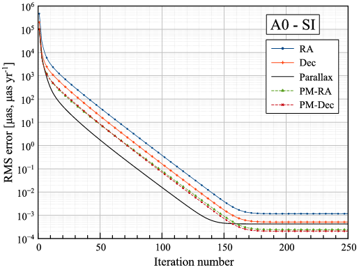
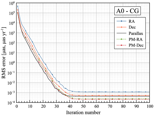
Figure 1: Convergence plots for test case A0 (without observation noise), using the simple iteration scheme (SI, left diagrams), and the conjugate gradient scheme (CG, right diagrams). The top diagrams show the RMS errors of the astrometric parameter (i.e., the RMS differences between the calculated and true values). The bottom diagrams show the RMS updates of the astrometric parameters.

To illustrate the convergence of the different iteration schemes, we use three kinds of diagrams, which are briefly explained hereafter.

Convergence plots show scalar quantities such as the RMS values of the errors, updates or residuals, plotted on a logarithmic scale versus the iteration number ($k$). For the error ($\@vec{e}_{k}$) and update ($\@vec{d}_{k}$) vectors we consider only the source parameters; the attitude errors and updates follow similar curves, not adding much information about the convergence behaviour. The source parameters are separated according to type ($\alpha*$, $\delta$, $\varpi$, $\mu_{\alpha*}$, and $\mu_{\delta}$). The purpose of these plots is to show the rate of global convergence of the different algorithms.

Error maps show, for selected iterations, the error in one of the astrometric parameters (i.e., its currently estimated value minus the true value) as a function of position on the celestial sphere. The purpose of these plots is to show graphically the possible existence of systematic errors in the solution as a function of position on the sky. Significant such errors could exist without being noticeable in the global convergence plots. To produce these error maps, the sky is divided into small bins of roughly equal solid angle, and the median error is computed over all the stars belonging to the bin. A colour is attributed to each bin according to the median error, and a map is plotted in equatorial coordinates, using an equal-area Hammer–Aitoff projection. In the maps shown, the sky is divided into 12 288 bins of approximately $1.8^{\circ}$ side length; there are on average 8.1 stars per bin. We choose to show only the distribution of parallax errors, although qualitatively similar maps are obtained for each of the five astrometric parameters.

Truncation error maps are similar to the error maps, but show the difference between the current iteration and the final (converged) iteration. They therefore display the type of systematic errors that could exist in the solution, if the iteration process is prematurely terminated.

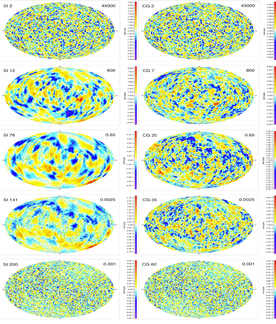
Figure 2: Parallax error maps for test case A0 (no observation noise) at selected points in the simple iteration scheme (SI, left column) and conjugate gradient scheme (CG, right column). The iteration number is shown in the top left corner of each map (the initial values are iteration 2 due to the ‘start-up’ procedure described in the text). The number in the top right corner is the approximate amplitude (in $\mu$as) of the colour scale. Starting from identical initial values of the astrometric parameters, SI and CG converge to the same solution (equal to the true parallaxes to within $\pm 0.001\leavevmode\nobreak\ \mu$as), although along different paths; moreover CG converges about four times quicker.

4.2 Case A: Uniform distribution of sources and weights

In Case A we consider a sky of isotropically distributed sources of uniform brightness, so that they all obtain the same statistical weight per observation. This weight corresponds to a standard deviation of 100 $\mu$as for the along-scan (AL) observations and 600 $\mu$as for the across-scan (AL) observations. These numbers are representative for Gaia’s expected performance for bright stars ($G$ magnitude from $\simeq 6$ to 13). The top diagrams in Fig. 2 show the distribution of initial parallax errors on the sky; the amplitude of these errors is about $\pm 45$ mas.

Three separate tests, subsequently denoted A0, A1, and A2, were made with the uniform source distribution in Case A:

A0:

No observational errors were added to the computed observations. Consequently both the SI and the CG should converge to the true source parameters.

A1:

Random centred Gaussian errors were added to the computed observations, with standard deviations equal to the nominal standard errors (100 and 600 $\mu$as AL and AC). Again, both SI and CG should converge to the same source parameters, which however will differ from the true values by several $\mu$as due to the observation noise.

A2:

This test used exactly the same noisy observations as A1, but the iterations start with a different set of initial values. After convergence, the solution should be exactly the same as in A1. This test was only made with the CG algorithm.

In all cases the Gauss–Seidel preconditioner (Algorithm 2) was used for both the SI and CG schemes. We have also tested the symmetric Gauss–Seidel preconditioner (Algorithm 3) on a smaller version ($S=0.01$) of this problem, but without any significant improvement in the convergence over the (non-symmetric) Gauss–Seidel preconditioner.

    

    

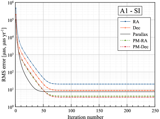
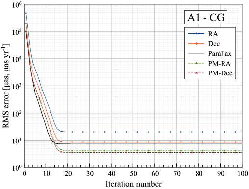
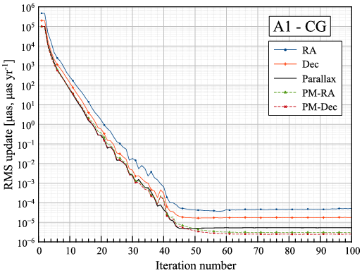
Figure 3: Convergence plots for test case A1 (including observation noise), using the simple iteration scheme (SI, left diagrams), and the conjugate gradient scheme (CG, right diagrams). See Fig. 1 for further explanation.

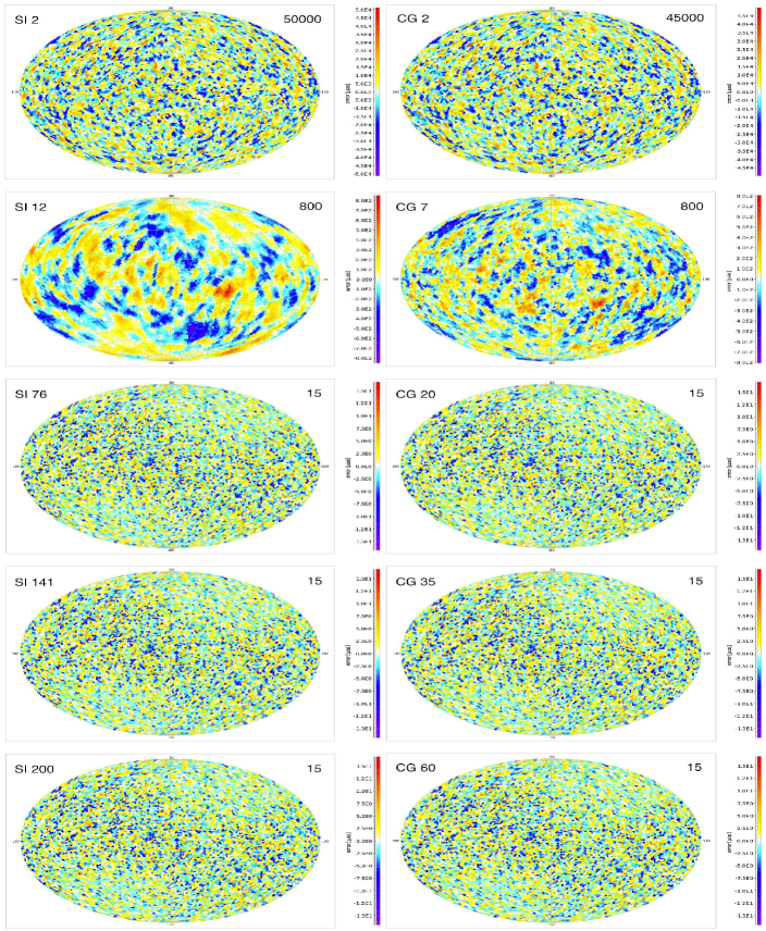
Figure 4: Error maps for test case A1 (including observation noise) at selected points in the simple iteration scheme (SI, left column) and conjugate gradient scheme (CG, right column). See Fig. 2 for further explanation of the diagram layout. Starting from identical initial parallax values, SI and CG converge to the same solution, although along different paths. Apparently, the parallaxes have converged more or less to their final values after iteration 76 (SI) or 20 (CG), but as shown in Fig. 5 there are then still significant, spatially correlated truncation errors that require many more iterations to be completely removed.

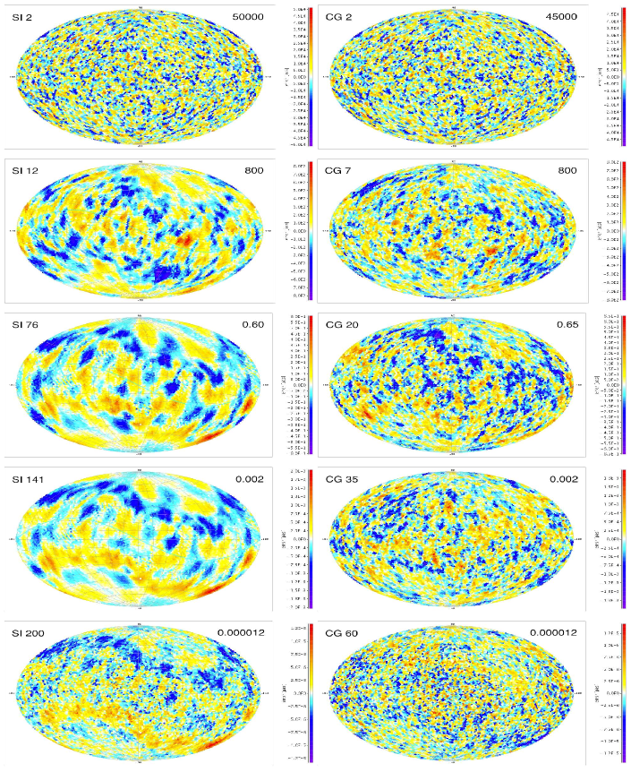
Figure 5: Truncation error maps for test case A1 at selected points in the simple iteration scheme (SI, left column) and conjugate gradient scheme (CG, right column). See Fig. 2 for further explanation of the diagram layout. Each map shows the difference between the result in the current iteration and the (presumably converged) solution obtained after 250 (SI) or 100 (CG) iterations. Although the parallaxes have converged more or less to their final values after iteration 76 (SI) or 20 (CG), as shown in Fig. 4, there are then still spatially correlated truncation errors at the $\pm 0.6\leavevmode\nobreak\ \mu$as level in both solutions.

4.2.1 Test case A0: Comparing SI and CG without noise

Figure 1 shows the global convergence for test case A0, i.e., without observation noise. The top diagrams show the errors of the astrometric parameters, and the bottom diagrams the updates. The left diagrams are for the SI scheme, and the right diagrams for CG. The errors and updates are expressed in $\mu$as (for $\alpha*$, $\delta$, and $\varpi$) and $\mu$as yr^-1 (for $\mu_{\alpha*}$ and $\mu_{\delta}$).

From Fig. 1 it is seen that both algorithms eventually reach the same level of RMS errors ($\la 0.001\leavevmode\nobreak\ \mu$as in position and parallax and $\la 0.001\leavevmode\nobreak\ \mu$as yr^-1 in proper motion), and that the updates settle at levels that are 1–2 dex below the errors. The updates do not systematically decrease beyond iteration $\sim\!200$ (SI) and $\sim\!60$ (CG), suggesting that the full numerical precision has been reached at these points.

The maps of parallax errors at selected iterations of test case A0 are shown in Fig. 2. The top maps show the initial errors (which are the same for SI and CG) and the bottom maps show the (apparently) converged results in iteration 200 (SI) and 60 (CG), respectively. The selection of intermediate results, although somewhat arbitrary, was made at comparable levels of truncation errors in the two algorithms. It is noted that CG converges three to four times faster than SI, in terms of the number of iterations required to reach a given level of truncation errors. Furthermore, it is seen that the converged error maps look quite identical. Inspection of the numerical results shows that this is indeed the case: whereas the RMS parallax error is $4.24\times 10^{-4}\leavevmode\nobreak\ \mu$as both in SI (iteration 200) and CG (iteration 60), the RMS value of the difference between the two sets of parallaxes is only $5.33\times 10^{-6}\leavevmode\nobreak\ \mu$as. This means that both algorithms have found virtually exactly the same solution, although one that deviates slightly from the true one.

The likely cause of this deviation is quantization noise when computing the observation times in the AGISLab simulations, as shown by the following considerations. Because double-precision arithmetic is not accurate enough to represent the observation times over several years, they are instead expressed in nano-seconds (ns) and stored as long (64 bit) integers. In the present simulations, which use a scaling factor $S=0.1$ (see Sect. 4.1), the satellite spin rate is about 19 arcsec s^-1, and the least significant bit of the stored observation times therefore corresponds to $0.019\leavevmode\nobreak\ \mu$as. This generates a (uniformly distributed) observation noise with an RMS value of $0.019\times 12^{-1/2}=0.0055\leavevmode\nobreak\ \mu$as. In order to estimate the corresponding parallax errors, we note that the ratio of the RMS parallax errors to the RMS observation noise depends only on the mean number of observations per source and on certain temporal and geometrical factors related to the scanning law, and is therefore invariant to a scaling of the observation noise. The ratio can be estimated from the A1 tests discussed in Sect. 4.2.2, which use an observation noise of $100\leavevmode\nobreak\ \mu$as and give an RMS parallax error of $7.26\leavevmode\nobreak\ \mu$as. The expected RMS parallax error due to the quantization of the observation times is then $0.0726\times 0.0055=0.00040\leavevmode\nobreak\ \mu$as, in fair agreement with the parallax errors of the ‘noiseless’ A0 tests.

Returning to the error maps in Fig. 2, a further observation is that the SI rather quickly develops a certain error pattern (most clearly seen in the map designated SI 76), correlated over some 10–20^∘, which only slowly fades away with more iterations, until it completely disappears. This can be understood in relation to the iteration matrix mentioned in Sect. 2.1: the dominant pattern shows the eigenvector corresponding to the largest eigenvalue of the iteration matrix. This is consistent with the very straight lines in the left diagrams of Fig. 1 between iterations $\sim\,$50 and 120, showing a geometric progression with a factor 0.91 improvement between successive iterations; we interpret this as $|\lambda_{\text{max}}|\simeq 0.91$. By contrast, the error maps for the CG scheme do not exhibit similar persistent patterns, have a smaller correlation length, and the convergence is only very roughly geometric and not even monotonic at all times.

4.2.2 Test case A1: Comparing SI and CG with noise

Figures 3 and 4 show the corresponding convergence plots and error maps for test case A1, where the simulated observations include a nominal noise. The convergence plots (Fig. 3) show that the RMS errors have already settled in iteration 70 (SI) or 20 (CG), at which points the solutions are however far from converged, as shown by the RMS updates in the lower diagrams. The full convergence is only reached at iteration 200 (SI) or 60 (CG), exactly as in the noiseless case (A0). The updates then settle at about the same levels as in case A0. The rate of convergence is therefore not significantly affected by the noise (if anything, the noise seems to have a slightly stabilizing effect in the final iterations before convergence).

The error maps (Fig. 4) start, in the top diagrams, at the same initial approximation in case A0, and develop along different paths to the converged solutions in the bottom diagrams, which are virtually identical for SI and CG. Inspection of the numerical results confirms that the two algorithms have indeed converged to the same solution, within the rounding errors: for example, the RMS values of the parallax error in SI (iteration 200) and CG (iteration 60) are both $7.26\leavevmode\nobreak\ \mu$as, while the RMS difference between the solutions is $5.16\times 10^{-6}\leavevmode\nobreak\ \mu$as.

Although the error maps in Fig. 4 do not appear to change much after iteration 76 (SI) and 20 (CG), we inferred from the convergence plots that neither solution was truly converged at these points. In order to examine the evolution of the errors beyond these points, we show in Fig. 5 the truncation errors in parallax, i.e., the difference between the solution at a given iteration and the solution after the maximum number of iterations (250 for SI and 100 for CG). Interestingly, the truncation error maps in Fig. 5 look very much like the error maps in Fig. 2 for the noiseless case (A0). The iterations therefore follow more or less the same path through solution space, independent of the observation noise (but of course different in SI and CG). This is consistent with our previous observation that A0 and A1 require the same number of iterations for full convergence. – It is noted that the truncation errors for the SI in iteration 200 still show a residual pattern clearly related to the scanning law (with systematically negative and positive parallax errors around ecliptic latitude $+45^{\circ}$ and $-45^{\circ}$, respectively), although the amplitude is very small, about $\pm 5\times 10^{-6}\leavevmode\nobreak\ \mu$as. The truncation errors for the CG, at iteration 60, have a similar amplitude but are spatially less correlated.

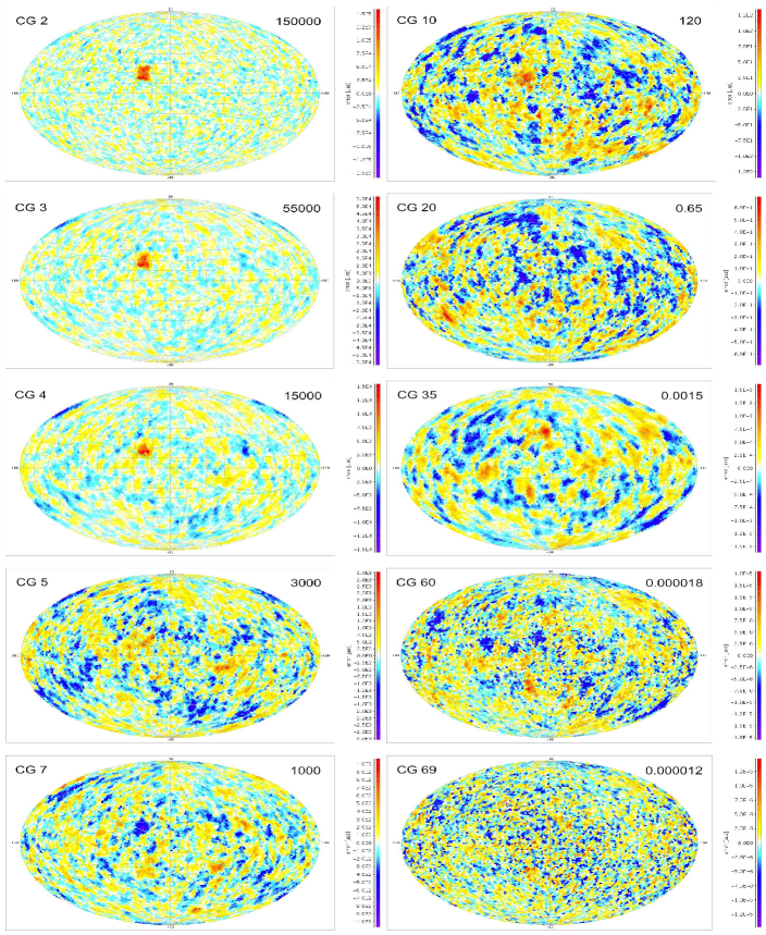
Figure 6: Truncation error maps for test case A2 (same as A1 but with different initial values) at selected iterations in the CG scheme. More of the first few iterations are shown in order to illustrate the diffusion of the large, localized initial errors. See Fig. 2 for further explanation of the diagram layout.

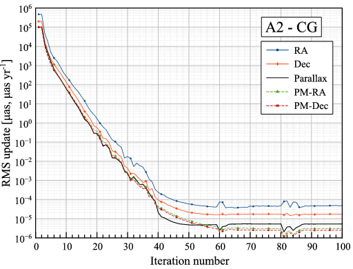
Figure 7: Convergence plots for test case A2 (same as A1 but with different initial values), using the conjugate gradient scheme (CG). See Fig. 1 for further explanation.

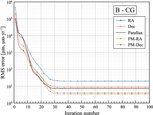
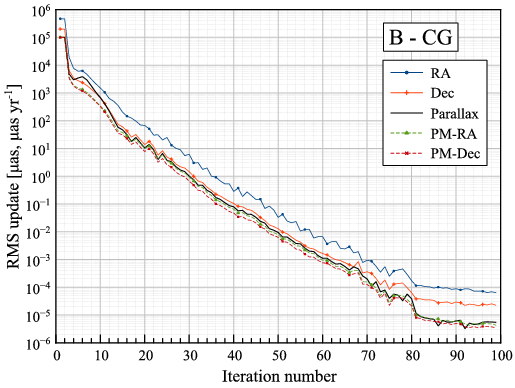
Figure 8: Convergence plots for test case B (non-uniform weight distribution), using the conjugate gradient scheme (CG). See Fig. 1 for further explanation.

4.2.3 Test case A2: Starting CG from a different point

The previous tests have all started from the same initial approximation, illustrated by the errors maps SI2 and CG2 at the top of Figs. 2 and 4. The aim of test case A2 is to show that the CG algorithm finds the same solution, for the same observations as in A1, when starting from a different initial approximation. To this end, we added 0.2 arcsec to the initial parallax values of 504 sources in an area of about $200\leavevmode\nobreak\ \text{deg}^{2}$ centred on $\alpha=30^{\circ}$, $\delta={+}20^{\circ}$; subsequently we refer to this as the ‘W area’. Having strongly deviating initial values in a relatively small area makes it easy to follow their diffusion among the sources in subsequent iterations, e.g., by visual inspection of the error maps (Fig. 6). A position close to the ecliptic was chosen for the W area, since the ecliptic region is less well observed by Gaia, due to its scanning law, than other parts of the celestial sphere. Potentially, therefore, the astrometric solution might be less efficient in eliminating the initial errors in such an area.

The convergence plots in Fig. 7 are not drastically different from the corresponding plots in test case A1 (right panels of Fig. 3), although the updates do not reduce quite as quickly after iteration $\sim\,$40. The truncation error maps in Fig. 6 show that the large initial errors in the W area are quickly damped in the first few iterations, and even reversing the sign around iteration 7; after iteration 10 the W area does not stand out. The subsequent truncation errors maps (e.g., in iteration 20 and 35) are remarkably similar to those in test case A1 (right panels of Fig. 4). However, the residual large-scale truncation patterns do not completely disappear, to the same level as in A1, until around iteration 69.

Numerically, the RMS parallax difference between the A2 and A1 solutions is $4.95\times 10^{-6}\leavevmode\nobreak\ \mu$as in iteration 60, and $4.64\times 10^{-6}\leavevmode\nobreak\ \mu$as in iteration 69. Comparing only the parallaxes for the 504 sources in the W area, the RMS difference is $5.74\times 10^{-6}\leavevmode\nobreak\ \mu$as. The converged results are thus virtually identical; in particular the initial offsets in the W area have been reduced by more than 10 orders of magnitude.

4.3 Case B: Non-uniform distribution of weights

The uniform sky considered in Case A is highly idealised: the real sky contains a very non-uniform distribution of stars of different magnitudes. The standard deviation of the along-scan observation noise, $\sigma$, is mainly a function of stellar magnitude, and could vary by more than a factor 50 between the bright and faint sources. As a result, the statistical weight of the observations (defined as the sum of $\sigma^{-2}$ for the observations collected in a time interval of a few seconds) is often very different in the two fields of view. This happens, for example, when one field of view is near the galactic plane and the other is at a high galactic latitude, or when a rich and bright stellar cluster passes through one of the fields. At such times the along-scan attitude is almost entirely determined by the observations in the field with the higher weight. Intuitively it would seem that this could weaken the connectivity between the fields, and consequently the quality of the astrometric solution. A particular concern could be that the accuracy of the absolute parallaxes of the cluster stars, and their connection to the global reference frame, might suffer, since both these qualities critically depend on Gaia’s ability to measure long arcs by connecting observations in the two fields of view. In the new reduction of the Hipparcos data by van Leeuwen (2007) special attention was given to the weight distribution between the two fields of view when performing the attitude solution. As described in Sect. 10.5.3 of van Leeuwen (2007), the weight ratio was not allowed to exceed a certain factor ($\sim$3); this was achieved by reducing, when necessary, the weights of the observations in one of the fields. On the other hand, from a more theoretical standpoint it can be argued that the intentional removal or down-weighting of perfectly good data cannot possibly improve the results.

In order to investigate the impact of an inhomogeneous weight distribution on the solution, we present in Case B a sky with a strong and evident contrast in statistical weight. The same source distribution and initial values were used as in Case A2, but all the errors of the observations, as well as their assumed standard errors in the solution, were reduced by a factor 5 for the 504 sources in the W area (centred on $\alpha=30^{\circ}$, $\delta={+}20^{\circ}$). As before, the starting values of the parallaxes in the W area were also offset by 0.2 arcsec. This case could represent a situation where the stars in a single bright cluster obtain very accurate individual astrometric measurements, while the initial parallax knowledge of the cluster is strongly biased. In Case B we test the ability of the astrometric solution to produce unbiased parallax estimates for the cluster, as well as for the rest of the sky, without using any weight-balancing schemes such as outlined above. The observations are strictly weighted by $\sigma^{-2}$, so the weight contrast between the fields of view is roughly a factor 25 whenever the cluster stars are observed, while it is about 1 at all other times.

The convergence plots in Fig. 8 show that the CG scheme converges also in this case, albeit significantly slower than in Case A – about 95 iterations are needed instead of 60. The error maps, in the left column of Fig. 10, show the W area in stark contrast to the rest of the sky during the initial iterations. At iteration 20 the errors in the W area are still very significant, and have the opposite sign of their initial values. From iteration 35 and onwards, the errors in the W area are typically smaller than in the rest of the sky, and in iteration 60 the solution appears to have converged everywhere. However, as shown by the truncation error maps in the right column of Fig. 10, the errors in the W area continue to decrease at least up to iteration 90. We consider the solution converged from iteration 95, at which point the parallax updates in the W area are about $10^{-5}\leavevmode\nobreak\ \mu$as.

That the high contrast in weight between the W area and the rest of the sky in Case B has had no negative effect on the solution is more clearly seen in Table 1, which compares the average and RMS parallax errors, inside and outside of the W area, for the converged solutions in Case A1 and Case B. First of all it can be noted that the average parallax errors in all cases are insignificant, i.e., consistent with the given RMS errors and the assumption that the errors are unbiased. The slightly negative averages inside the W area and slightly positive averages in the rest of the sky are a random effect of the particular noise realization used in these tests, and cannot be interpreted as a bias. Secondly, it can be noted that both the average parallax error and the RMS parallax error inside the W area are reduced roughly in proportion to the observational errors (i.e., by a factor $\sim$5), while the errors outside of the W area are very little affected. This is just as expected in the ideal case that the weight contrast is correctly handled by the solution.

The test cases A1 and B use the same seed for the random observation errors, which therefore strictly differ by a factor 5 in the W area between the two cases. This allows a very detailed comparison of the results. For example, the marginally smaller RMS error outside of the W area in Case B ($7.25466\leavevmode\nobreak\ \mu$as) compared to Case A1 ($7.25570\leavevmode\nobreak\ \mu$as) is probably real and reflects the improved attitude determination in Case B (thanks to the more accurate observations in the W area), which benefits also some sources that are not in the W area. Figure 9 is a comparison of the individual parallax errors in the W area from the two solutions. The diagonal line has a slope of 0.2, equal to the ratio of the observation errors in the W area between Case B and Case A1. The diagram suggests that, to a good accuracy, the final parallax errors scale linearly with the corresponding observation errors.

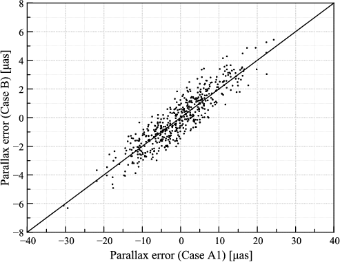
Figure 9: Comparison of the individual parallax errors of the 504 sources in the W area, from the solution in Case A1 (horizontal axis) and Case B (vertical axis).

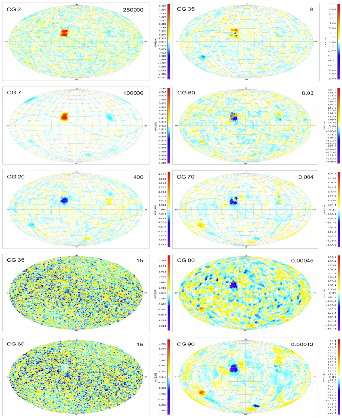
Figure 10: Parallax errors and truncation errors for test case B (non-uniform weight distribution). The error maps in the left column show the differences between the parallax values in selected iterations and their true values. The truncation error maps in the right column show the difference between the parallax values in selected iterations and the converged values (in iteration 100). See Fig. 2 for further explanation of the diagram layout.

Table 1: Average and RMS parallax errors in Case A1 (where all observations have the same standard deviation) and Case B (where the observations in the W area have a factor 5 smaller noise). The numbers following the $\pm$ symbol are the RMS parallax errors. All errors are expressed in $\mu$as.

Solution	W area	non-W area
	(504 sources)	(99 496 sources)
Case A1 (CG 60)	$-0.45046\pm 8.33135$	$+0.01341\pm 7.25570$
Case B (CG 95)	$-0.06747\pm 1.88051$	$+0.01419\pm 7.25466$

4.4 Definition of a convergence criterion

The iteration loops in the SI and CG schemes are set to run for a given number of iterations. We now turn to the question how to define a convergence criterion, i.e., to determine when to stop the iterations.

In standard implementations of the CG algorithm it is customary to stop iterating when the norm of the residual vector $\@vec{r}=\@vec{b}-\@vec{N}\@vec{x}$ is less than some pre-defined small fraction $\varepsilon$ of the norm of $\@vec{b}$ (e.g., Golub & van Loan 1996). The tolerance $\varepsilon$ must not be smaller than the unit roundoff error of the floating point arithmetic used ($2^{-52}\simeq 2\times 10^{-16}$ in our case, using double precision), but in practice it may have to be many times larger in order to accommodate the accumulated roundoff errors when computing the residual vector. This is especially the case when the number of unknowns is very large, as in the present application. The choice of $\varepsilon$ is therefore not trivial: a slightly too small value would not terminate the iterations, while a slightly too large value may, as we have seen, result in undesirable truncation errors. Ideally we want a convergence criterion that effectively ensures that we have reached the full accuracy permitted by the finite-precision arithmetic.

In this context it is worth pointing out that AGIS is only one step of Gaia’s data reduction, and that AGIS will be run many times during the data reduction process. Indeed the output from AGIS will be used to improve other calibration processes (line spread functions, photometry, etc.) which in turn can be used to improve the astrometric solution. Since AGIS is thus part of an outer iteration loop involving several other calibration processes, it may not be useful to enforce a very strict convergence criterion for AGIS until at the very last few outer iterations. In other words, as long as the other calibrations are not well settled, we can live with slightly non-converged astrometric solutions. In the final outer iteration, the astrometric solution should be driven to the point where the updates are completely dominated by numerical noise. The criteria discussed here have that aim. We consider in the following only the CG scheme because of its superior convergence properties.

In the previous analysis we have studied the convergence in terms of the updates $\@vec{d}_{k}$, error vectors $\@vec{e}_{k}$, and truncation errors $\@vec{\epsilon}_{k}$. The error vectors are of course not known for the real mission data, and the truncation errors only become known after having made many more iterations than strictly necessary, and are therefore not useful in practice. The convergence criterion could however be based on the updates or various other quantities defined in terms of the design equation residuals $\@vec{s}_{k}$ or normal equation residuals $\@vec{r}_{k}$ (cf. Sect. 2).

Based primarily on a visual inspection of the various diagrams, including the convergence plots (Figs. 1, 3, 7, 8) and the parallax truncation errors maps (Figs. 5, 6, 10), it was concluded that about 60, 60, 69 and 95 iterations were required for full convergence of the CG scheme in the four test cases A0, A1, A2 and B. An ideal convergence criterion should tell us to stop at about these points, and it should also be robust against changes in the number of sources, their distribution on the celestial sphere, and the weight distribution of the observations. It is not possible to explore the robustness issue in this paper, and we therefore concentrate on finding some plausible candidate criteria.

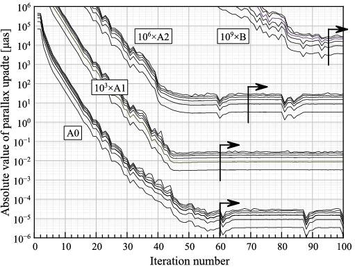
Figure 11: Statistics of the parallax updates for the CG solutions in Case A0, A1, A2 and B. In each Case the fives curves show, from bottom up, the quantiles $q_{0.5}$ (median), $q_{0.9}$, $q_{0.99}$, $q_{0.999}$, and $q_{0.9999}$ of the absolute values of the parallax updates in each iteration. The thick vertical lines with arrows indicate the iterations where the solutions had effectively converged according to the truncation errors maps. For better visibility the curves in Case A1, A2 and B have been shifted upwards by 3, 6 and 9 dex, respectively.

4.4.1 Criteria based on the parallax updates

Among the five astrometric parameters, the parallaxes are especially useful for monitoring purposes, because they are not affected by a possible frame rotation between successive iterations. It would therefore seem natural to define a convergence criterion in terms of some statistic of the parallax updates. In the convergence plots we have plotted the RMS value of the updates. However, it is possible that the updates for a small fraction of the sources (e.g., those with high statistical weights as in the W area of Case B) converges less rapidly than the bulk of the sources, and that the overall standard width of the updates is therefore not the best indicator. Instead we will consider quantiles of the absolute values of the parallax updates such as $q_{0.999}$ (that is, 99.9% of the absolute updates are less than $q_{0.999}$).

Figure 11 summarises the evolution of selected quantiles of the absolute parallax updates for the CG solutions in the four test cases. The arrows indicate the first converged iterations according to the previous discussion. In all cases, the parallax updates eventually reach a final level, e.g., $\simeq 2\times 10^{-5}\leavevmode\nobreak\ \mu$as for $q_{0.999}$. Remarkably, however, at least in Case A1 and A2 this level is reached well before convergence (e.g., at iteration 45 in Case A1 and 50 in Case A2). At these points, the truncation error maps still contain significant large-scale features with amplitudes of about $5\times 10^{-5}\leavevmode\nobreak\ \mu$as (Fig. 12). The same conclusion is reached whatever quantile is considered. It thus appears that the parallax updates alone are not sufficient to define a criterion for the full convergence. On the other hand, it appears that the magnitude of the updates, before they have reached their final levels, gives a good indication of the magnitude of the truncation errors at that point.

       

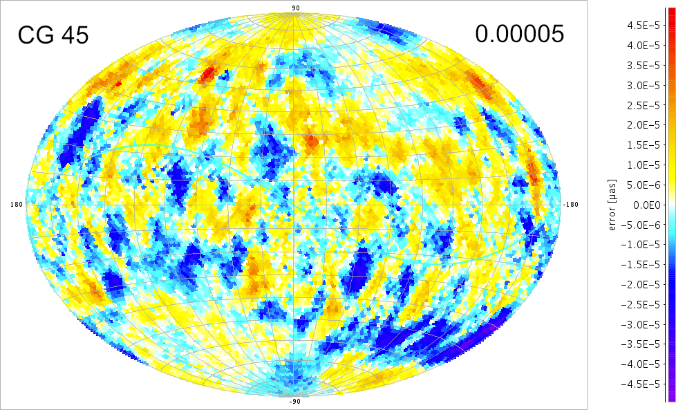
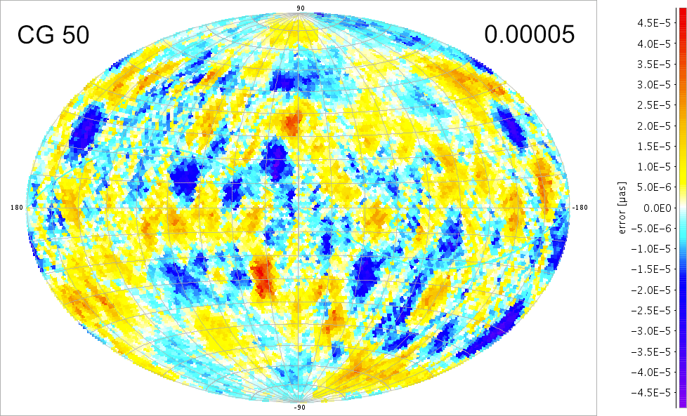
Figure 12: Truncation error maps for iteration 45 of Case A1 (left) and iteration 50 of Case A2 (right). At these points the parallax updates have reached their final levels according to Fig. 11, but these maps show that the solutions are not quite converged.

    

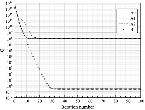
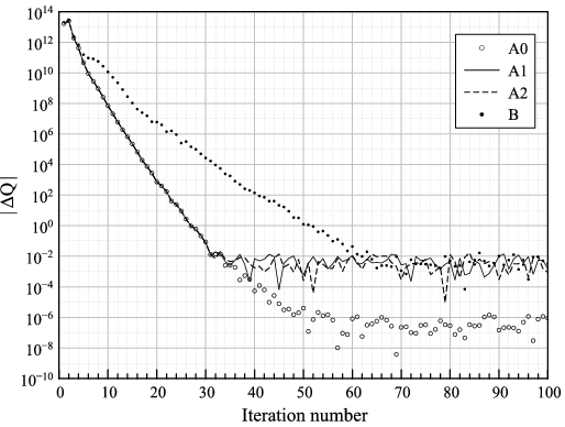
Figure 13: Left: Evolution of $Q_{k}=\|\@vec{s}_{k}\|^{2}$ for the CG solutions in Case A0, A1, A2 and B. Right: Evolution of the absolute value of $\Delta Q_{k}=Q_{k-1}-Q_{k}$ for the same solutions.

    

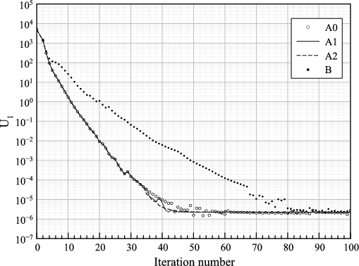
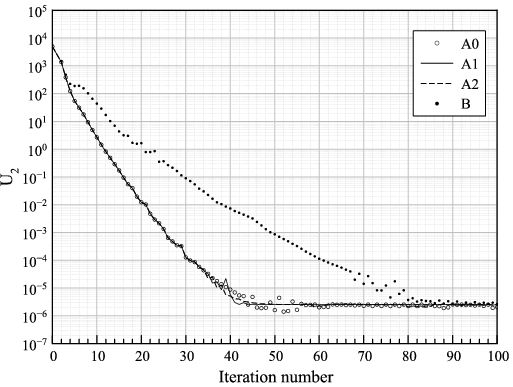
Figure 14: Left: Evolution of $U_{1}=(\rho_{k}/n)^{1/2}$ for the CG solutions in the four test cases. Right: Evolution of $U_{2}=(\alpha_{k}\rho_{k}/n)^{1/2}$ for the same solutions.

    

    

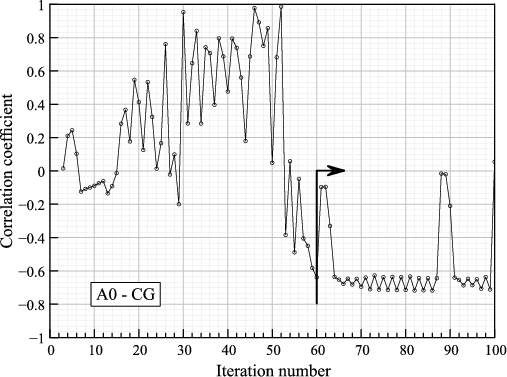
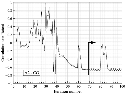
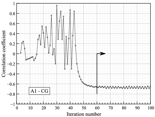
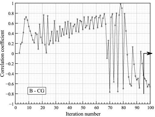
Figure 15: Correlation coefficient $R_{k}$ between successive parallax updates of the CG solutions in Case A0, A1, A2 and B. The thick vertical lines with arrows indicate the iterations where the solutions had effectively converged according to the truncation errors maps.

4.4.2 Criteria based on residual vector norms

Independent of the kernel and iteration schemes, we know for each iteration the three vectors $\@vec{d}_{k}$ (updates), $\@vec{s}_{k}$ (design equation residuals), and $\@vec{r}_{k}$ (normal equation residuals). There are a number of different vector norms that can be computed from these, taking into account different possible metrics. Ideally, we are looking for a single scalar quantity that is theoretically known to decrease as long as the solution improves.

In the CG scheme the square of the norm of the design equation residuals, $Q_{k}=\|\@vec{s}_{k}\|^{2}$, should be non-increasing according to Eq. (6). After convergence, it is expected to reach a value of the order of $\nu=m-n$, where $m$ is the number of observations and $n$ the number of unknowns. In our (small-scale) test cases we have $\nu\sim 10^{8}$. Figure 13 (left) shows that the test cases that contain observation noise (A1, A2 and B) reach this level in some 15–25 iterations; in the noise-less case (A0) a much lower plateau is reached in about 30 iterations. Although not visible in the left diagram, $Q_{k}$ continues to decrease for many more iterations, as shown in the right diagram of Fig. 13, where the absolute values of $\Delta Q_{k}=Q_{k}-Q_{k-1}$ are plotted for the same solutions. Unfortunately these values seem to reach a stable level even before the updates. The design equation residuals therefore do not provide a useful convergence criterion.

There is no guarantee that the norms of $\@vec{d}_{k}$ and $\@vec{r}_{k}$ decrease monotonically, although in the SI scheme they behave asymptotically as described in Sect. 2.1 (exponential decay). The same statements can be made for the scalar product

$$\rho_{k}=\@vec{r}_{k}^{\prime}\@vec{d}_{k}=\@vec{d}_{k}^{\prime}\@vec{K}\@vec{d}_{k}=\@vec{r}_{k}^{\prime}\@vec{K}^{-1}\@vec{r}_{k}\,,$$ (19)

which is non-negative for any positive-definite preconditioner $\@vec{K}$, and has the advantage of being dimensionless. Since the quadratic form in Eq. (19) implies a sum over all $n$ parameters, we define the RMS-type quantity $U_{1}\equiv(\rho_{k}/n)^{1/2}$, which is plotted in Fig. 14 (left).

For the CG scheme we note that $\rho_{k}$ is already calculated as part of Algorithm 5). An even more relevant quantity could be

$$\@vec{d}_{k}^{\prime}\@vec{N}\@vec{d}_{k}=\alpha_{k}^{2}\@vec{p}_{k}^{\prime}\@vec{N}\@vec{p}_{k}=\alpha_{k}\rho_{k}\,,$$ (20)

which according to Eq. (6) is the amount by which the sum of squared residuals $Q\equiv\|\@vec{s}\|^{2}$ is expected to decrease in the next iteration (mathematically, therefore, $\alpha_{k}\rho_{k}=\Delta Q_{k+1}$). Since $\@vec{N}$ is the inverse of the formal covariance of the parameters, $U_{2}\equiv(\alpha_{k}\rho_{k}/n)^{1/2}$ has a simple interpretation: it is the RMS update defined in units of the statistical errors.

Figure 14 shows the evolution of $U_{1}$ and $U_{2}$ for the CG solutions in the four test cases. There is in practice little difference between $U_{1}$ and $U_{2}$, which merely reflects the circumstance that $\alpha_{k}$ is of the order of unity throughout the CG iterations. Moreover, the plots in Fig. 14 are are quite similar to those of the parallax updates in Fig. 11, and therefore no more useful for defining a convergence criterion.

4.4.3 Criteria based on the correlation of successive updates

The conclusion from preceding sections is that various simple statistics based on the updates and/or residuals of the current iteration are insufficient to indicate that the solution has reached full numerical accuracy. In particular, none of the above criteria indicate the need to continue iterating after iteration 45 in Case A1, and 50 in Case A2. Yet, inspection of the truncation errors maps in Fig. 12 clearly shows the need for additional iterations. The truncation errors in the subsequent iterations tend to be similar, only with reduced amplitude. This can perhaps be understood as a consequence of the frequent reinitialisation of the CG algorithm in this regime. In the limit of constant reinitialisation, Algorithm 5 becomes equivalent to the SI scheme (Algorithm 4), in which the truncation errors tend to decay exponentially. In this situation the updates also decay exponentially, and therefore have a strong positive correlation from one iteration to the next. This suggests that we should look at the correlation between the updates in successive iterations as a possible convergence criterion.

Figure 15 shows the evolution of the correlation coefficient between successive parallax updates $\@vec{\delta\varpi}_{k}$,

$$R_{k}=\frac{{\@vec{\delta\varpi}_{k}}^{\prime}{\@vec{\delta\varpi}_{k-1}}}{({\@vec{\delta\varpi}_{k}}^{\prime}{\@vec{\delta\varpi}_{k}})^{1/2}({\@vec{\delta\varpi}_{k-1}}^{\prime}{\@vec{\delta\varpi}_{k-1}})^{1/2}}\,,$$ (21)

in the four solutions. As in Fig. 11, the arrows indicate the points where convergence had been reached according to the discussion above. It is seen that $R_{k}$ changes from predominantly positive to predominantly negative values roughly at the points when the parallax updates (Fig. 11) or $U_{1}$ and $U_{2}$ (Fig. 14) reach their minimum values set by the numerical noise. Significantly, however, $R_{k}$ continues to decrease beyond these points, reaching a roughly constant level $R\simeq-0.67$ at the point of convergence.

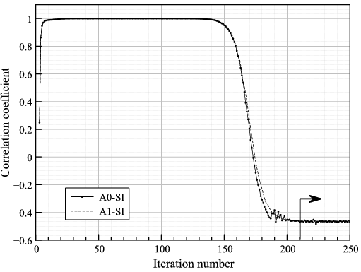
Figure 16: Correlation coefficient between successive parallax updates of the SI solutions in Case A0 and A1. The thick vertical line with an arrow indicates where the solutions had effectively converged according to the truncation errors maps.

As already mentioned, the CG scheme more or less reverts to the SI scheme in the final iterations, due to the frequent reinitialisations. However, the evolution of the correlation coefficient in Fig. 15 is partly obscured by the irregularity of the reinitialisations – for example, the sudden rise in $R_{k}$ at iteration 60 and 81 in Case A2, and at iteration 87 and 93 in Case B, seem to be related to the fact that no reinitialisation occurred two iterations earlier (while otherwise reinitialisation was the rule in this regime). For comparison we show in Fig. 16 the evolution of $R_{k}$ in the SI scheme applied to Case A0 and A1. Here the behaviour is much more regular, and the correlation coefficient reaches a stable value of $\simeq-0.47$ from iteration 210, at which point the solutions had converged according to Figs. 1 and 3.

4.4.4 Conclusion concerning convergence criteria

The previous discussion shows how difficult it is to define a reliable convergence criterion that is sufficiently strict according to our aims. Fortunately, as already pointed out, full numerical convergence is only required in the very final outer processing loop (which includes many other processes apart from the final astrometric core solution). For that purpose a combination of the above criteria might be appropriate, i.e., requiring numerically small updates combined with a correlation coefficient that has settled to some negative value. In any case it will be wise to carry out a few extra iterations after the formal criterion has been met.

For the provisional astrometric solutions, where full numerical convergence is not required, it will be sufficient to stop the CG iterations when the RMS parallax update or some residual norm such as $U_{1}$ or $U_{2}$ is below some fixed tolerance (of the order of $0.01\leavevmode\nobreak\ \mu$as and $10^{-3}$, respectively).

5 CG implementation status in AGIS

The AGISLab results presented in this paper, as well as numerous other experiments covering a range of different input scenarios (number of stars, initial noise level of the unknowns, etc.) convincingly demonstrate the general superiority of the CG scheme over SI in terms of convergence rate and its ability to more quickly remove correlated errors from the solution. This practical confirmation of the theoretical arguments (Sect. 2.1 and 2.2) was an important pre-requisite for supporting CG also in the AGIS framework. This has been done by now, such that both the SI and CG scheme are available in AGIS with the same functionality and fidelity as in AGISLab.

The implementation of the core CG scheme is rigorously equivalent to Algorithm 5 with small but conceptually irrelevant modifications to better match the existing way of how the iterations are organized in AGIS. The same is true for the Gauss–Seidel preconditioner kernel. The concrete accumulation of design equations is done somewhat differently to how it is specified in Algorithm 2, however, the resulting normal equations of the preconditioner $\@vec{K}_{2}$ in Eq. (14), viz. $\@vec{N}_{s}$ (actually one per source) and $\@vec{N}_{a}$ are again strictly equivalent to what a faithful implementation of the algorithm, as in AGISLab, yields.

The algorithms in this paper implicitly assume an underlying all-in-memory software design which is true for AGISLab but not for AGIS. Owing to the large data volumes that will have to be processed for the real Gaia mission (Sect. 4.1) AGIS is by necessity a distributed system (O’Mullane et al. 2011) capable of executing parallel processing threads on a large number (hundreds to thousands) of independent CPU cores. As an example, the accumulation of source and attitude normal equations is done in different processes running on different CPUs. Hence, the loop in lines 12–14 of Algorithm 2, which adds the contribution of all observations of source $i$ to the attitude normal equations, cannot be done directly in the same process that treats source $i$. This complicates matters considerably and, inevitably, leads to different realizations of CG in AGIS and AGISLab.

Extensive comparisons between AGIS and AGISLab were performed to ensure the mathematical and numerical equivalence and correctness of the two implementations. The tests in AGIS were done using a simulated data set with 250 000 stars isotropically distributed across the sky and very conservative starting conditions for the unknowns with random and systematic errors of several 10 mas. A comparable configuration (scaling factor $S$, etc.) was chosen for AGISLab.

The AGIS results fully confirmed all findings of Sect. 4.2, notably the important point that CG and SI converge to solutions which are identical to within the expected numerical limits. Moreover, a direct comparison of various key parameters as a function of iteration number, e.g., astrometric source and attitude parameter errors and updates, solution scalars of CG like $\alpha$, $\beta$, and $\rho$ (see Algorithm 5), showed a satisfying agreement between corresponding AGIS and AGISLab runs. Remaining differences are at the level of 1 iteration (e.g., the parallax error reached in AGISLab in iteration $k$ is reached or surpassed in AGIS not later than in iteration $k+1$ for all values of $k$), and have been attributed to not using exactly the same input data (AGISLab uses an internal on-the-fly simulator). This successfully concluded the validation of the CG implementation in AGIS.

It is clearly expedient to employ CG as much as possible; however, in practice with the real mission data we anticipate that a hybrid scheme consisting of alternating phases of SI and CG iterations will be needed. The reason is the necessity to identify and reject outlier observations which is a complex process done through observation weighting in AGIS. As long as the solution has not converged, these weights vary from one iteration to the next, which means that a slightly different least-squares problem is solved in every iteration. While this has no negative impact on the very robust SI method, we have observed that it does not work at all in the case of CG. This is not surprising and in fact expected as the changing weights lead to a violation of the conjugacy constraint (see Sect. 2.2) which is crucial for CG. Hence, we are envisaging a mode in which AGIS starts with SI iterations up to a point where the weights have stabilized to a given degree, then activate CG, followed by perhaps another SI phase to refine the weights further, then again CG, etc. This will probably make the automatic reinitialization of CG obsolete. The hybrid SI–CG scheme is a further development step in AGIS, and a more detailed discussion of relevant aspects and results is deferred to a future paper.

6 Conclusion

We have shown how the conjugate gradient algorithm, with a Gauss–Seidel type preconditioner, can be efficiently implemented within the already existing processing framework for Gaia’s Astrometric Global Iterative Solution (AGIS). This framework was originally designed to solve the astrometric least-squares problem for Gaia using the so-called Simple Iteration (SI) scheme, which is intuitively straightforward but computationally inefficient. The conjugate gradient (CG) scheme, by using the same kernel operations as SI, takes about the same processing time per iteration but requires a factor 3–4 fewer iterations. Both schemes have been extensively tested using the AGISLab test bed, which allows to perform scaled-down and simplified simulations of Gaia’s astrometric observations and the associated least-squares solution, using (in our case) $10^{5}$ sources and a total of about 2 million source and attitude unknowns.

To within the numerical noise of the double-precision arithmetic, corresponding to $<10^{-5}\leavevmode\nobreak\ \mu$as in parallax, the SI and CG schemes converge to identical solutions. In the case when no observational noise was added to the simulated observations, the solutions agree with the true values of the astrometric parameters to within the numerical noise. Thus we conclude that the iterative method provides the correct solution to the least-squares problem, provided that a sufficient number of iterations is used (full numerical convergence reached). As theoretically expected, the resulting solution is completely insensitive to the initial values of the astrometric parameters, although the rate of convergence may depend on the initial errors.

Although the SI and CG schemes eventually reach the same solution, to within the numerical precision of the computations, the truncation errors obtained by prematurely stopping the iteration have quite different character in the two schemes. In the SI scheme the truncation error maps are often strongly correlated over large parts of the celestial sphere, while in the CG scheme there is less spatial correlation. Thus, the CG scheme not only converges faster than SI, but the truncation errors at a given level of the updates are considerably more ‘benign’ in terms of large-scale systematics.

Most of the numerical experiments use a highly idealised, uniform distribution of sources, and a uniform level of the standard error of the observations. However, it has been demonstrated that the solution works flawlessly also in the case when the observations have a much larger weight in a small part of the sky (representing, for example, a bright stellar cluster). Although such a situation needs more iterations, the converged solution correctly reflects the weight distribution of the observations – i.e., the accuracy of the astrometric parameters of the cluster stars is increased roughly in proportion to their increased observational accuracy, without any noticeable negative impact on the results for other stars.

We have stressed the need to drive the iterations to full numerical convergence, at least in the final astrometric solution for the Gaia catalogue. This is important in order to avoid that the final catalogue contains truncation errors that are unrelated to the mission and satellite itself, but merely caused by inadequate processing. Such truncation errors could mimic ‘systematic errors’ in the catalogue. The Gaia catalogue will certainly not be free of systematic errors, but at least we should insist that they are not produced by prematurely stopping the astrometric iterations. However, achieving full numerical convergence may require many iterations beyond the point where simple metrics indicate convergence. It is in fact quite difficult to define a numerically strict convergence criterion, although we have found that the correlation between updates in successive iterations may provide a useful clue. At the point where the updates have not yet settled at their final level, the magnitude of the updates gives a good indication of the remaining truncation errors. If one does not insist on full numerical convergence, it is therefore relatively safe to stop iterating when the updates have reached a sufficiently low level, say below 0.01 $\mu$as.

The CG algorithm described in this paper only considers the two major processing blocks in AGIS, namely the determination of the source and attitude parameters. This restriction was intentional, in order to simplify the description and numerical testing. At the same time, the successful disentangling of the source and attitude parameters is the key to a successful solution, as shown by numerous experiments. Nevertheless, the proposed algorithm is readily extended to the fully realistic problem that includes calibration and global parameters, and has in fact been realised in this form and successfully demonstrated in the current AGIS implementation at the Gaia data processing centre in ESAC (Madrid).

Our aim has been to investigate the applicability of the CG algorithm for solving Gaia’s astrometric least-squares problem efficiently within the AGIS framework. To this end we have considered a scaled-down and highly idealized version of the problem where many detailed complications in the real Gaia data are ignored. Nevertheless, within the given assumptions, we have successfully demonstrated how the CG algorithm can be adapted to the astrometric core solution. Moreover, by means of numerical simulations we have shown that the numerical accuracy achieved with this method is high enough that it will not be a limiting factor for the quality of the astrometric results.

Appendix A Efficiency of the least-squares method

This appendix reviews some important properties of the least-squares method, which motivate its present application.

The estimation problem associated with the astrometric core solution has the following characteristics: (i) within the expected size of the errors, it is completely linear in terms of the adjusted parameters or unknowns; (ii) the observational errors are unbiased, (iii) uncorrelated, and (iv) of known standard deviation. Property (i) follows from the small absolute sizes of the errors; (ii) assumes accurate modelling at all stages of the data analysis; (iii) follows from the Poissonian nature of the photon noise being by far the dominating noise source; and (iv) is ensured by the estimation method applied to the individual photon counts in the raw data. Dividing each observation equation by the known standard deviation of the observation error thus results in the standard linear model $\@vec{h}=\@vec{M}\@vec{x}+\@vec{\nu}$, where the vector of random observation noise $\@vec{\nu}$ has expectation $\text{E}(\@vec{\nu})=\@vec{0}$ and covariance $\text{E}(\@vec{\nu\nu^{\prime}})=\@vec{I}$. This is equivalent to the overdetermined set of design equations introduced in Sect. 2.

The Gauss–Markoff theorem (e.g., Björck 1996) states that if $\@vec{M}$ has full rank, then the best linear unbiased estimator (BLUE) of $\@vec{x}$ is obtained by minimising the sum of squares $Q\equiv\|\@vec{h}-\@vec{M}\@vec{x}\|^{2}$. This is known as the ordinary least-squares estimator $\hat{\@vec{x}}$ and can be computed by solving the normal equations $\@vec{M}^{\prime}\@vec{M}\hat{\@vec{x}}=\@vec{M}^{\prime}\@vec{h}$. For any of the unknowns $x_{i}$, the theorem implies that the value $\hat{x}_{i}$ obtained by the least-squares method is unbiased ($\text{E}(\hat{x}_{i})=x_{i}^{\text{(true)}}$) and that, among all possible unbiased estimates that are linear combinations of the data ($\@vec{h}$), it has the smallest variance. In terms of the estimation errors $\hat{\@vec{e}}$ we have $\text{E}(\hat{\@vec{e}})=\@vec{0}$. The formal uncertainties and correlations of the estimated parameters are given by the covariance matrix $\text{E}(\hat{\@vec{e}}\hat{\@vec{e}}^{\prime})=(\@vec{M}^{\prime}\@vec{M})^{-1}$. In practice it is not feasible to calculate elements of this matrix rigorously, so approximate methods must be used (Holl et al., in prep.).

Systematic errors are by definition discrepancies in the estimated values, i.e., $\text{E}(\hat{\@vec{e}})\neq\@vec{0}$, because of a lack of details in the modelling and/or because the observation noise is not as expected. We should not confuse these kinds of errors with errors due to the solver. Indeed, using an iterative solver can lead to truncation errors because the solver has not been iterated enough, or worse: because it does not converge toward the solution of the least-squares problem. It is therefore important to verify that the different iteration schemes, given enough iterations, do indeed converge to identical solutions.

Appendix B Conjugate gradient from mathematics to an algorithm

Although different implementations of the CG algorithm are mathematically equivalent, their behaviours may be completely different in a finite-precision environment. Algorithm 5 described in Sect. 3.2 is based on a scheme given by van der Vorst (2003), which is here reproduced as Algorithm 6. In this appendix we discuss the changes introduced to this scheme and their motivation in terms of its implementation in the AGIS framework (Lindegren 2008). For brevity we hereafter refer to Algorithm 5 as the CG scheme, and to Algorithm 6 as the vdV scheme.

Algorithm 6 The conjugate gradient method with preconditioner, as given in Fig. 5.2 of van der Vorst (2003), but using our notations.

1:  initial guess $\@vec{x}_{0}$

2:  $\@vec{r}_{0}\leftarrow\@vec{b}-\@vec{N}\@vec{x}_{0}$

3:  for  $k=1,\,2,\,\ldots$  do

4:     $\@vec{w}_{k-1}\leftarrow K^{-1}\@vec{r}_{k-1}$

5:     $\rho_{k-1}\leftarrow{\@vec{r}_{k-1}}^{\prime}\@vec{w}_{k-1}$

6:     if $k=1$ then

7:        $\@vec{p}_{k}\leftarrow\@vec{w}_{k-1}$

8:     else

9:        $\beta_{k-1}\leftarrow\rho_{k-1}/\rho_{k-2}$

10:        $\@vec{p}_{k}\leftarrow\@vec{w}_{k-1}+\beta_{k-1}\@vec{p}_{k-1}$

11:     end if

12:     $\@vec{q}_{k}\leftarrow\@vec{N}\@vec{p}_{k}$

13:     $\alpha_{k}\leftarrow\rho_{k-1}/({\@vec{p}_{k}}^{\prime}\@vec{q}_{k})$

14:     $\@vec{x}_{k}\leftarrow\@vec{x}_{k-1}+\alpha_{k}\@vec{p}_{k}$

15:     $\@vec{r}_{k}\leftarrow\@vec{r}_{k-1}-\alpha_{k}\@vec{q}_{k}$

16:  end for

Comparing the two schemes, we note several important differences. First of all, the kernel in CG combines the computation of the normal equation residuals $\@vec{r}$ and the solution $\@vec{w}$ of the preconditioner equations in lines 2 and 4, respectively, of the vdV scheme. This is expedient since both computations are based on the setting up and (partially) solving the same normal equations, as explained in Sect. 3.1. Indeed, each of them requires a loop through all the observations, and doing them in parallel obviously saves both input/output operations and calculations.

The next important difference is found in line 12 of the vdV scheme, where the vector $\@vec{q}$ is introduced by another calculation involving the normal matrix $\@vec{N}$. Taken at face value, this step seems to require another loop through the observations in order to compute the right-hand side of the normal equations for point $\@vec{p}$ in solution space. In CG this step is avoided by the following device. From line 14 in vdV we note that the next update of $\@vec{x}$ is a scalar $\alpha$ times $\@vec{p}$. Now let us tentatively assume $\alpha=1$ and compute the new, tentative normal equation residuals $\tilde{\@vec{r}}$ – this is done in lines 6–7 of the CG scheme. At that point we have the residual vector $\@vec{r}$ referring to the original point $\@vec{x}$, and $\tilde{\@vec{r}}$ referring to $\@vec{x}+\@vec{p}$. Thus, $\@vec{r}=\@vec{b}-\@vec{N}\@vec{x}$ and $\tilde{\@vec{r}}=\@vec{b}-\@vec{N}(\@vec{x}+\@vec{p})=\@vec{r}-\@vec{N}\@vec{p}$ from which we find $\@vec{q}=\@vec{r}-\tilde{\@vec{r}}$. This explains line 8 in CG. Once $\alpha$ has been calculated, the tentative update in line 6 can be corrected in line 9. Lines 10–12 make the corresponding corrections to $Q$, $\@vec{r}$, and $\@vec{w}$, so that these quantities hereafter are exactly as if the kernel had been computed for the point $\@vec{x}+\alpha\@vec{p}$.

From a purely mathematical point of view these modifications do not change anything, but for AGIS the trick is essential in order to save computations, since most of the time is spent setting the preconditioner equations at a given point in the solution space. Calculating $\@vec{q}$ as the difference $\@vec{r}-\tilde{\@vec{r}}$ may be numerically less accurate than $\@vec{N}\@vec{p}$, and this could trigger an earlier reinitialization of the CG, but this is a small price to pay for the improved efficiency.