Strange quark mass and Lambda parameter by the ALPHA collaboration

Abstract:

We determine $f_{\mathrm{K}}$ for lattice QCD in the two flavor approximation with non-perturbatively improved Wilson fermions. The result is used to set the scale for dimensionful quantities in CLS/ALPHA simulations. To control its dependence on the light quark mass, two different strategies for the chiral extrapolation are applied. Combining $f_{\mathrm{K}}$ and the bare strange quark mass with non-perturbative renormalization factors and step scaling functions computed in the Schrödinger Functional, we determine the RGI strange quark mass and the Lambda parameter in units of $f_{\mathrm{K}}$.
 
 

CERN-PH-TH-2011-314
SFB/CPP-11-78
DESY 11-241
HU-EP-11/60

1 Introduction

The determination of the fundamental parameters of the standard model has a long tradition in lattice QCD. In particular the quark masses and the scale parameter $\Lambda$ can be determined from first principles. This study is a part of a long-term programme of the ALPHA collaboration of computing these parameters, using the Schrödinger functional strategy to overcome the multi-scale problem and keep the full control over the systematic errors.

The new ingredient presented here is the scale setting using a physical quantity, the Kaon decay constant $f_{\mathrm{K}}$. With this scale we achieve a 5% error, employing two different strategies for the chiral extrapolation which agree within errorbars. This enables us to give physical values for the RGI values of the strange quark mass and $\Lambda$-parameter, in the setup with two dynamical flavors of light quarks.

The differences to the previously published values for $M_{\mathrm{s}}^{\mathrm{RGI}}$[1] and $\Lambda$[2], for $N_{\mathrm{f}}=2$, come from the improved scale setting. In the old computation, we used values available from the literature[3], where the scale was set with $r_{0}$. More recent determinations of $r_{0}/a$ find somewhat different results[4, 5]. Additional improvement comes from lattices with smaller pion masses and finer lattice spacing than previously available, giving a better handle on systematic effects. They were generated by the ALPHA Collaboration and the CLS effort.

2 Action and algorithms

Our study is based on ensembles generated with the Wilson plaquette gauge action together with $N_{\mathrm{f}}=2$ mass-degenerate flavors of $O(a)$ improved Wilson fermions. The simulations are using either M. Lüscher’s implementation of the DD-HMC algorithm[6] or our implementation of the MP-HMC algorithm[7].

The list of ensembles used in the analysis is shown in Table 1. Lattice spacings are ranging from 0.05fm to 0.08fm and their precise determination will be presented in the following section. The ensembles cover a wide range of pion masses going down to $270\mathrm{MeV}$, whereas all lattice volumes satisfy the requirement $m_{\mathrm{\pi}}L\geq 4$ to keep finite volume effects under control.

	${\kappa}_{{sea}}$	${m_{\mathrm{\pi}}[\mathrm{MeV}]}$	${m_{\mathrm{\pi}}}L$	$\mathrm{MDU}$	$\tau_{\mathrm{int}}({m_{\mathrm{\pi}}})[\mathrm{MDU}]$	$R_{\mathrm{act}}\tau_{\mathrm{exp}}$
${\beta}$ = 5.2	0.13565	632(20)	7.7	2950	10
	0.13580	495(16)	6.0	2950	6
	0.13590	385(13)	4.7	2986	5	25
${a}\sim 0.08\mathrm{fm}$	0.13594	331(11)	4.0	3094	5
${\beta}$ = 5.3	0.13610	582(10)	6.2	927	18
	0.13625	437(7)	4.7	5900	9
	0.13635	312(5)	5.0	1769	8	50
${a}\sim 0.07\mathrm{fm}$	0.13638	267(5)	4.2	3473	7
${\beta}$ = 5.5	0.13650	552(6)	6.5	1661	34
	0.13660	441(5)	5.2	1686	30	200
${a}\sim 0.05\mathrm{fm}$	0.13671	268(3)	4.2	2796	20

Table 1: $N_{\mathrm{f}}=2$ ensembles used in the analysis. $\mathrm{MDU}$ is the number of molecular dynamics units of the parts of the run chains used in the analysis. The configurations are saved after every 4 $\mathrm{MDU}$s. As an illustration of autocorrelations, we give the integrated autocorrelation time of the pion mass expressed in $\mathrm{MDU}$. $\tau_{\mathrm{exp}}$ is estimated from $\beta=5.3$ and quenched scaling[8] and $R_{{act}}$ is the fraction of active links[6, 7].

3 Scale setting with $f_{\mathrm{K}}$

To determine the scale and match to experimental values we have to extrapolate decay constants to the physical quark masses. For this we use two variants based on chiral perturbation theory(ChPT). The first one employs SU(3) chiral perturbation theory with a quenched strange quark. The aim here is to minimize the chiral corrections by keeping the sum $\hat{M}+M_{\mathrm{s}}$ of the light quark mass and the strange quark mass approximately fixed. Chiral corrections are expected to be well behaved, since in this setup all Goldstone bosons have a mass of at most the physical kaon mass ($500\mathrm{MeV}$). The second approach uses heavy meson chiral perturbation theory (HMChPT), expanding only in the light quark mass ($\hat{M}=(M_{\mathrm{u}}+M_{\mathrm{d}})/2$). Whereas the first strategy is most useful for $N_{\mathrm{f}}=2$, the second one is equally well applicable in $N_{\mathrm{f}}=2$ with a quenched strange quark and in the $N_{\mathrm{f}}=2+1$ theory, the only difference being the low energy constants. The difference between the two strategies in approaching the physical point is illustrated in Figure 1.

In the setup described in the next two sections we use two quarks with hopping parameters ${\kappa_{1}}=\kappa_{2}=\hat{\kappa}$ and two additional quenched quarks with hopping parameters $\kappa_{3}=\kappa_{4}$.

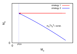
Figure 1: A sketch of the two approaches for chiral extrapolation to the physical point. Strategy 1 imposes the condition on the sum of the strange and light quark mass: $M_{\mathrm{s}}+\hat{M}=const.+O(M^{2})$, where $\hat{M}=(M_{\mathrm{u}}+M_{\mathrm{d}})/2$, while the second strategy keeps the strange quark mass $M_{\mathrm{s}}$ constant during the extrapolation.

From these we build pseudoscalars, pions with mass $m_{\mathrm{\pi}}$ from two quarks with ${\kappa}_{1}$ and ${\kappa}_{2}$. The kaons we build from $(\hat{\kappa},\kappa_{3})$. The physical point is defined by $m_{\mathrm{\pi,phys}}=134.8\mathrm{MeV}$ and $m_{\mathrm{K,phys}}=494.2\mathrm{MeV}$, the values in QCD with the electromagnetic interaction being switched off[9]. The two strategies differ in how $\kappa_{3}$ is chosen as a function of $\hat{\kappa}$.

In the following computations we have included the effect of the autocorrelations in the error analysis in a very conservative way. Namely, for the estimation of the error we take into account the tail of the autocorrelation function[8]. Thus, we are convinced that we have statistical errors fully under control. The examples of autocorrelation functions for $f_{\mathrm{\pi}}$ and $f_{\mathrm{K}}$ are shown in Figure 3. They are computed following the procedures detailed in [10].

3.1 SU(3) Chiral Perturbation Theory (Strategy 1)

In this approach we define the strange quark hopping parameter $\kappa_{3}$ through the dimensionless ratio

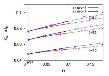
Figure 2: Chiral extrapolation of the kaon decay constant in lattice units. The values of $f_{\mathrm{K}}$ have been multiplied by $Z_{A}^{-1}$, but the error shown does not take the statistical error of the renormalization constant into account. The extrapolated results coming from both strategies agree at the physical point. They are obtained by applying the global fit for all three values of gauge couplings $\beta$, imposing a cut $\hat{y}_{\pi}<0.1$.

$$\frac{m_{\mathrm{K}}^{2}(\hat{\kappa},\kappa_{3})}{f_{\mathrm{K}}^{2}(\hat{\kappa},\kappa_{3})}=\frac{m_{\mathrm{K,phys}}^{2}}{f_{\mathrm{K,phys}}^{2}},$$ (1)

for each value $\hat{\kappa}$ and the gauge coupling ($\beta$), such that the l.h.s. of the equation remains equal to the constant $R=\frac{m_{\mathrm{K,phys}}^{2}}{f_{\mathrm{K,phys}}^{2}}$. Rather than a fixed strange quark mass, this corresponds to $M_{\mathrm{s}}+\hat{M}=const.$ to lowest order in the expansion in the quark masses and this is expected to give a flat chiral extrapolation for $f_{\mathrm{K}}$. The condition (1) determines a value of $\kappa_{3}=h(\hat{\kappa})$ as a function of the sea quark hopping parameter and it can be obtained by interpolation. After the dependence of $\kappa_{3}$ on $\hat{\kappa}$ is determined, it remains to extrapolate the decay constant $af_{\mathrm{K}}(\hat{\kappa},h(\hat{\kappa}))$ to the physical point, defined by the dimensionless ratio

$$\frac{m_{\mathrm{\pi}}^{2}(\hat{\kappa},h(\hat{\kappa}))}{f_{\mathrm{K}}^{2}(\hat{\kappa},h(\hat{\kappa}))}=\frac{m_{\mathrm{\pi,phys}}^{2}}{f_{\mathrm{K,phys}}^{2}}.$$ (2)

In the last step we use the prediction of this functional form coming from SU(3) ChPT[11]:

$${a}f_{\mathrm{K}}(\hat{\kappa},h(\hat{\kappa}))~{} = ~{}{a}f_{\mathrm{K,lat}}\big{[}1+\bar{L}_{\mathrm{K}}(\hat{y}_{\mathrm{\pi}},y_{\mathrm{K}})+({\alpha_{4}}-\frac{1}{4})(\hat{y}_{\mathrm{\pi}}-y_{\mathrm{\pi}})+O(y^{2})\big{]},$$ (3)

$$\bar{L}_{\mathrm{K}}(\hat{y}_{\mathrm{\pi}},y_{\mathrm{K}}) = -\frac{1}{2}\hat{y}_{\mathrm{\pi}}\log(\hat{y}_{\mathrm{\pi}})-\frac{1}{8}\hat{y}_{\mathrm{\pi}}\log(\frac{2y_{\mathrm{K}}}{\hat{y}_{\mathrm{\pi}}}-1)+\frac{1}{2}y_{\mathrm{\pi}}\log(y_{\mathrm{\pi}})+\frac{1}{8}y_{\mathrm{\pi}}\log(y_{\mathrm{\pi}}),$$ (4)

where ${a}f_{\mathrm{K,lat}}$ is the value of the decay constant in lattice units and the variables $y$ are defined as

$$\hat{y}_{\mathrm{\pi}}=\frac{m_{\mathrm{\pi}}^{2}(\hat{\kappa})}{8\pi^{2}f_{\mathrm{K}}^{2}(\hat{\kappa})}~{}~{}~{}~{}~{}~{}y_{\mathrm{K}}=\frac{m_{\mathrm{K,phys}}^{2}}{8\pi^{2}f_{\mathrm{K,phys}}^{2}}~{}~{}~{}~{}~{}~{}y_{\mathrm{\pi}}=\frac{m_{\mathrm{\pi,phys}}^{2}}{8\pi^{2}f_{\mathrm{K,phys}}^{2}}.$$ (5)

The described chiral extrapolation to the physical point is shown in Figure 2. Finally, the lattice spacings for each value of the gauge coupling can be obtained with

$$a=\frac{af_{\mathrm{K,lat}}}{f_{\mathrm{K,phys}}}$$ (6)

and its values, together with the errors of this determination, are shown in Table 2.

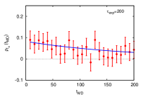
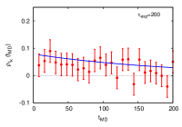
Figure 3: Autocorrelation functions of pion decay constant(left) and kaon decay constant(right). In the error computation the tail of the autocorrelation function is taken into account. Standard truncations of the integral lead to an error smaller by a factor 2 or more.

3.2 Heavy Meson Chiral Perturbation Theory (Strategy 2)

In this approach, we work at the fixed strange quark mass and perform a chiral extrapolation in the light quark mass ($\hat{M}$) using HMChPT [12]. Since we are working with Wilson fermions, one has to keep fixed the axial Ward identity (PCAC) mass of the strange quark. If we denote

$${m}_{{ij}}~{}=~{}\frac{1}{2}\frac{\langle\tilde{\partial_{0}}~{}A^{ij}_{0,\mathrm{I}}~{}{{P^{ji}}}\rangle}{\langle{P^{ij}}~{}{{P^{ji}}}\rangle},$$ (7)

with ${P^{ij}}=\bar{\psi_{i}}(x)\gamma_{5}{\psi_{j}}(x)$ and $A^{ij}_{0,\mathrm{I}}(x)=\bar{\psi_{i}}(x)\gamma_{0}\gamma_{5}{\psi_{j}}(x)+{a}~{}c_{\mathrm{A}}\tilde{\partial_{0}}{P^{ij}}(x)$ being pseudoscalar density and improved axial current, then the bare PCAC masses of the sea and the valence quark are defined by

$$m_{1}(\hat{\kappa})~{}=~{}m_{12}~{}~{}~{}~{}~{}~{}~{}m_{3}(\hat{\kappa},\kappa_{3})~{}=~{}m_{34}.$$ (8)

We first interpolate in $\kappa_{3}$ and determine functions $s(\hat{\kappa},\mu)$ such that the strange quark mass is kept fixed to $m_{3}(\hat{\kappa},s(\hat{\kappa},\mu))=\mu$. For fixed $\mu$ we then perform a HMChPT extrapolation to the chiral limit defined by $m_{\mathrm{\pi,phys}}^{2}/f_{\mathrm{K,phys}}^{2}$ [13, 14] using

$${a}~{}f_{\mathrm{K}}(\hat{\kappa},s(\hat{\kappa},\mu))~{} = ~{}P(\mu)\big{[}1-\frac{3}{8}[\hat{y}_{\mathrm{\pi}}\log(\hat{y}_{\mathrm{\pi}})-y_{\mathrm{\pi}}\log(y_{\mathrm{\pi}})]+{\alpha_{\mathrm{H}}}(\hat{y}_{\mathrm{\pi}}-y_{\mathrm{\pi}})+O(M^{2})\big{]}$$ (9)

$${a^{2}}m_{\mathrm{K}}^{2}(\hat{\kappa},s(\hat{\kappa},\mu))~{} = Q(\mu)\big{[}1+\alpha^{\prime}_{\mathrm{H}}(\hat{y}_{\mathrm{\pi}}-y_{\mathrm{\pi}})+O(M^{2})\big{]}.$$ (10)

In the end, the scale is obtained by interpolation in $\mu$ to the physical strange quark mass

$$a=\frac{P(\mu_{\mathrm{K}})}{f_{\mathrm{K}}}~{}~{}~{}\mathrm{at}~{}~{}~{}\frac{Q(\mu_{\mathrm{K}})}{P(\mu_{\mathrm{K}})^{2}}=\frac{m_{\mathrm{K,phys}}^{2}}{f_{\mathrm{K,phys}}^{2}}.$$ (11)

The values of the lattice spacings from this strategy are shown in Table 2. Comparing to the results of the first strategy, we find a very good agreement as demonstrated in Figure 2.

	Strategy 1			Strategy 2
$\beta$	5.2	5.3	5.5	5.2	5.3	5.5
$a[\mathrm{fm}]$	0.0750	0.0655	0.04847	0.0745	0.0649	0.04808
$\Delta_{\mathrm{stat.}}a$	0.0024	0.0010	0.00048	0.0025	0.0010	0.00047
$\Delta_{\mathrm{syst.}}a$	0.0013	0.0011	0.00079	0.0014	0.0012	0.00090

Table 2: Lattice spacings from the first strategy obtained by applying SU(3) ChPT(left) and from the second strategy, based on HMChPT(right). Estimation of the systematical errors is preliminary.

4 Determination of $\Lambda$ and $\overline{m}_{\mathrm{s}}$

In the $N_{\mathrm{f}}=2$ theory, low and high energy physics have been connected non-perturbatively by the ALPHA Collaboration, using an intermediate (Schrödinger functional) renormalization scheme[1, 2]. Here QCD is formulated in a finite box of spatial size $L$ and temporal extent $T$. The fields are subject to Dirichlet boundary conditions in time and periodic in space, where the former provide an infrared cutoff to the modes of quarks and gluons. This allows to perform simulations at zero quark mass and thus use the SF as a mass-independent renormalization scheme. We additionally specify that $T\equiv L$ and then the renormalization conditions are naturally imposed at the scale $\mu=1/L$.

To calibrate the overall energy scale, one fixes a large enough value of the coupling $\bar{g}^{2}(L_{\mathrm{max}})$ to be in the low-energy region and relates the associated distance, $L_{\mathrm{max}}$, to a non-perturbative, infinite-volume observable, in our case $f_{\mathrm{K}}$. The extrapolation of the combination $f_{\mathrm{K}}L_{\mathrm{max}}$ to the continuum limit is shown in Figure 4(left). It has been performed for both strategies of scale determination and the results agree within the errorbars. Combining the continuum result $(f_{\mathrm{K}}L_{\mathrm{max}})_{\mathrm{cont}}~{}=~{}0.318(14)(6)$ and the value of $({\Lambda}_{\mathrm{\overline{MS}}}L_{\mathrm{max}})$ from [2] we get the updated value of the $\mathrm{\overline{MS}}$ $\Lambda$-parameter in two flavor QCD:

$${\Lambda^{(2)}_{\mathrm{\overline{MS}}}}={\frac{1}{(f_{\mathrm{K}}L_{\mathrm{max}})}}{({\Lambda}_{\mathrm{\overline{MS}}}L_{\mathrm{max}})}f_{\mathrm{K}}=316(26)(17)\mathrm{MeV},$$ (12)

where the matching has been performed at the low energy scale $1/L_{\mathrm{max}}$, defined with $\bar{g}^{2}(L_{\mathrm{max}})=4.484$ and $f_{\mathrm{K}}$ is the experimental value of the kaon decay constant.

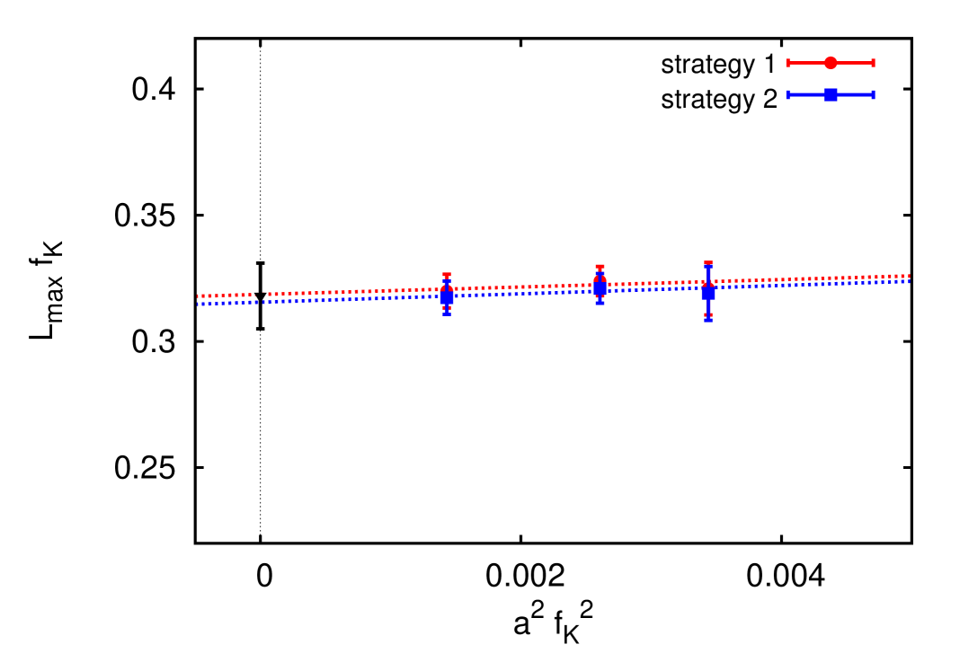
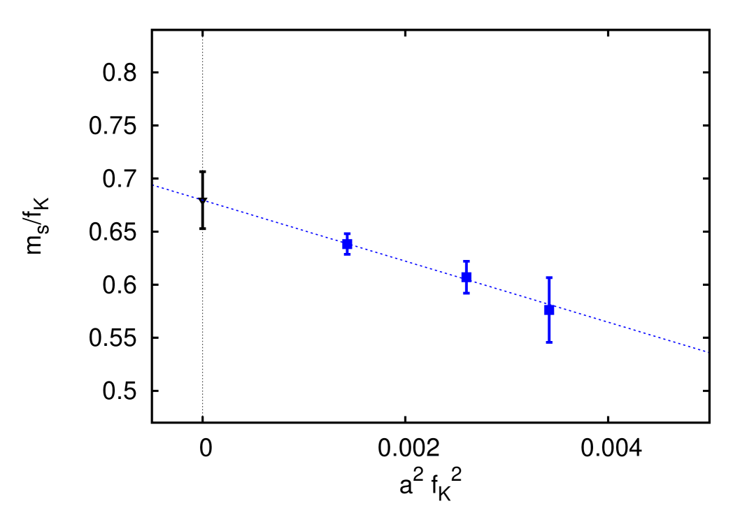
Figure 4: Chiral extrapolations of the product of lattice kaon decay constant $f_{\mathrm{K}}$ and matching scale $L_{\mathrm{max}}$, defined with $\bar{g}^{2}(L_{\mathrm{max}})=4.484$ (left) and bare strange quark mass in units of $f_{\mathrm{K}}$(right). The matching scale in the extrapolation of $m_{\mathrm{s}}$(right) is defined with $\bar{g}^{2}(\tilde{L}_{\mathrm{max}})=4.61$

Furthermore, we compute the strange quark mass. We base it on the PCAC mass $\mu_{\mathrm{K}}$ from the second strategy for chiral extrapolation (cf. Sect.3.2.). The $\mathrm{\overline{MS}}$ strange quark mass is given by (small corrections proportional to the quark masses in lattice units are also accounted for)

$$\overline{m}_{\mathrm{s}~{}\mathrm{\overline{MS}}}^{(2)}~{}(2\mathrm{GeV})~{}=\frac{M}{\overline{m}_{\mathrm{SF}}(\tilde{L}_{\mathrm{max}})}\,\frac{Z_{\mathrm{A}}\mu_{\mathrm{K}}}{Z_{\mathrm{P}}(\tilde{L}_{\mathrm{max}})f_{\mathrm{K}}}\,\frac{\overline{m}_{\mathrm{\overline{MS}}}(2\mathrm{GeV})}{M}\,f_{\mathrm{K}}=101.4(4.2)(2.5)\mathrm{MeV},$$ (13)

where the first factor is taken over from [1], and the new continuum extrapolation of the second factor is shown in the right panel of the Figure 4. Here, the matching scale is defined with $\bar{g}^{2}(\tilde{L}_{\mathrm{max}})=4.61$. The conversion factor to $\mathrm{\overline{MS}}$ scheme $\frac{\overline{m}_{\mathrm{\overline{MS}}}}{M}(\mu=2\mathrm{GeV})=0.7431$ is computed at 4-loop perturbation theory; all other factors are non-perturbative.

5 Summary and outlook

An important step missing in our previous work on non-perturbative renormalization of two flavor QCD has been performed. The scale is set from a physical quantity $f_{\mathrm{K}}$. Two strategies of chiral extrapolation are used and both give comparable results. Finally, we presented the non-perturbative computation of the $\Lambda$ parameter and the strange quark mass of two flavor QCD. The only perturbative input in the whole calculation is the 4-loop conversion factor from the RGI strange quark mass to $\mathrm{\overline{MS}}$ strange quark mass, which is required to make contact with wide spread conventions.

6 Acknowledgements

We thank O.Bär, P. Fritzsch, B. Leder, F. Knechtli, H. Simma and U.Wolff for useful and stimulating discussions. This work is supported by the German Science Foundation (DFG) under the grants GRK1504 ”Mass, spectrum, symmetry” and SFB/TR9-03. Simulations were performed at JUGENE and JUROPA supercomputers at Forschung Zentrum Jülich, HLRN in Berlin and Hannover and the PAX Clusters at DESY, Zeuthen.

References

- [1] M. Della Morte et al. [ ALPHA Collaboration ], Nucl. Phys. B729 (2005) 117-134. [hep-lat/0507035].
- [2] M. Della Morte et al. [ ALPHA Collaboration ], Nucl. Phys. B713 (2005) 378-406. [hep-lat/0411025].
- [3] M. Göckeler et al. [ QCDSF and UKQCD Collaborations ], Phys. Lett. B639 (2006) 307-311. [hep-ph/0409312].
- [4] B. Leder, F. Knechtli, PoS LAT2011 (2011) 315. [arXiv:1112.1246v2 [hep-lat]]
- [5] D. Pleiter [ QCDSF Collaboration ], PoS LAT2011 (2011) 235.
- [6] M. Lüscher, Comput. Phys. Commun. 165 (2005) 199-220. [hep-lat/0409106].
- [7] M. Marinkovic, S. Schaefer, PoS LATTICE2010 (2010) 031. [arXiv:1011.0911 [hep-lat]].
- [8] S. Schaefer et al. [ ALPHA Collaboration ], Nucl. Phys. B845 (2011) 93-119. [arXiv:1009.5228 [hep-lat]].
- [9] G. Colangelo, et al., Eur. Phys. J. C71 (2011) 1695. [arXiv:1011.4408 [hep-lat]].
- [10] U. Wolff, Comput. Phys. Commun. 156 (2004) 143153, [hep-lat/0306017].
- [11] S. R. Sharpe, Phys. Rev. D56 (1997) 7052-7058. [hep-lat/9707018].
- [12] T. Bhattacharya, R. Gupta, W. Lee, S. R. Sharpe, J. M. S. Wu, Phys. Rev. D73 (2006) 034504. [hep-lat/0511014].
- [13] A. Roessl, Nucl. Phys. B555 (1999) 507-539. [hep-ph/9904230].
- [14] C. Allton et al. [ RBC-UKQCD Collaboration ], Phys. Rev. D78 (2008) 114509. [arXiv:0804.0473 [hep-lat]].