Quantum phase transitions of ultra-cold Bose system in non-rectangular optical lattices

Abstract

In this paper, we investigate systematically the Mott-insulator-Superfluid quantum phase transitions for ultracold scalar bosons in triangular, hexagonal, as well as Kagomé optical lattices. With the help of field-theoretical effective potential, by treating the hopping term in Bose-Hubbard model as perturbation, we calculate the phase boundaries analytically for different integer filling factors. Our analytical results are in good agreement with recent numerical results.

I Introduction

The physics of dilute ultracold quantum gases in optical lattices has grown to one of the most fascinating fields over the last decade bloch-rmp2008 ; jaksch-zoller-ap ; lewenstein . In the case of bosons, the delicate balance between the atom-atom on-site interaction and the hopping amplitude leads to a quantum phase transition sachdev-qptbook between two distinct phases fisher ; zoller ; greiner . When the on-site interaction is small compared to the hopping amplitude, the ground state is superfluid, as the bosons are phase coherent and delocalized. In the opposite limit of the strong on-site repulsion, the ground state is a Mott-insulator, as every boson is trapped in one of the potential minima. Meanwhile, this clean defectless setup, which allows for precise control of its paramters, has opened up testing ground for quantum many-body physics, i.e. the so-called quantum simulation lewenstein .

While most experiments with ultracold atoms up to date have been performed in simple cubic lattices due to the ease of their experimental implementation petsas-pra1994 , recent work have explored ultra-cold atoms in non-standard optical lattices such as triangularsengstock-njp and hexagonal optical lattices sengstock-hexagonal , even the Kagomé optical lattices has also been recognized couple of months ago kagome-lattice . In fact, due to the complex of the lattice structure in these systems, novel and rich new phases will be exhibited. Hence, to determine the quantum phase diagrams analytically in these systems becomed a major problem and need to be investigated systematically.

Actually, there are two main analytical methods which can be used to determine the phase boundaries of Bose gases. One is the mean-field theory fisher , the other one is the so-called strong-coupling expansion freericks-1 . However, comparison with the Monte Carlo data capogrosso-1 shows that the mean-field theory underestimates the location of the phase boundary while the strong-coupling expansion goes in the opposite direction. More recently, an alternative analytical treatment based on the effective potential and Rayleigh-Schrödinger perturbation theory has been presented axel-09 , this novel method may, in principle, yields analytical results for phase boundaries at arbitrary dimension and lobe number in arbitrarily high order accuracy.

In this paper, with the help of this novel systematic approach, we are going to determine the Mott-Insulator-Superfluid (MI-SF) quantum phase boundaries of ultracold scalar Bose systems in triangular lattice, hexagonal lattice and Kagomé lattice analytically, and present the corresponding expressions of the phase boundaries. Comparing to numerical solutions, the relative deviation of our third-order analytical results is less than 10%.

II The model and the effective potential method

A system of spinless bosons trapped in a homogeneous optical lattice can be described by the simple yet nontrivial Bose-Hubbard Hamiltonian bloch-rmp2008 ; bloch which reads

$$H_{\mathrm{BH}}=-t\sum_{\langle i,j\rangle}\hat{a}_{i}^{\dagger}\hat{a}_{j}+\sum_{i}\frac{U}{2}\hat{n}_{i}(\hat{n}_{i}-1)-\mu\hat{n}_{i}$$ (1)

with $t$ being nearest neighbor hopping parameter while $U$ denoting the strength of on-site repulsion between two atoms, $\hat{n}_{i}=\hat{a}_{i}^{\dagger}\hat{a}_{i}$ are the corresponding particle number operator. $\mu$ is the chemical potential. When the depth of the optical lattice wells is increased, the hopping parameter $t$ decreases exponentially while $U$ increases linearly zwerger-1 .

In order to investigate the superfluid-Mott insulator phase transition systematically and to determine the corresponding phase boundary analytically in a more accurate way, we are going to tackle this issue via field theory, or namely, the effective potential method axel-09 . To this end, we add for the moment additional source terms with strength $J$ and $J^{*}$ into the Bose-Hubbard Hamiltonian as following

$$\hat{H}_{BH}(J^{\ast},J)=-t\sum_{\langle i,j\rangle}\hat{a}_{i}^{\dagger}\hat{a}_{j}+\sum_{i}(J^{\ast}\hat{a}_{i}+J\hat{a}_{i}^{\dagger})+\hat{H}_{0},$$ (2)

and treat the hopping term and external source terms as perturbations. Here

$$\hat{H}_{0}=\sum_{i}\frac{U}{2}\hat{n}_{i}(\hat{n}_{i}-1)-\mu\hat{n}_{i}$$ (3)

is the unperturbed part of the Hamiltonian.

It is quite straightforward that the grand-canonical free energy can be presented as power series of both the hopping parameter $t$ and the source $J,J^{\ast}$ via Taylor’s expansions. Since the unperturbed ground states are Mott states with the same occupation number on each site, i.e. the unperturbed state is local, $J$ and $J^{*}$ can only appear in pair in the expansion. After regrouping the terms in the free energy with respect of $J$ and $J^{*}$, the free energy reads

$$F(J^{\ast},\,J,\,t)=N_{s}\left(\,F_{0}(t)+\sum_{p=1}^{\infty}c_{2p}(t)\mid J\mid^{2p}\,\right)\,,$$ (4)

with the expansion coefficients

$$c_{2p}(t)=\sum_{n=0}^{\infty}(-t)^{n}\,\alpha_{2p}^{(n)}$$ (5)

being power series of hopping parameter $t$, $N_{s}$ is the total number of lattice sites.

The superfluid order parameter $\psi=\langle\hat{a}_{i}\rangle$ and its complex conjugate can then be calculated by H.kleinert 09 ; J.Zinn-Justin 09

$$\psi=\frac{1}{N_{s}}\frac{\partial F(J^{\ast},\,J,\,t)}{\partial J^{\ast}},\quad\psi^{\ast}=\frac{1}{N_{s}}\frac{\partial F(J^{\ast},\,J,\,t)}{\partial J}.$$ (6)

With the help of the above formula, a Legendre transformation of the grand-canonical free energy can thus be conducted, leading to the effective potential as follows:

$$\Gamma{(\psi,\,\psi^{\ast})}=\frac{F}{N_{s}}-\psi^{\ast}J-\psi J^{\ast}.$$ (7)

Substituting Eq.(4) into Eq.(6), the relation between the order parameter and the external source strength is obtained and can then be used to eliminate $J$ and $J^{*}$ in Eq. (7), giving

$$\Gamma=F_{0}(t)-\frac{1}{c_{2}(t)}\mid\psi\mid^{2}+\,\frac{c_{4}(t)}{c_{2}(t)^{4}}\mid\psi\mid^{4}\,+\cdots.$$ (8)

Apparently the effective potential takes exactly the form of $\phi^{4}$ theory. Indeed, from Eq.(7), it is immediately recognized that the external sources can be expressed as

$$\frac{\partial\Gamma(\psi,\,\psi^{\ast})}{\partial\psi^{\ast}}=-J,\qquad\frac{\partial\Gamma(\psi,\,\psi^{\ast})}{\partial\psi}=-J^{\ast}.$$ (9)

Recalling that the original physical system what we are interested in is a system with vanishing external sources, this equation shows that the physical states correspond to the saddle points of the effective potential. As is known, in $\phi^{4}$ theory the phase transitions is marked by the sign change of the coefficient of the quadratic term, indicating that for our system the phase boundary can be found by letting $\frac{1}{c_{2}(t)}=0$, the solution of this equation will provide us the critical value of $t$.

Actually, as shown in Eq.(5), $c_{2}(t)$ is a power series of $t$, thus the radius of convergence of $c_{2}(t)$ will reveal the location of the phase boundary. Accordingly, the $n$-th order approximation of the phase boundary is given by

$$t_{c}^{(n)}=-\frac{\alpha_{2}^{(n-1)}}{\alpha_{2}^{(n)}}.$$ (10)

This equation shows that, in principle, the phase boundary of the Bose-Hubbard system can be calculated out analytically with arbitrarily high accuracy via the field theory method or effective potential method. It should be pointed out that in the pioneer work axel-09 in this field, the expression of the phase boundary is different from what we got above. The reason is that in that work, $\frac{1}{c_{2}(t)}$ was inconveniently expanded to a power series of $t$. However, this inconvenience would not affect the credit of that elegant work.

III Arrow-line diagram representation

From the above discussion, we have translated the problem of finding the phase boundary to the problem of calculating the coefficient $\alpha_{2}^{(n)}$. These quantities can be calculated via linked cluster expansion metzner and Rayleigh-Schrödinger perturbation theory, or namely the Kato’s formulation kato .

Since the unperturbed state corresponding to the unperturbed Hamiltonian $H_{0}$ is Mott state with all lattice sites occupied by the same number of bosons, thus, according to Eq. (2), in the free energy $F(J^{*},J,t)$ (4), between the bra and ket of the unperturbed ground state, every non-zero contribution to $\alpha_{2}^{(n)}$ includes exactly one creation operator at $i$-th site (associated with $J_{i}$) and one annihilation operator at $j$-th site (associated with $J^{*}_{i}$) as well as $n$ nearest neighboring hopping processes (associated with $t$) connecting $i$ and $j$ sites via other neighboring lattice sites. $i$-th and $j$-th sites could be the same.

Table 1: Diagrammatic expressions of $\alpha_{2}^{(n)}$ for triangular lattice, hexagonal lattice and Kagomé lattice

	triangular lattice	hexagonal lattice	kagome lattice
$\alpha_{2}^{(0)}$
$\alpha_{2}^{(1)}$	$6\includegraphics[width=56.9055pt]{2.eps}$	$3\includegraphics[width=56.9055pt]{2.eps}$	$4\includegraphics[width=56.9055pt]{2.eps}$
$\alpha_{2}^{(2)}$	$6\includegraphics[width=56.9055pt]{3.eps}+30\includegraphics[width=56.9055pt]{4.eps}$	$3\includegraphics[width=56.9055pt]{3.eps}+6\includegraphics[width=56.9055pt]{4.eps}$	$4\includegraphics[width=56.9055pt]{3.eps}+12\includegraphics[width=56.9055pt]{4.eps}$
	$138\includegraphics[width=85.35826pt]{5.eps}$	$12\includegraphics[width=85.35826pt]{5.eps}$	$32\includegraphics[width=85.35826pt]{5.eps}$
$\alpha_{2}^{(3)}$	$+30\includegraphics[width=56.9055pt]{7.eps}+30\includegraphics[width=56.9055pt]{6.eps}$	$+6\includegraphics[width=56.9055pt]{7.eps}+6\includegraphics[width=56.9055pt]{6.eps}$	$+12\includegraphics[width=56.9055pt]{7.eps}+12\includegraphics[width=56.9055pt]{6.eps}$
	$+6\raisebox{-5.69046pt}{\includegraphics[width=56.9055pt]{8.eps}}+12\includegraphics[width=42.67912pt]{9.eps}$	$+3\raisebox{-5.69046pt}{\includegraphics[width=56.9055pt]{8.eps}}$	$+4\raisebox{-5.69046pt}{\includegraphics[width=56.9055pt]{8.eps}}+4\includegraphics[width=42.67912pt]{9.eps}$

When denoting a creation operator on a site by an arrow line pointing in this site and an annihilation operator by an arrow line pointing out of this site, each contribution of $\alpha_{2}^{(n)}$ can be sketched as an arrow-line diagram composed of $n$ oriented internal lines connecting the vertices and two external arrow lines, the vertices in the diagram correspond to respective lattice sites, oriented internal lines stand for the hopping process between sites, the two external arrow lines are directed into and out of a lattice site, respectively, representing creation and annihilation operators associated with the external sources. Each vertex in a diagram must has equal number of pointing-in lines and pointing-out lines. Actually, the diagrams are embedded in the lattices and, therefore, their topologies are determined by the topologies of underlying lattices. Table 1 presents all diagrams as well as the associated prefactors for the first four orders of $\alpha_{2}^{(n)}$ in triangular, hexagonal, and Kagomé lattices.

In order to determine the MI-SF quantum phase transitions of scalar Bose system in these non-rectangular lattices, the corresponding $\alpha_{2}^{(n)}$ in Table I need to be calculated explicitly, namely, these arrow-line diagrams should be translated to proper perturbation formulae.

IV Line-dot diagrams of perturbation calculation

Actually, perturbation calculation can be endowed with a line-dot diagrammatic representation axel-09 which can be used to simplify the calculation of above mentioned $\alpha_{2}^{(n)}$ diagrams. In order to make the paper self-contained, let us here give a brief review of this graphic representation of the perturbation theory, for detail technique please refer to Ref.axel-09 .

Suppose the total Hamiltonian is $H=H_{0}+gV$ in which $V$ is a perturbation with small parameter $g$. In general, the eigenenergy of the Hamiltonian $H$ is $E_{n}=\sum_{i=0}^{\infty}g^{i}E_{n}^{\left(i\right)}$ , where

$$E_{n}^{\left(i\right)}=\left\langle\Psi_{n}^{\left(0\right)}\right|V\left|\Psi_{n}^{\left(i-1\right)}\right\rangle$$ (11)

with

$$\left|\Psi_{n}^{\left(i\right)}\right\rangle=\sum_{m\neq n}\left|\Psi_{m}^{\left(0\right)}\right\rangle\frac{\left\langle\Psi_{m}^{\left(0\right)}\right|V\left|\Psi_{n}^{\left(i-1\right)}\right\rangle}{E_{n}^{\left(0\right)}-E_{m}^{\left(0\right)}}-\sum_{j=1}^{i}E_{n}^{\left(j\right)}\sum_{m\neq n}\left|\Psi_{m}^{\left(0\right)}\right\rangle\frac{\left\langle\Psi_{m}^{\left(0\right)}|\Psi_{n}^{\left(i-j\right)}\right\rangle}{E_{n}^{\left(0\right)}-E_{m}^{\left(0\right)}},$$

where $\left|\Psi_{n}^{\left(0\right)}\right\rangle$ is the $n$-th eigenstate of unperturbed part $H_{0}$ while $E_{n}^{\left(0\right)}$ is the corresponding eigenenergy. These complicated forumulae have a simple brief graphic representation. The detailed expression of $E_{n}^{\left(i\right)}$ in Eq.(11) can be represented as a combination of dots and lines by making use of the following rules: (1) each dot represents an interaction $V$; (2) $p$ internal lines connecting two adjacent dots stand for $\sum_{m\neq n}\frac{1}{\left(E_{n}^{\left(0\right)}-E_{m}^{\left(0\right)}\right)^{p}}\left|\Psi_{m}^{\left(0\right)}\right\rangle\left\langle\Psi_{m}^{\left(0\right)}\right|$; (3) $\left\langle\Psi_{n}^{\left(0\right)}\right|$ and $\left|\Psi_{n}^{\left(0\right)}\right\rangle$ can only be denoted by the left-external and right-external lines, respectively. From the third rule, it is easy to recognize that in the diagrammatic representation of $E_{n}^{\left(i\right)}$ there are some graphs which consist of disconnected parts, the sign in front of this type of graphs is $\left(-1\right)^{s-1}$, where $s$ is the number of the disconnected parts in this graph.

To illustrate these rules more clearly, as an example, let us concentrate on $E_{n}^{\left(3\right)}$. From Eq. (11), it reads

$$E_{n}^{\left(3\right)} =\sum_{m_{1}\neq n}\sum_{m_{2}\neq n}\left\langle\Psi_{n}^{\left(0\right)}\right|V\frac{\left|\Psi_{m_{2}}^{\left(0\right)}\right\rangle\left\langle\Psi_{m_{2}}^{\left(0\right)}\right|}{E_{n}^{\left(0\right)}-E_{m_{2}}^{\left(0\right)}}V\frac{\left|\Psi_{m_{1}}^{\left(0\right)}\right\rangle\left\langle\Psi_{m_{1}}^{\left(0\right)}\right|}{E_{n}^{\left(0\right)}-E_{m_{1}}^{\left(0\right)}}V\left|\Psi_{n}^{\left(0\right)}\right\rangle$$

$$-\sum_{m\neq n}\left\langle\Psi_{n}^{\left(0\right)}\right|V\left|\Psi_{n}^{\left(0\right)}\right\rangle\left\langle\Psi_{n}^{\left(0\right)}\right|V\frac{\left|\Psi_{m}^{\left(0\right)}\right\rangle\left\langle\Psi_{m}^{\left(0\right)}\right|}{\left(E_{n}^{\left(0\right)}-E_{m}^{\left(0\right)}\right)^{2}}V\left|\Psi_{n}^{\left(0\right)}\right\rangle,$$

then, by utilizing the rules mentioned above, we have

$$E_{n}^{\left(3\right)}=\;\;\includegraphics[width=56.9055pt]{d2.eps}-\raisebox{-8.5359pt}{\includegraphics[width=42.67912pt]{d3.eps}}.$$ (12)

This procedure can be extended to cases with several perturbation terms axel-09 . However, in those cases, dots may represents different perturbations and should be labelled by different numbers, hence the line-dot diagrams mentioned above are now extended to sums of all possible permutations with respective topology. All the diagrams must be read from right to left to present correct formula.

V Quantum Phase diagrams of Bose systems in non-rectangular optical lattices

With this line-dot diagrammatic representation of perturbation theory in hand, we now turn to our problem to see how the arrow diagrams included in $\alpha_{2}^{\left(n\right)}$ can be translated into the above mentioned line-dot diagrams.

As is known, each $\alpha_{2}^{\left(n\right)}$ consists of exactly one creation operator (associated with $J$), one annihilation operator (associated with $J^{*}$), and $n$ hopping operators (associated with $t^{n}$). Moreover, since the unperturbed ground state is local states, thus all these terms should be treated as different perturbations, i.e., each arrow in the arrow diagram of $\alpha_{2}^{\left(n\right)}$ corresponds to a dot in the respective line-dot diagram. Then with these dots, for each arrow-line diagram we draw all possible topologically different line-dot diagrams. The sum of these diagrams gives the corresponding result. To illustrate this more clearly, let us take as an example. This arrow diagram is a part of $\alpha_{2}^{\left(3\right)}$ in triangular lattice and Kagomé lattice. As discussed above, we label the five arrow lines explicitly as

(13)

These five processes correspond to five distinguishable points in line-dot diagrams. According to the translation rules discussed above, this arrow diagram can be reformulated in terms of line-dot diagrams as

$$= \includegraphics[width=56.9055pt]{d7.eps}\;-\;\raisebox{-5.69046pt}{\includegraphics[width=56.9055pt]{d4.eps}}\;-\;\raisebox{-5.69046pt}{\includegraphics[width=56.9055pt]{d5.eps}}\;-\;\raisebox{-5.69046pt}{\includegraphics[width=56.9055pt]{d6.eps}}.$$ (14)

Here, we should keep in mind that all these unnumbered line-dot diagram in the equation stand for the sum of all possible permutations. According to the line-dot diagram rule, all these diagrams can be calculated. Since here we are only concentrated on the properties of ground state, the calculation is relative straightforward.

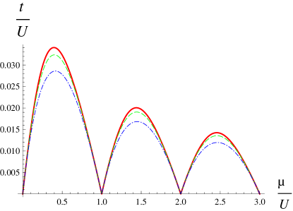
Figure 1: (color online) The phase boundaries of MI-SF quantum phase transition of Bose system in a triangle lattice at $T=0$. The red solid line is the third-order calculation, the green dashed line is the second-order result, while the blue dot dashed line is the first-order (mean-field) result.

By making use of the technique mentioned above, after a laborious yet straightforward calculation, the third order approximation of the phase boundaries in $t/U$-$\mu/U$ plane for scalar bosons in a triangular lattice with different integer filling factors are given by

$$t_{3} = -\frac{3(-3+\tilde{\mu})(-1+\tilde{\mu})\tilde{\mu}(-3-5\tilde{\mu}-7\tilde{\mu}^{2}-4\tilde{\mu}^{3}+3\tilde{\mu}^{4})U}{2(81+108\tilde{\mu}+135\tilde{\mu}^{2}+438\tilde{\mu}^{3}+164\tilde{\mu}^{4}-580\tilde{\mu}^{5}+266\tilde{\mu}^{6}-36\tilde{\mu}^{7})},\ \ \ \mathrm{for\ \ }n=1$$

$$t_{3} = \Big{[}(-4+\tilde{\mu})(-2+\tilde{\mu})(-1+\tilde{\mu})(1+\tilde{\mu})(12-129\tilde{\mu}+119\tilde{\mu}^{2}-37\tilde{\mu}^{3}$$

$$-20\tilde{\mu}^{4}+7\tilde{\mu}^{5})U\Big{]}\Big{/}\Big{[}2(-3056+13152\tilde{\mu}-23587\tilde{\mu}^{2}+7926\tilde{\mu}^{3}$$

$$+13446\tilde{\mu}^{4}-11688\tilde{\mu}^{5}+806\tilde{\mu}^{6}+1836\tilde{\mu}^{7}-623\tilde{\mu}^{8}+60\tilde{\mu}^{9})\Big{]},\ \ \mathrm{for\ \ }n=2$$

$$t_{3} = \Big{[}(-5+\tilde{\mu})(-3+\tilde{\mu})(-2+\tilde{\mu})\tilde{\mu}(1080-1781\tilde{\mu}+776\tilde{\mu}^{2}+14\tilde{\mu}^{3}$$ (15)

$$-82\tilde{\mu}^{4}+13\tilde{\mu}^{5})U\Big{]}\Big{/}\Big{[}2(-129600-72360\tilde{\mu}+707001\tilde{\mu}^{2}-859788\tilde{\mu}^{3}$$

$$+389390\tilde{\mu}^{4}-13498\tilde{\mu}^{5}-51903\tilde{\mu}^{6}+19658\tilde{\mu}^{7}-2980\tilde{\mu}^{8}+168\tilde{\mu}^{9})\Big{]},\ \ \mathrm{for\ \ }n=3$$

where $\tilde{\mu}=\mu/U$. These analytical results are shown in Fig. 1 together with the results for first order and second order calculation.

Our third-order analytical result shows that the tip of the $n=1$ Mott lobe phase boundary is located at $t_{c}/U=0.03406$, it has relative deviation of 9.7% from the systematic strong coupling expansion result elstner-monien and 9.4% from recent numerical result Nikalas Teichmann1 .

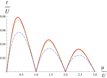
Figure 2: (color online) The phase boundaries of MI-SF quantum phase transition of Bose system in a hexagonal lattice at $T=0$. The red solid line is the third-order calculation, the green dashed line is the second-order result, while the blue dot dashed line is the first-order (mean-field) result.

The phase diagram of hexagonal lattice in $t/U$-$\mu/U$ plane has also been calculated out analytically via the same method, and the results are presented in Fig. 2. The tip of the first Mott lobe phase boundary of hexagonal system is located at $t_{c}/U=0.0787$, about 8.8% relatively deviating from the numerical result Nikalas Teichmann1 .

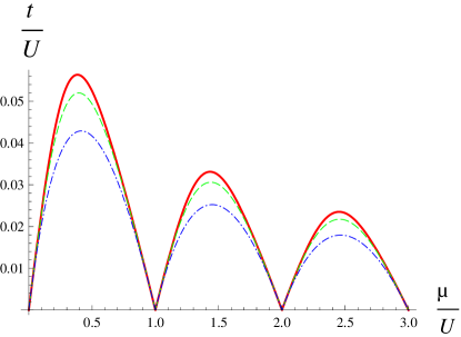
Figure 3: (color online) The phase diagram of MI-SF quantum phase transition of Bose system in a Kagomé lattice at $T=0$. The red solid line is the third-order calculation, the green dashed line is the second-order result, while the blue dot dashed line is the first-order (mean-field) result.

Kagomé-lattice many-body systems, due to their novelty, have attracted much attention in condensed matter research in recent decade. Naturally, it is worthy to spend more effort on quantum simulating them via ultra-cold atoms in optical Kagomé lattices. Fortunately, in recent days, this lattice has been realized in experiment kagome-lattice . Here, by making use the field-theory method, we also calculate the quantum phase diagram of scalar bosons in optical Kagomé lattice, the corresponding analytical expressions of the phase boundaries for different Mott lobes are

$$t_{c}^{(3)} = -\frac{(-3+\tilde{\mu})(-1+\tilde{\mu})\tilde{\mu}(-6-7\tilde{\mu}-15\tilde{\mu}^{2}-12\tilde{\mu}^{3}+8\tilde{\mu}^{4})U}{72+24\tilde{\mu}+113\tilde{\mu}^{2}+482\tilde{\mu}^{3}+203\tilde{\mu}^{4}-620\tilde{\mu}^{5}+274\tilde{\mu}^{6}-36\tilde{\mu}^{7}}\;\;\;\;{\rm for}\;\;n=1,$$ (16)

$$t_{c}^{(3)} = \Big{[}(-4+\tilde{\mu})(-2+\tilde{\mu})(-1+\tilde{\mu})(1+\tilde{\mu})(40-372\tilde{\mu}+377\tilde{\mu}^{2}$$ (17)

$$-101\tilde{\mu}^{3}-60\tilde{\mu}^{4}+20\tilde{\mu}^{5})\Big{]}U\Big{/}\Big{(}-10208+39280\tilde{\mu}-69668\tilde{\mu}^{2}+24200\tilde{\mu}^{3}$$

$$+41171\tilde{\mu}^{4}-35302\tilde{\mu}^{5}+1855\tilde{\mu}^{6}+5788\tilde{\mu}^{7}-1904\tilde{\mu}^{8}+180\tilde{\mu}^{9}\Big{)}\;\;\;\;{\rm for}\;\;n=2,$$

and

$$t_{c}^{(3)} = \Big{[}(-5+\tilde{\mu})(-3+\tilde{\mu})(-2+\tilde{\mu})\tilde{\mu}(1620-2669\tilde{\mu}+1171\tilde{\mu}^{2}+27\tilde{\mu}^{3}$$ (18)

$$-122\tilde{\mu}^{4}+19\tilde{\mu}^{5})\Big{]}U\Big{/}\Big{(}-194400-100440\tilde{\mu}+1027124\tilde{\mu}^{2}-1245918\tilde{\mu}^{3}$$

$$+551310\tilde{\mu}^{4}-4016\tilde{\mu}^{5}-82749\tilde{\mu}^{6}+30264\tilde{\mu}^{7}-4519\tilde{\mu}^{8}+252\tilde{\mu}^{9}\Big{)}\;\;\;\;{\rm for}\;\;n=3$$

respectively, where $\tilde{\mu}=\mu/U$.

VI Summary

In summary, with the help of effective potential theory, by treating the hopping term in Bose-Hubbard model and external sources as perturbations, and by conducting the linked cluster perturbation calculation, we investigate systematically the Mott-insulator-Superfluid quantum phase transitions for ultracold scalar bosons in triangular and hexagonal lattices, the corresponding analytical expressions of phase boundaries in these systems and corresponding phase diagrams have been presented. By comparing to recent numerical solutions, we have found that the relative deviation of our third-order analytical results is less than 10%.

Stimulated by the recent experimental result kagome-lattice in which the Kagomé optical lattice was realized first time, we have also calculated the MI-SF phase boundary for the scalar Bose system in optical Kagomé lattice. Our result may serve as a reference object for further studies. Meanwhile, as is known, in the non-rectangular lattice systems, due to the nontrivial lattice structures, novel and rich new phases will be exhibited, especially in systems in triangular lattice and in Kagomé lattice, since in these systems the geometrical frustration is possible under some specific circumstance. Our result presented in this paper may act as a starting point for further investigation in this direction.

References

- (1) I. Bloch, J. Dalibard, and W. Zwerger, Rev. Mod. Phys. 80, 885 (2008)
- (2) D. Jaksch and P. Zoller, Ann. Phys. 315, 52 (2005)
- (3) M. Lewenstein, A. Sanpera, V. Ahufinger, B. Damski, A. Sen De, and Ujjwal Sen, Adv. Phys. 56, 243 (2007)
- (4) S. Sachdev, Quantum Phase Transitions ( Cambridge University Press, Cambridge, U.K., 1999)
- (5) M.P.A. Fisher, P.B. Weichman, G. Grinstein, and D.S. Fisher, Phys. Rev. B 40, 546 (1989)
- (6) D. Jaksch, C. Bruder, J.I. Cirac, C.W. Gardiner, and P. Zoller, Phys. Rev. Lett. 81, 3108 (1998)
- (7) M. Greiner, O. Mandel, T. Esslinger, T.W. Hänsch, and I. Bloch, Nature 415, 39 (2002)
- (8) K. I. Petsas, A. B. Coates, and G. Grynberg, Phys. Rev. A 50, 5173 (1994)
- (9) C. Becker, P. Soltan-Panahi, J. Kronjäger, S. Dörscher, K. Bongs, K. Sengstock, New J. Phys. 12, 065025 (2010)
- (10) P. Soltan-Panahi, J. Struck, P. Hauke, A. Bick, W. Plenkers, G. Meineke, C. Becker, P. Windpassinger, M. Lewenstein, and K. Sengstock, Nature Physics 7, 434 (2011)
- (11) G.-B. Jo, J. Guzman, C.K. Thomas, P. Hosur, A. Vishwanath, and D.M. Stamper-Kurn, arXiv:1109.1591 (2011)
- (12) J.K. Freericks, and H. Monien, Phys. Rev. B 53, 2691 (1996)
- (13) B. Capogrosso-Sansone, N.V. Prokof’ev, and B.V. Svistunov, Phys. Rev. B 75, 134302 (2007)
- (14) F. E. A. dos Santos and A. Pelster, Phy. Rew.A 79 013614 (2009)
- (15) I. Bloch, Nature 453, 1016 (2008)
- (16) W. zwerger, J. Opt. B: Quantum Semiclassical Opt. 5, S9 (2003)
- (17) H. Kleinert and V.Schulte-Frohlinde, Critical Properties of -Theories (World Scientific, Singapore, 2001).
- (18) J.Zinn-Justin,Quantum Field Theory and Critical Phenomena(Oxford University Press, New York, 2004).
- (19) W. Metzner, Physical Review B 43, 8549 (1991)
- (20) T. Kato, Prog. Theor. Phys. 4, 514 (1949)
- (21) N. Elstner and H. Monien, Phys. Rev. B 59, 12184 (1999)
- (22) N. Teichmann,D. Hinrichs, and M. Holthaus, EPL 91, 10004 (2010).