Abstract

In this paper we study canonical $\gamma$-structures, a class of RNA pseudoknot structures that plays a key role in the context of polynomial time folding of RNA pseudoknot structures. A $\gamma$-structure is composed by specific building blocks, that have topological genus less than or equal to $\gamma$, where composition means concatenation and nesting of such blocks. Our main result is the derivation of the generating function of $\gamma$-structures via symbolic enumeration using so called irreducible shadows. We furthermore recursively compute the generating polynomials of irreducible shadows of genus $\leq\gamma$. $\gamma$-structures are constructed via $\gamma$-matchings. For $1\leq\gamma\leq 10$, we compute Puiseux-expansions at the unique, dominant singularities, allowing us to derive simple asymptotic formulas for the number of $\gamma$-structures.

Keywords: Generating function, Shape, Irreducible shadow, $\gamma$-structure.

1. Introduction and background

An RNA sequence is a linear, oriented sequence of the nucleotides (bases) A,U,G,C. These sequences “fold” by establishing bonds between pairs of nucleotides. These bonds cannot form arbitrarily, a nucleotide can at most establish one bond and the global conformation of an RNA molecule is determined by topological constraints encoded at the level of secondary structure, i.e., by the mutual arrangements of the base pairs Bailor et al. (2010).

Secondary structures can be interpreted as (partial) matchings in a graph of permissible base pairs Tabaska et al. (1998). When represented as a diagram, i.e. as a graph whose vertices are drawn on a horizontal line with arcs in the upper halfplane on refers to a secondary structure with crossing arcs as a pseudoknot structure.

Folded configurations exhibit the stacking of adjacent base pairs and specific minimum arc-length conditions Smith and Waterman (1978), where a stack is a sequence of parallel arcs $((i,j),(i+1,j-1),\dots,(i+\tau,j-\tau))$.

The topological classification of RNA structures Bon et al. (2008); Andersen et al. (2012b) has recently been translated into an efficient folding algorithm Reidys et al. (2011). This algorithm a priori folds into a novel class of pseudoknot structures, the $\gamma$-structures. $\gamma$-structures differ from pseudoknotted RNA structures of fixed topological genus of an associated fatgraph or double line graph Orland and Zee (2002) and Bon et al. (2008), since they have arbitrarily high genus. They are composed by irreducible subdiagrams whose individual genus is bounded by $\gamma$ and contain no bonds of length one ($1$-arcs), see Section 2 for details.

In Nebel and Weinberg (2011) Nebel and Weinberg study a plethora of RNA structures. The authors study asymptotic expansions for $\gamma=1$ and find that in the limit of large $n$ there are $j_{1}\,n^{-\frac{3}{2}}(\varrho_{1,1}^{-1})^{n}$, $1$-structures, where $\varrho_{1,1}^{-1}=3.8782$ and $j_{1}$ is some positive constant.

In this paper we study canonical $\gamma$-structures, i.e. partial matchings composed by irreducible motifs of genus $\leq\gamma$, without isolated arcs and $1$-arcs. These motifs are called irreducible shadows. We first establish a functional relationship between the generating function of $\gamma$-matchings and that of irreducible shadows. Via this relation, we identify a polynomial $P_{\gamma}(u,X)$, whose unique solution equals the generating function of $\gamma$-matchings. We then derive a recurrence of the generating function of irreducible shadows using Harer-Zagier recurrence Harer and Zagier (1986). The generating function of $\gamma$-matchings is then expanded at its unique dominant singularity as a Puiseux-series. This implies, by means of transfer theorems Flajolet and Sedgewick (2009), simple asymptotic formulas for the numbers of $\gamma$-matchings.

$\gamma$-matchings are the stepping stone to derive via Lemma 3 the further refined, bivariate generating function of $\gamma$-shapes, i.e. $\gamma$-matchings containing only stacks composed by a single arc. This generating function keeps additionally track of the $1$-arcs, that are vital for the later inflation into $\gamma$-structures. We then compute the generating function of $\tau$-canonical $\gamma$-structures inflating $\gamma$-shapes by means of symbolic enumeration.

2. Some basic facts

2.1. $\gamma$-diagrams

A diagram is a labeled graph over the vertex set $[n]=\{1,\dots,n\}$ in which each vertex has degree $\leq 3$, represented by drawing its vertices in a horizontal line. The backbone of a diagram is the sequence of consecutive integers $(1,\dots,n)$ together with the edges $\{\{i,i+1\}\mid 1\leq i\leq n-1\}$. The arcs of a diagram, $(i,j)$, where $i<j$, are drawn in the upper half-plane. We shall distinguish the backbone edge $\{i,i+1\}$ from the arc $(i,i+1)$, which we refer to as a $1$-arc.

A stack of length $\tau$ is a maximal sequence of “parallel” arcs,

$$((i,j),(i+1,j-1),\dots,(i+\tau,j-\tau)).$$

A stack of length $\geq\tau$ is called a $\tau$-canonical stack, i.e. a stack of length zero is an isolated arc. The particular arc $(1,n)$ is called a rainbow and an arc is called maximal if it is maximal with respect to the partial order $(i,j)\leq(i^{\prime},j^{\prime})$ iff $i^{\prime}\leq i\;\wedge j\leq j^{\prime}$, see Fig. 1.

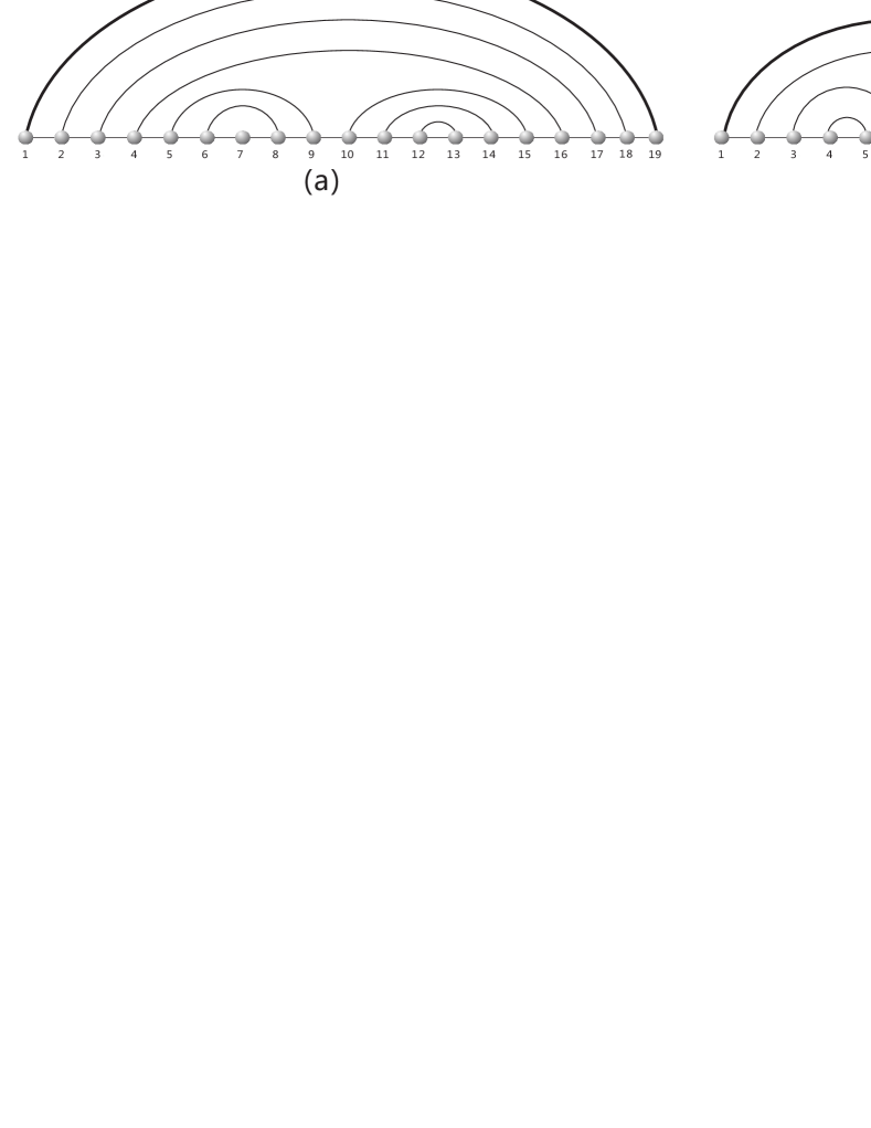
Fig. 1. $(a)$ a diagram containing a rainbow (bold), three stacks $((5,9),(6,8))$, $((10,15),(11,14),(12,13))$, and $((1,19),(2,18),(3,17),(4,16))$. $(b)$ the maximal arcs of a diagram displayed in (bold).

A stack of length $\tau$, $((i,j),(i+1,j-1),\dots,(i+\tau,j-\tau))$ induces a sequence of pairs $(([i,i+1],[j,j-1]),([i+1,i+2],[j-1,j-2])\dots([i+\tau-1,i+\tau],[j-\tau,j-\tau+1]))$. We call any of these $2\tau$ intervals a $P$-interval. The interval $[i+\tau,j-\tau]$ is called a $\sigma$-interval, see Fig. 2.

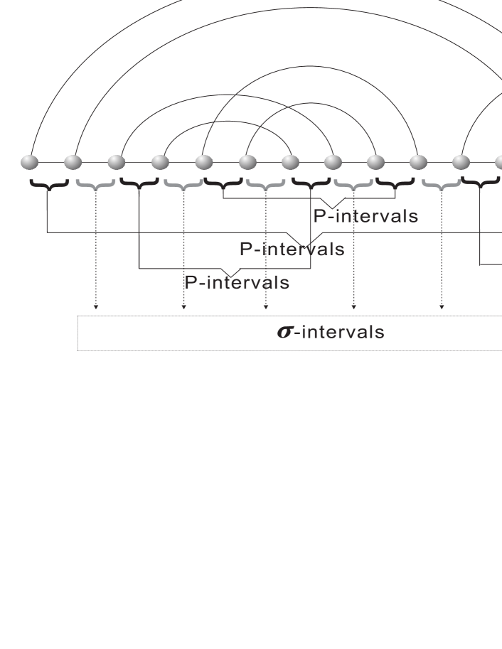
Fig. 2. $\sigma$- and $P$-intervals.

We shall consider diagrams as fatgraphs, $\mathbb{G}$, that is graphs $G$ together with a collection of cyclic orderings, called fattenings, one such ordering on the half-edges incident on each vertex. Each fatgraph $\mathbb{G}$ determines an oriented surface $F(\mathbb{G})$ Loebl and Moffatt (2008); Penner et al. (2010) which is connected if $G$ is and has some associated genus $g(G)\geq 0$ and number $r(G)\geq 1$ of boundary components. Clearly, $F(\mathbb{G})$ contains $G$ as a deformation retract Massey (1967). Fatgraphs were first applied to RNA secondary structures in Penner and Waterman (1993) and Penner (2004).

A diagram $\mathbb{G}$ hence determines a unique surface $F(\mathbb{G})$ (with boundary). Filling the boundary components with discs we can pass from $F(\mathbb{G})$ to a surface without boundary. Euler characteristic, $\chi$, and genus, $g$, of this surface is given by $\chi=v-e+r$ and $g=1-\frac{1}{2}\chi$, respectively, where $v,e,r$ is the number of discs, ribbons and boundary components in $\mathbb{G}$, Massey (1967). The genus of a diagram is that of its associated surface without boundary.

The shadow of a diagram of genus $g$ is obtained by removing all noncrossing arcs, deleting all isolated vertices and collapsing all induced stacks (i.e., maximal subsets of subsequent, parallel arcs) to single arcs, see Fig. 3. We denote shadows by $\sigma$.

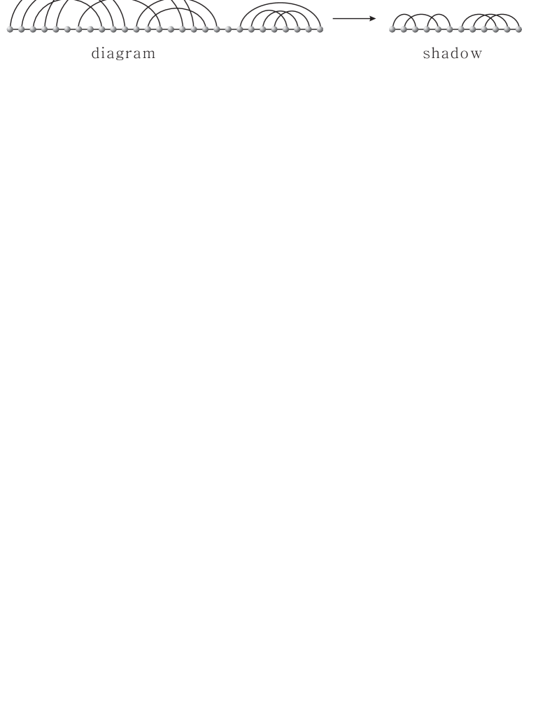
Fig. 3. Shadows: the shadow is obtained by removing all noncrossing arcs and isolated points and collapsing all stacks and resulting stacks into single arcs.

The shadow of a diagram $\mathbb{G}$, $\sigma(\mathbb{G})$, can possibly be empty. Furthermore, projecting into the shadow does not affect genus. Any shadow of genus $g$ over one backbone contains at least $2g$ and at most $(6g-2)$ arcs. In particular, for fixed genus $g$, there exist only finitely many shadows Reidys et al. (2011); Andersen et al. (2012a). In Fig. 4, we display the four shadows of genus one.

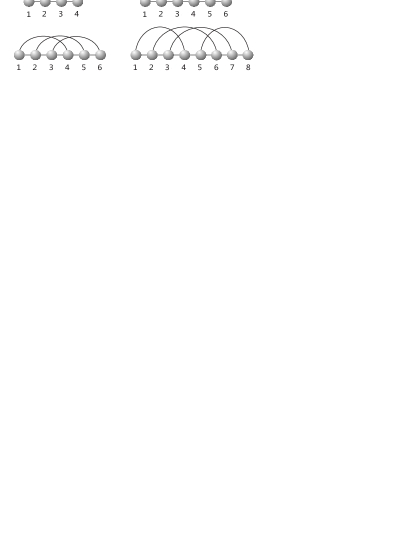
Fig. 4. The four shadows of genus one.

A diagram is called irreducible, if and only if for any two arcs, $\alpha_{1},\alpha_{k}$ contained in $E$, there exists a sequence of arcs $(\alpha_{1},\alpha_{2},\dots,\alpha_{k-1},\alpha_{k})$ such that $(\alpha_{i},\alpha_{i+1})$ are crossing. Irreducibility is equivalent to the concept of primitivity introduced by Bon et al. (2008), inspired by the work of Dyson (1949). According to Andersen et al. (2012a), for arbitrary genus $g$ and $2g\leq\ell\leq(6g-2)$, there exists an irreducible shadow of genus $g$ having exactly $\ell$ arcs. We may reuse Fig. 4 as an illustration of this result since the four shadows of genus one are all irreducible.

Let ${\bf i}_{g}(m)$ denote the number of irreducible shadows of genus $g$ with $m$ arcs. Since for fixed genus $g$ there exist only finitely many shadows we have the generating polynomial of irreducible shadows of genus $g$

$${\bf I}_{g}(z)=\sum_{m=2g}^{6g-2}\,{\bf i}_{g}(m)z^{m}.$$

For instance for genus $1$ and $2$ we have

$${\bf I}_{1}(z) = {z}^{2}\left(1+z\right)^{2},$$

$${\bf I}_{2}(z) = {z}^{4}\left(1+z\right)^{4}\left(17+92\,z+96\,{z}^{2}\right).$$

The shadow $\sigma(\mathbb{G})$ of a diagram $\mathbb{G}$ decomposes into a set of irreducible shadows. We shall call these shadows irreducible $\mathbb{G}$-shadows.

Any diagram $\mathbb{G}$ can iteratively be decomposed by first removing all noncrossing arcs as well as isolated vertices, second collapsing any stacks and third by removing irreducible $\mathbb{G}$-shadows iteratively as follows, see Fig. 5:
$\bullet$ one removes (i.e. cuts the backbone at two points and after removal merges the cut-points) irreducible $\mathbb{G}$-shadows from bottom to top, i.e. such that there exists no irreducible $\mathbb{G}$-shadow that is nested within the one previously removed.
$\bullet$ if the removal of an irreducible $\mathbb{G}$-shadow induces the formation of a stack, it is collapsed into a single arc.

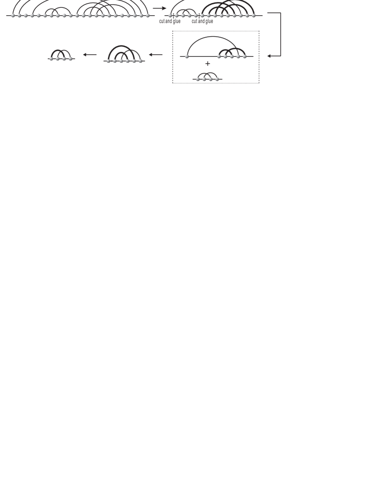
Fig. 5. A diagram $\mathbb{G}$ is decomposed: we remove any noncrossing arcs and isolated points, collapse any stacks into a single arcs and finally remove irreducible $\mathbb{G}$-shadows from bottom to top and collapsing any stack generated in the process into a single arc.

A diagram, $\mathbb{G}$, is a $\gamma$-diagram if and only if for any irreducible $\mathbb{G}$-shadow, $\mathbb{G}^{\prime}$, $g(\mathbb{G}^{\prime})\leq\gamma$ holds.

We denote the set of $\tau$-canonical $\gamma$-diagrams by $\widetilde{\mathcal{G}}_{\tau,\gamma}$. Such a diagram without arcs of the form $(i,i+1)$ ($1$-arcs) is called a $\tau$-canonical $\gamma$-structure and their set is denoted by $\mathcal{G}_{\tau,\gamma}$. A $\gamma$-matching is a $\gamma$-diagram that contains only vertices of degree three. A $\gamma$-shape is a $\gamma$-matching that contains only stacks of length zero. Let $\mathcal{H}_{\gamma}$ and $\mathcal{S}_{\gamma}$ denote the set of $\gamma$-matchings and $\gamma$-shapes, respectively.

2.2. Some generating functions

In this paper we denote the ring of polynomials over a ring $R$ by $R[X]$ and the ring of formal power series $\sum_{n\geq 0}a_{n}X^{n}$ by $R[[X]]$. $R[[X]]$ is a local ring with maximal ideal $(X)$, i.e. any power series with nonzero constant term is invertible. A Puiseux series Wall (2004) is power series in fractional powers of $X$, i.e. $\sum_{n\geq 0}a_{n}{X^{n/k}}$ for some fixed $k\in\mathbb{N}$.

We denote the generating functions of a set of diagrams $\mathcal{D}$ filtered by the number of arcs ${\bf D}(z)=\sum_{2n\geq 0}{\bf d}(n)z^{n}$. Similarly, a generating function of diagrams filtered by the length of the backbone is written as ${\bf D}(z)=\sum_{n\geq 0}{\bf d}(n)z^{n}$. In particular, the generating functions of $\gamma$-matchings and $\tau$ canonical $\gamma$-structures are given by

$${\bf H}_{\gamma}(u)=\sum_{2n\geq 0}{\bf h}_{\gamma}(n)u^{n},\quad{\bf G}_{\tau,\gamma}(z)=\sum_{n\geq 0}{\bf g}_{\tau,\gamma}(n)z^{n}.$$

Let $\mathcal{H}_{\gamma}(n,m)\supseteq\mathcal{S}_{\gamma}(n,m)$ denote the collections of all $\gamma$-matchings and $\gamma$-shapes on $2n\geq 0$ vertices containing $m\geq 0$ $1$-arcs with generating functions

$${\bf H}_{\gamma}(x,y)=\sum_{m,2n\geq 0}{\bf h}_{\gamma}(n,m)x^{n}y^{m},\quad{\bf S}_{\gamma}(x,y)=\sum_{m,2n\geq 0}{\bf s}_{\gamma}(n,m)x^{n}y^{m},$$

where ${\bf h}_{\gamma}(n,m)={\bf s}_{\gamma}(n,m)=0$ if $2\gamma>n$ or if $m>n$.

Furthermore there is a natural projection $\vartheta$ from $\gamma$-matchings to $\gamma$-shapes defined by collapsing each non-empty stack onto a single arc

$$\vartheta\colon{\mathcal{H}}_{\gamma}\to{\mathcal{S}}_{\gamma},$$

which is surjective and preserves irreducible shadows as well as the number of $1$-arcs. $\vartheta$ restricts to a surjection

$$\vartheta:\sqcup_{n\geq 0}{\mathcal{H}}_{\gamma}(n,m)\to\sqcup_{n\geq 0}{\mathcal{S}}_{\gamma}(n,m),$$

which collapses each stack to an arc and preserves any irreducible shadow and also the number $m$ of $1$-arcs.

3. Combinatorics of $\gamma$-matchings

In this section we study $\gamma$-matchings.

Theorem 1.

Let $R=\mathbb{Z}[u]$. Then the following assertions hold:
(a) the generating function of $\gamma$-matchings, ${\bf H}_{\gamma}(u)$, satisfies

(3.1) $${\bf H}_{\gamma}(u)^{-1}=1-\left(u\,{\bf H}_{\gamma}(u)+{\bf H}_{\gamma}(u)^{-1}\sum_{g\leq\gamma}\,{\bf I}_{g}\left(\frac{u\,{\bf H}_{\gamma}^{2}(u)}{1-u\,{\bf H}_{\gamma}^{2}(u)}\right)\right),$$

equivalently,

$${\bf H}_{\gamma}(u)-u\,{\bf H}_{\gamma}(u)^{2}-\sum_{g\leq\gamma}\,{\bf I}_{g}\left(\frac{u\,{\bf H}_{\gamma}^{2}(u)}{1-u\,{\bf H}_{\gamma}^{2}(u)}\right)=1.$$

In particular, there exists a polynomial $P_{\gamma}(u,X)\in R[X]$ of degree $(12\gamma-2)$, whose coefficients are sums of ${\bf I}_{g}(z)$ coefficients, such that $P_{\gamma}(u,{\bf H}_{\gamma}(u))=0$.
(b) eq. (3.1) determines ${\bf H}_{\gamma}(u)$ uniquely.

Proof.

We first prove (a). Let $\sigma$ be a fixed irreducible shadow of genus $g$ having $m$ arcs. Let $\mathcal{V}_{\sigma}$ be the set of diagrams, generated by concatenating and nesting $\sigma$.

Claim 1:

$${\bf V}_{\sigma}(u)=(1-{\bf V}_{\sigma}(u)^{-1}(u\,{\bf V}_{\sigma}(u)^{2})^{m})^{-1}.$$

To prove Claim $1$ we consider a $\mathcal{V}_{\sigma}$-diagram. Clearly, its maximal arcs are contained in $t\geq 1$ copies of $\sigma$. These arcs induce exactly $(2m-1)t$ $\sigma$-intervals, in each of which we find again an element of $\mathcal{V}_{\sigma}$, whence

$${\bf V}_{\sigma}(u)=\sum_{t\geq 0}(u^{m}{\bf V}_{\sigma}(u)^{2m-1})^{t}$$

and Claim $1$ follows.

Let $\mathcal{L}_{\sigma}$ be the set of diagrams having the fixed shape $\sigma$ obtained by inflating $\sigma$-arcs into stacks, or symbolically, $\mathcal{U}\,\times\textsc{Seq}(\mathcal{U})$. Here $\mathcal{U}$ and $\mathcal{R}=\textsc{Seq}(\mathcal{U})$ denote the classes of arcs and sequences of arcs. Clearly, the associated generating function of $\mathcal{U}\times\mathcal{R}$ is $u(1-u)^{-1}$.

Note that each $\mathcal{L}_{\sigma}$-diagram contains exactly $(2m-1)$ $\sigma$-intervals and an arbitrary number of pairs of ${P}$-intervals. Let $\mathcal{F}_{\sigma}$ denote the set of diagrams generated by concatenating and nesting $\mathcal{L}_{\sigma}$-diagrams that contain no empty $P$-intervals. Let finally $\mathcal{W}_{\sigma}$ be the set of $1$-canonical diagrams, having shapes in $\mathcal{F}_{\sigma}$.

Claim $2$.

(3.2) $${\bf W}_{\sigma}(u)^{-1}=1-{\bf W}_{\sigma}(u)^{-1}\left(\frac{\frac{u}{1-u}\,{\bf W}_{\sigma}^{2}(u)}{1-\frac{u}{1-u}\,({\bf W}_{\sigma}^{2}(u)-1)}\right)^{m}.$$

We shall construct $\mathcal{W}_{\sigma}$ using arcs, $\mathcal{U}$, sequences of arcs, $\mathcal{R}$, induced arcs, $\mathcal{N}$, and sequence of induced arcs, $\mathcal{M}$. The class $\mathcal{F}_{\sigma}$ is obtained by concatenating and nesting $\mathcal{L}_{\sigma}$-diagrams that do not contain any empty $P$-intervals, see Fig. 6.

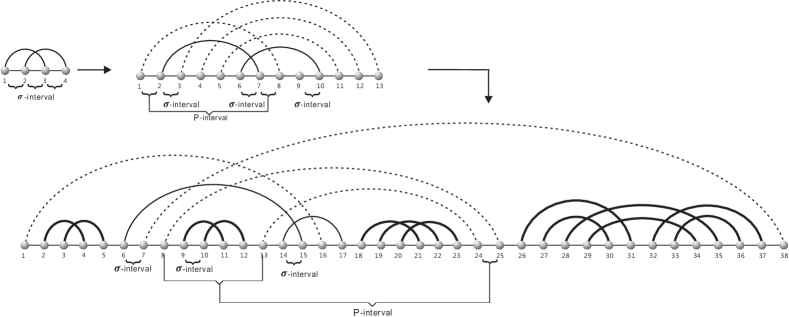
Fig. 6. First, a fixed irreducible shadow $\sigma$ is inflated into a $\mathcal{L}_{\sigma}$-diagram, second we pass to an $\mathcal{F}_{\sigma}$-diagram by inserting a nontrivial $\mathcal{L}_{\sigma}$-diagram in one of the ${P}$-intervals.

An induced arc, i.e. an arc together with at least one nontrivial $\mathcal{F}_{\sigma}$-diagram in either one or in both ${P}$-intervals

$$\mathcal{N}=\mathcal{U}\times\left((\mathcal{F}_{\sigma}-1)+(\mathcal{F}_{\sigma}-1)+(\mathcal{F}_{\sigma}-1)^{2}\right)=\mathcal{U}\times\left(\mathcal{F}_{\sigma}^{2}-1\right).$$

Clearly, we have for a single induced arc $\mathbf{N}(u)=u\left({\bf F}_{\sigma}(u)^{2}-1\right)$ and for a sequence of induced arcs, $\mathcal{M}=\textsc{Seq}(\mathcal{N})$, where

$${\bf M}(u) = \frac{1}{1-u\left({\bf F}_{\sigma}(u)^{2}-1\right)}.$$

By construction, the maximal arcs of an $\mathcal{F}_{\sigma}$-diagram coincide with those of its underlying $\mathcal{V}_{\sigma}$-diagram. Therefore

$$\mathcal{F}_{\sigma} = \sum_{t\geq 0}((\mathcal{U}\times\mathcal{M})^{m}\,\mathcal{F}_{\sigma}^{2m-1})^{t}$$

with generating function

(3.3) $${\bf F}_{\sigma}(u)=\sum_{t\geq 0}\left(\left(\frac{u}{1-u({\bf F}_{\sigma}(u)^{2}-1)}\right)^{m}\,{\bf F}_{\sigma}(u)^{2m-1}\right)^{t}.$$

Next we inflate the arcs of the $\mathcal{F}_{\sigma}$-diagram into stacks, $\mathcal{U}\,\times\mathcal{R}$.

This inflation process generates $\mathcal{W}_{\sigma}$-diagrams and any $\mathcal{W}_{\sigma}$-diagram can be constructed from a unique fixed irreducible shadow $\sigma$ of genus $g$ with $m$ arcs. We have

(3.4) $${\bf W}_{\sigma}(u)=\sum_{t\geq 0}\left(\left(\frac{\frac{u}{1-u}}{1-\frac{u}{1-u}({\bf W}_{\sigma}(u)^{2}-1)}\right)^{m}\,{\bf W}_{\sigma}(u)^{2m-1}\right)^{t},$$

whence Claim $2$.

Claim 3: Let $M$ be the set of irreducible shadows of genus $g\leq\gamma$. Then

(3.5) $${\bf W}_{M}(u)^{-1}=1-\sum_{g\leq\gamma}\sum_{1<m}{{\bf i}_{g}(m)\,\bf W}_{M}(u)^{-1}\left(\frac{u\,{\bf W}_{M}^{2}(u)}{1-u\,{\bf W}_{M}^{2}(u)}\right)^{m}.$$

The maximal arcs of a $\mathcal{V}_{M}$-structure, partition into the maximal arcs of $t$ concatenated irreducible shadows $\sigma_{1},\dots,\sigma_{t}$ and

(3.6) $$\sum_{\{\sigma_{1},\dots,\sigma_{t}\}\atop\sigma_{i}\in M}1=\left(\sum_{g\leq\gamma}\sum_{1<m}{\bf i}_{g}(m)\right)^{t}.$$

These maximal arcs induce exactly $(2m-1)\,t$ $\sigma$-intervals. In each $\sigma$-interval, we find again an element of $\mathcal{V}_{M}$. Thus for any $\sigma_{i}$ having $m$ arcs, we have $\mathcal{V}_{M}^{2m-1}$, which leads to the term $u^{m}{\bf V}_{M}(u)^{2m-1}$. It remains to sum over all $t$, i.e. expressing all the decompositions of $\mathcal{V}_{M_{\gamma}}$-structures into concatenated, irreducible shadows and we obtain

(3.7) $${\bf V}_{M}(u)=\sum_{t\geq 0}\left(\sum_{g\leq\gamma}\sum_{m>1}{\bf i}_{g}(m)u^{m}{\bf V}_{M}(u)^{2m-1}\right)^{t}.$$

The passage to from ${\mathcal{V}}_{M}$ to ${\mathcal{L}}_{M}$ as well as that from ${\mathcal{L}}_{M}$ to ${\mathcal{F}}_{M}$ follows from Claim $2$, whence

(3.8) $${\bf F}_{M}(u)=\sum_{t\geq 0}\left(\sum_{g\leq\gamma}\sum_{m>1}{{\bf i}_{g}(m)\,\bf F}_{M}(u)^{-1}\left(\frac{u\,{\bf F}_{M}^{2}(u)}{1-u\,({\bf F}_{M}^{2}(u)-1)}\right)^{m}\right)^{t}.$$

Here ${\bf F}_{M}(u)^{-1}$ exists in $\mathbb{C}[[u]]$, having a nonzero constant term. Next we inflate the arcs of the $\mathcal{F}_{M}$-structure into stacks, obtaining

(3.9) $${\bf W}_{M}(u)^{-1}=1-\sum_{g\leq\gamma}\sum_{1<m}{{\bf i}_{g}(m)\,\bf W}_{M}(u)^{-1}\left(\frac{u\,{\bf W}_{M}^{2}(u)}{1-u\,({\bf W}_{M}^{2}(u))}\right)^{m}.$$

We next derive the functional equation for $\mathbf{H}_{\gamma}(u)$ by incorporating noncrossing arcs. Since the maximal arcs composed of noncrossing arcs are exactly rainbows, the generating function of $\mathcal{H}_{\gamma}$-diagrams nested in a rainbow is given by $u\,{\bf H}_{\gamma}(u)$. As in Claim $3$ we conclude

$${\bf H}_{\gamma}(u)^{-1}=1-\sum_{g\leq\gamma}\left(u\,{\bf H}_{\gamma}(u)+{\bf H}_{\gamma}(u)^{-1}\,\sum_{m>1}{\bf i}_{g}(m)\,\vartheta(u)^{m}\right),$$

where

$$\vartheta(u)=\frac{u\,{\bf H}_{\gamma}^{2}(u)}{1-u\,{\bf H}_{\gamma}^{2}(u)}.$$

Setting $w_{u}(X)=1-u\,X^{2}$, eq. (3.1) gives rise to the polynomial

(3.10) $$P_{\gamma}(u,X)=w_{u}(X)^{\kappa_{\gamma}}(-1+X-u\,X^{2})-\sum_{g\leq\gamma}\,w_{u}(X)^{\kappa_{\gamma}}\,{\bf I}_{g}\left(\frac{u\,X^{2}}{w_{u}(X)}\right),$$

where $\kappa_{\gamma}=6\gamma-2$, $\text{\rm deg}(P_{\gamma}(u,X))=(2+2\kappa_{\gamma})$, $\left[X^{2+2\kappa_{\gamma}}\right]P_{\gamma}(u,X)=-u^{1+\kappa_{\gamma}}$ and $P_{\gamma}(u,{\bf H}_{\gamma}(u))=0$, whence (a).

It remains to prove (b). Since $M$ is the finite set of irreducible shadows of genus $g\leq\gamma$ and any such shadow has $2g\leq m\leq\kappa_{\gamma}$ arcs Andersen et al. (2012a), any $M$-shadow has $\leq\kappa_{\gamma}$ arcs. Setting $v(u)=1-u\,{\bf H}_{\gamma}^{2}(u)$, eq. (3.1) implies

$$v(u)^{\kappa_{\gamma}} = {\bf H}_{\gamma}(u)v(u)^{\kappa_{\gamma}}-u\,{\bf H}^{2}_{\gamma}(u)\,v(u)^{\kappa_{\gamma}}-\sum_{g\leq\gamma}\,v(u)^{\kappa_{\gamma}}\,{\bf I}_{g}\left(\frac{u\,{\bf H}_{\gamma}^{2}(u)}{v(u)}\right)$$

and consequently

(3.11) $$\begin{split}{\bf H}_{\gamma}(u)&=-{\bf H}_{\gamma}(u)\sum_{i=1}^{\kappa_{\gamma}}\,{\kappa_{\gamma}\choose i}1^{\kappa_{\gamma}-i}{(v(u)-1)^{i}}+u\,{\bf H}^{2}_{\gamma}(u)\,v(u)^{\kappa_{\gamma}}+v(u)^{\kappa_{\gamma}}\\ &+\sum_{g\leq\gamma}\,v(u)^{\kappa_{\gamma}}{\bf I}_{g}\left(\frac{u\,{\bf H}_{\gamma}^{2}(u)}{v(u)}\right).\end{split}$$

All coefficients of ${\bf H}_{\gamma}(u)$ in the RHS of eq. (3.11), are polynomials in $u$ of degree $\geq 1$, whence any $[z^{n}]{\bf H}_{\gamma}(u)$ for $n\geq(\kappa_{\gamma}+1)$ can be recursively computed. Accordingly, eq. (3.11) determines ${\bf H}_{\gamma}(u)$ uniquely. ∎

4. Irreducible shadows

The bivariate generating function of irreducible shadows of genus $g$ with $m$ arcs is denoted by

$${\bf I}(z,t)=\sum_{g\geq 1}{\bf I}_{g}(z)\,t^{g}=\sum_{g\geq 1}\sum_{m=2g}^{6g-2}\,{\bf i}_{g}(m)\,z^{m}t^{g}.$$

Let ${\bf c}_{g}(m)$ denote the number of matchings of genus $g$ with $m$ arcs. We have the generating function of matchings of genus $g$

$${\bf C}_{g}(z)=\sum_{m\geq 2g}\,{\bf c}_{g}(m)z^{m}.$$

The bivariate generating function of matchings of genus $g$ with $m$ arcs is denoted by

$${\bf C}(z,t)=\sum_{g\geq 0}{\bf C}_{g}(z)\,t^{g}=\sum_{g\geq 0}\sum_{m\geq 2g}\,{\bf c}_{g}(m)\,z^{m}t^{g}.$$

Theorem 2.

The generating functions ${\bf C}(z,t)$ and ${\bf I}(z,t)$ satisfy

$${\bf C}(z,t)^{-1}=1-\left(z\,{\bf C}(z,t)+{\bf C}(z,t)^{-1}{\bf I}\left(\frac{z\,{\bf C}(z,t)^{2}}{1-z\,{\bf C}(z,t)^{2}},t\right)\right),$$

equivalently,

(4.1) $${\bf C}(z,t)-z\,{\bf C}(z,t)^{2}-{\bf I}\left(\frac{z\,{\bf C}(z,t)^{2}}{1-z\,{\bf C}(z,t)^{2}},t\right)=1.$$

Proof.

We distinguish the classes of blocks into two categories characterized by the unique component containing all maximal arcs (maximal component). Namely,
$\bullet$ blocks whose maximal component contains only one arc,
$\bullet$ blocks whose maximal component is an (nonempty) irreducible matching.
In the first case, the removal of the maximal component (one arc) generates again an arbitrary matching, which translates into the term

$$z\,{\bf C}(z,t).$$

Let ${\bf T}(z,t)$ denote the (genus filtered) generating function of blocks of the second type. The decomposition of matchings into a sequence of blocks implies

$${\bf C}(z,t)^{-1}=1-\left(z\,{\bf C}(z,t)+{\bf T}(z,t)\right).$$

Let $\sigma$ be a fixed irreducible shadow of genus $g$ having $n$ arcs. Let ${\bf T}_{\sigma}(z,t)$ be the generating function of blocks, having $\sigma$ as the shadow of its unique maximal component. Then we have

$${\bf T}(z,t)=\sum_{\sigma\in\mathcal{I}}{\bf T}_{\sigma}(z,t),$$

where $\mathcal{I}$ denotes the set of irreducible shadows.

We shall construct $\mathcal{T}_{\sigma}$ in three steps using arcs, $\mathcal{R}$, sequences of arcs, $\mathcal{K}$, induced arcs, $\mathcal{N}$, sequence of induced arcs, $\mathcal{M}$, and arbitrary matchings, $\mathcal{C}$.

Step I: We inflate each arc in $\sigma$ into a sequence of induced arcs, see Fig. 7. An induced arc, i.e. an arc together with at least one nontrivial matching in either one or in both ${P}$-intervals

$$\mathcal{N}=\mathcal{R}\times\left((\mathcal{C}-1)+(\mathcal{C}-1)+(\mathcal{C}-1)^{2}\right)=\mathcal{R}\times\left(\mathcal{C}^{2}-1\right).$$

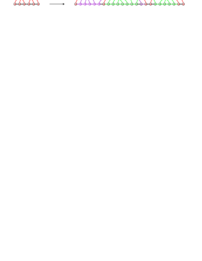
Fig. 7. Step I: inflation of each arc in $\sigma$ into a sequence of induced arcs.

Clearly, we have for a single induced arc $\mathbf{N}(z,t)=z\left({\bf C}(z,t)^{2}-1\right)$, guaranteed by the additivity of genus, and for a sequence of induced arcs, $\mathcal{M}=\textsc{Seq}(\mathcal{N})$, where

$${\bf M}(z,t) = \frac{1}{1-z\left({\bf C}(z,t)^{2}-1\right)}.$$

Inflating each arc into a sequence of induced arcs, $R^{n}\times\mathcal{M}^{n}$, gives the corresponding generating function

$$z^{n}{\bf M}(z,t)^{n}=\left(\frac{z}{1-z\left({\bf C}(z,t)^{2}-1\right)}\right)^{n},$$

since the genus is additive.

Step II: We inflate each arc in the component with shadow $\sigma$ into stacks, see Fig. 8. The corresponding generating function is

$$\left(\frac{\frac{z}{1-z}}{1-\frac{z}{1-z}\left({\bf C}(z,t)^{2}-1\right)}\right)^{n}=\left(\frac{z}{1-z{\bf C}(z,t)^{2}}\right)^{n}$$

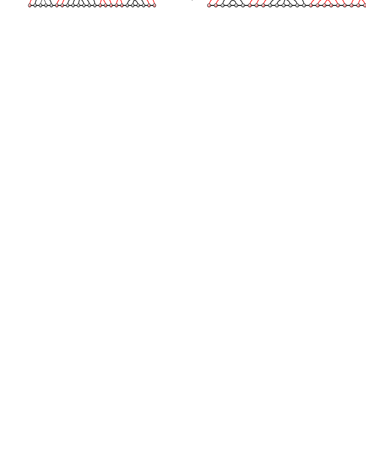
Fig. 8. Step II: inflation of each arc in the component with shadow $\sigma$ into stacks.

Step III: We insert additional matchings at exactly $(2n-1)$ $\sigma$-intervals, see Fig. 9. Accordingly, the generating function is ${\bf C}(z,t)^{2n-1}$.

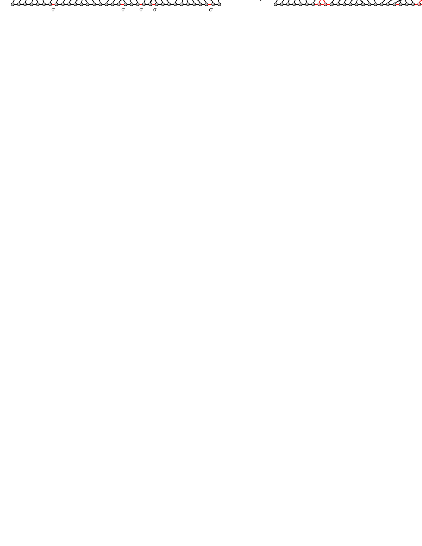
Fig. 9. Step III: insertion of additional matchings at exactly $(2n-1)$ $\sigma$-intervals.

Combining these three steps and utilizing additivity of the genus, we arrive at

$${\bf T}_{\sigma}(z,t) = t^{g}\left(\frac{z}{1-z{\bf C}(z,t)^{2}}\right)^{n}{\bf C}(z,t)^{2n-1}$$

$$= t^{g}{\bf C}(z,t)^{-1}\,\left(\frac{z{\bf C}(z,t)^{2}}{1-z{\bf C}(z,t)^{2}}\right)^{n}.$$

Therefore

$${\bf T}(z,t) = \sum_{\sigma\in\mathcal{I}}{\bf T}_{\sigma}(z,t)$$

$$= \sum_{g,n}{\bf i}_{g}(n)t^{g}\,{\bf C}(z,t)^{-1}\,\left(\frac{z{\bf C}(z,t)^{2}}{1-z{\bf C}(z,t)^{2}}\right)^{n}.$$

We derive

$${\bf T}(z,t)={\bf C}(z,t)^{-1}{\bf I}\left(\frac{z\,{\bf C}(z,t)^{2}}{1-z\,{\bf C}(z,t)^{2}},t\right),$$

completing the proof of eq. (4.1).

∎

Now we can derive a recursion for ${\bf I}_{g}(z)$ from Theorem 2.

Corollary 1.

For $g\geq 1$, ${\bf I}_{g}(z)$ satisfies the following recursion

$$\begin{split}&{\bf I}_{g}(z)={\bf C}_{g}(\theta(z))-\theta(z)\,\sum_{i=0}^{g}{\bf C}_{i}(\theta(z)){\bf C}_{g-i}(\theta(z))\\ &-\sum_{j=1}^{g-1}[t^{g-j}]{\bf I}_{j}\left(\frac{\theta(z)\,(\sum_{k=0}^{g-j}{\bf C}_{k}(\theta(z))t^{k})^{2}}{1-\theta(z)\,(\sum_{k=0}^{g-j}{\bf C}_{k}(\theta(z))t^{k})^{2}}\right),\end{split}$$

where $\theta(z)=\frac{z(z+1)}{(2z+1)^{2}}$.

Proof.

We compute the coefficient of $t^{g}$ on both sides of eq. (4.1)

$$[t^{g}]{\bf C}(t,z)-z\,[t^{g}]{\bf C}(t,z)^{2}-[t^{g}]{\bf I}\left(\frac{z\,{\bf C}(t,z)^{2}}{1-z\,{\bf C}(t,z)^{2}},t\right)=0$$

$${\bf C}_{g}(z)-z\,\sum_{i=0}^{g}{\bf C}_{i}(z){\bf C}_{g-i}(z)-\sum_{j=1}^{g}[t^{g-j}]{\bf I}_{j}\left(\frac{z\,{\bf C}(t,z)^{2}}{1-z\,{\bf C}(t,z)^{2}}\right)=0$$

$$\begin{split}&{\bf C}_{g}(z)-z\,\sum_{i=0}^{g}{\bf C}_{i}(z){\bf C}_{g-i}(z)-\sum_{j=1}^{g-1}[t^{g-j}]{\bf I}_{j}\left(\frac{z\,{\bf C}(t,z)^{2}}{1-z\,{\bf C}(t,z)^{2}}\right)\\ &=[t^{0}]{\bf I}_{g}\left(\frac{z\,{\bf C}(t,z)^{2}}{1-z\,{\bf C}(t,z)^{2}}\right)\end{split}$$

Note that

$$[t^{g-j}]{\bf I}_{j}\left(\frac{z\,{\bf C}(t,z)^{2}}{1-z\,{\bf C}(t,z)^{2}}\right)=[t^{g-j}]{\bf I}_{j}\left(\frac{z\,(\sum_{k=0}^{g-j}{\bf C}_{k}(z)t^{k})^{2}}{1-z\,(\sum_{k=0}^{g-j}{\bf C}_{k}(z)t^{k})^{2}}\right).$$

Hence,

$$\begin{split}&{\bf C}_{g}(z)-z\,\sum_{i=0}^{g}{\bf C}_{i}(z){\bf C}_{g-i}(z)-\sum_{j=1}^{g-1}[t^{g-j}]{\bf I}_{j}\left(\frac{z\,(\sum_{k=0}^{g-j}{\bf C}_{k}(z)t^{k})^{2}}{1-z\,(\sum_{k=0}^{g-j}{\bf C}_{k}(z)t^{k})^{2}}\right)\\ &={\bf I}_{g}\left(\frac{z\,{\bf C}_{0}(z)^{2}}{1-z\,{\bf C}_{0}(z)^{2}}\right)\end{split}$$

Setting $y=\frac{z\,{\bf C}_{0}(z)^{2}}{1-z\,{\bf C}_{0}(z)^{2}}$, we have $z=\theta(y)=\frac{y(y+1)}{(2y+1)^{2}}$. Then we derive

$$\begin{split}&{\bf I}_{g}(y)={\bf C}_{g}(\theta(y))-\theta(y)\,\sum_{i=0}^{g}{\bf C}_{i}(\theta(y)){\bf C}_{g-i}(\theta(y))\\ &-\sum_{j=1}^{g-1}[t^{g-j}]{\bf I}_{j}\left(\frac{\theta(y)\,(\sum_{k=0}^{g-j}{\bf C}_{k}(\theta(y))t^{k})^{2}}{1-\theta(y)\,(\sum_{k=0}^{g-j}{\bf C}_{k}(\theta(y))t^{k})^{2}}\right)\end{split}$$

completing the proof. ∎

A seminal result due to Harer and Zagier (1986), computes a recursion and generating function for the number ${\bf c}_{g}(m)$ as follows :

Lemma 1.

Harer and Zagier (1986) The ${\bf c}_{g}(m)$ satisfy the recursion

(4.2) $$(m+1)\,\mathbf{c}_{g}(m)=2(2m-1)\,\mathbf{c}_{g}(m-1)+(2m-1)(m-1)(2m-3)\,\mathbf{c}_{g-1}(m-2),$$

where $\mathbf{c}_{g}(m)=0$ for $2g>m$.

The recursion eq. (4.2) is equivalent to the ODE

(4.3) $$z(1-4z)\frac{d}{dz}\mathbf{C}_{g}(z)+(1-2z)\mathbf{C}_{g}(z) = \Phi_{g-1}(z),$$

where

$$\begin{split}&\Phi_{g-1}(z)=\\ &z^{2}\left(4z^{3}\frac{d^{3}}{dz^{3}}\mathbf{C}_{g-1}(z)+24z^{2}\frac{d^{2}}{dz^{2}}\mathbf{C}_{g-1}(z)+27z\frac{d}{dz}\mathbf{C}_{g-1}(z)+3\mathbf{C}_{g-1}(z)\right)\end{split}$$

with initial condition $\mathbf{C}_{g}(0)=0$ since $r=n+1-2g$ has no positive solution $r>0$ for $n<2g$. Therefore we can recursively compute $\mathbf{C}_{g}(z)$ by solving eq. (4.3) via Maple.

Theorem 3.

Andersen et al. (2012b) For any $g\geq 1$ the generating function ${\bf C}_{g}(z)$ is given by

(4.4) $$\mathbf{C}_{g}(z)=\,Q_{g}(z)\frac{\sqrt{1-4\,z}}{(1-4z)^{3g}},$$

where $Q_{g}(z)$ is a polynomial with integral coefficients of degree at most $(3g-1)$, $Q_{g}(1/4)\neq 0$, $[z^{2g}]Q_{g}(z)\neq 0$ and $[z^{h}]Q_{g}(z)=0$ for $0\leq h\leq 2g-1$.

The recursion eq. (4.3) permits the calculation of the polynomials $Q_{g}(z)$, the first five of which are given as follows Andersen et al. (2012b)

$$Q_{1}(z) = z^{2},$$

$$Q_{2}(z) = 21z^{4}\,\left(z+1\right)$$

$$Q_{3}(z) = 11z^{6}\,\left(158\,{z}^{2}+558\,z+135\right),$$

$$Q_{4}(z) = 143z^{8}\left(2339\,{z}^{3}+18378\,{z}^{2}+13689\,z+1575\right),$$

$$Q_{5}(z) = 88179z^{10}\,\left(1354\,{z}^{4}+18908\,{z}^{3}+28764\,{z}^{2}+9660\,z+675\right).$$

Applying Corollary 1 together with the generating function ${\bf C}_{g}(z)$, we recursively compute ${\bf I}_{g}(z)$.

For example, for $g=1$,

$${\bf I}_{1}(z) = {\bf C}_{1}(\theta(z))-2\theta(z)\,{\bf C}_{0}(\theta(z)){\bf C}_{1}(\theta(z))$$

$$= {z}^{2}\left(1+z\right)^{2}.$$

For $1\leq g\leq 8$, we list ${\bf I}_{g}(z)$ as follows

$${\bf I}_{1}(z) = {z}^{2}\left(1+z\right)^{2},$$

$${\bf I}_{2}(z) = {z}^{4}\left(1+z\right)^{4}\left(17+92\,z+96\,{z}^{2}\right)$$

$${\bf I}_{3}(z) = {z}^{6}\left(1+z\right)^{6}\left(1259+15928\,z+61850\,{z}^{2}+92736\,{z}^{3}+47040\,{z}^{4}\right)$$

$${\bf I}_{4}(z) = {z}^{8}\left(1+z\right)^{8}\left(200589+4245684\,z+31264164\,{z}^{2}+107622740\,{z}^{3}\right.$$

$$\left.+188262816\,{z}^{4}+161967360\,{z}^{5}+54333440\,{z}^{6}\right)$$

$${\bf I}_{5}(z) = {z}^{10}\left(1+z\right)^{10}\left(54766516+1681752448\,z+19092044658\,{z}^{2}\right.$$

$$+109184482584\,{z}^{3}+353376676011\,{z}^{4}$$

$$+675135053568\,{z}^{5}+753610999040\,{z}^{6}$$

$$\left.+453941596160\,{z}^{7}+113867919360\,{z}^{8}\right)$$

$${\bf I}_{6}(z) = 3\,{z}^{12}\left(1+z\right)^{12}\left(7613067765+312905543772\,z+4932317894440\,{z}^{2}\right.$$

$$+40797413383380\,{z}^{3}+200964285178270\,{z}^{4}+626595744773516\,{z}^{5}$$

$$+1268150755326432\,{z}^{6}+1660845652501760\,{z}^{7}+1357241056522240\,{z}^{8}$$

$$\left.+628740761518080\,{z}^{9}+126004558299136\,{z}^{10}\right)$$

$${\bf I}_{7}(z) = {z}^{14}\left(1+z\right)^{14}\left(13532959408258+706557271551408\,z\right.$$

$$+14506513039164060\,{z}^{2}+160434554727348896\,{z}^{3}$$

$$+1089075339931680039\,{z}^{4}+4857650169218369856\,{z}^{5}$$

$$+14771712773087154704\,{z}^{6}+31138771188689736192\,{z}^{7}$$

$$+45486763075779571200\,{z}^{8}+45167296685229793280\,{z}^{9}$$

$$+29078583024627105792\,{z}^{10}$$

$$\left.+10941912454886326272\,{z}^{11}+1826131581135486976\,{z}^{12}\right)$$

$${\bf I}_{8}(z) = {z}^{16}\left(1+z\right)^{16}\left(10826939105517381+692156096364848676\,z\right.$$

$$+17724869034206737356\,{z}^{2}$$

$$+249069951630509297956\,{z}^{3}+2192230050291936695620\,{z}^{4}$$

$$+12980362620620450943588\,{z}^{5}+53923920139564145104556\,{z}^{6}$$

$$+161060520394034807160164\,{z}^{7}+349969438514715552162336\,{z}^{8}$$

$$+553647075623879302120960\,{z}^{9}+630641488385967162351616\,{z}^{10}$$

$$+503519879227179011162112\,{z}^{11}+267275771110990512783360\,{z}^{12}$$

$$\left.+84670509266097640833024\,{z}^{13}+12107536630199227514880\,{z}^{14}\right)$$

We conjecture that the polynomial ${\bf I}_{g}(z)$, for arbitrary $g$, has ${z}^{2g}\left(1+z\right)^{2g}$ as a factor.

5. Asymptotics of $\gamma$-matchings

Let us begin recalling the following result of Flajolet and Sedgewick (2009):

Theorem 4.

Let $y(u)=\sum_{n\geq 0}y_{n}u^{n}$ be a generating function, analytic at $0$, satisfy a polynomial equation $\Phi(u,y)=0$. Let $\rho$ be the real dominant singularity of $y(u)$. Define the resultant of $\Phi(u,y)$ and $\frac{\partial}{\partial y}\Phi(u,y)$ as polynomial in $y$

$$\Delta(u)=\mathbf{R}\left(\Phi(u,y),\frac{\partial}{\partial y}\Phi(u,y),y\right).$$

(1) The dominant singularity $\rho$ is unique and a root of the resultant $\Delta(u)$ and there exists $\pi=y(\rho)$, satisfying the system of equations,

(5.1) $$\Phi(\rho,\pi)=0,\quad\Phi_{y}(\rho,\pi)=0.$$

(2) If $\Phi(u,y)$ satisfies the conditions:

(5.2) $$\Phi_{u}(\rho,\pi)\neq 0,\quad\Phi_{yy}(\rho,\pi)\neq 0,$$

then $y(u)$ has the following expansion at $\rho$

(5.3) $$y(u)=\pi+\lambda(\rho-u)^{\frac{1}{2}}+O(\rho-u),\quad\text{for some nonuero constant }\lambda.$$

Further the coefficients of $y(u)$ satisfy

$$[u^{n}]y(u)\sim c\,n^{-\frac{3}{2}}\rho^{-n},\quad n\rightarrow\infty,$$

for some constant $c>0$.

Proof.

The proof of (1) can be found in Flajolet and Sedgewick (2009) or Hille (1962) pp. 103. To prove (2), let $\Psi(u,y)=\Phi(\rho-u,\pi-y)$. Immediately, we have $\Psi(0,0)=0$. Puiseux’s Theorem Wall (2004) guarantees a solution of $y-\pi$ in terms of a Puiseux series in $\rho-u$. Note that equations (5.1) and (5.2) are equivalent to

$$\Psi(0,0)=0,\quad\Psi_{y}(0,0)=0,\quad\Psi_{u}(0,0)\neq 0,\quad\Psi_{yy}(0,0)\neq 0.$$

Then we apply Newton’s polygon method to determine the type of expansion and find the first exponent of $u$ to be $\frac{1}{2}$. Therefore the Puiseux series expansion of $y(u)$ has the required form. The asymptotics of the coefficients follows from eq. (5.3) as a straightforward application of the transfer theorem (Flajolet and Sedgewick (2009), pp. 389 Theorem VI.3). ∎

Combining Theorem 1 and Theorem 4, the asymptotic analysis of ${\bf H}_{\gamma}(u)$ follows.

Theorem 5.

For $1\leq\gamma\leq 10$, let

$$\Delta_{\gamma}(u)=\mathbf{R}\left(P_{\gamma}(u,X),\frac{\partial}{\partial X}P_{\gamma}(u,X),X\right)$$

the resultant of $P_{\gamma}(u,X)$ and $\frac{\partial}{\partial X}P_{\gamma}(u,X)$ as polynomials in $X$, and $\rho_{\gamma}$ denote the real dominant singularity of ${\bf H}_{\gamma}(u)$.
(a) the dominant singularity $\rho_{\gamma}$ is unique and a root of $\Delta_{\gamma}(u)$,
(b) at $\rho_{\gamma}$ we have

$${\bf H}_{\gamma}(u)=\pi_{\gamma}+\lambda_{\gamma}(\rho_{\gamma}-u)^{\frac{1}{2}}+O(\rho_{\gamma}-u),\quad\text{for some nonuero constant }\lambda_{\gamma}.$$

(c) the coefficients of ${\bf H}_{\gamma}(u)$ are asymptotically given by

$$[u^{n}]{\bf H}_{\gamma}(u) \sim c_{\gamma}\,n^{-3/2}\,\rho_{\gamma}^{-n}$$

for some $c_{\gamma}>0$.

Proof.

Pringsheim s Theorem (Flajolet and Sedgewick (2009) pp. 240) guarantees that for any $\gamma$, ${\bf H}_{\gamma}(u)$ has a dominant real singularity $\rho_{\gamma}>0$. To prove the singular expansion of the function and asymptotic of the coefficients, we verify $P_{\gamma}(u,X)$, for $1\leq\gamma\leq 10$, satisfy the condition of Theorem 4 and the results follow. ∎

6. Combinatorics of $\gamma$-diagrams

Lemma 2.

For any $\gamma\geq 1$, we have

(6.1) $${\bf S}_{\gamma}(u,e) = \frac{1+u}{1+2u-ue}{\bf H}_{\gamma}\left(\frac{u(1+u)}{(1+2u-ue)^{2}}\right).$$

The proof of Lemma 2 can be obtained by standard symbolic method.

Lemma 3.

Let $\lambda$ be a fixed $\gamma$-shape with $s\geq 1$ arcs and $m\geq 0$ 1-arcs. Then the generating function of $\tau$-canonical $\gamma$-diagrams containing no $1$-arc that have shape $\lambda$ is given by

$${\bf G}^{\lambda}_{\tau,\gamma}(z)=(1-z)^{-1}\left(\frac{z^{2\tau}}{(1-z^{2})(1-z)^{2}-(2z-z^{2})z^{2\tau}}\right)^{s}\,z^{m}.$$

In particular, ${\bf G}^{\lambda}_{\tau,\gamma}(z)$ depends only upon the number of arcs and $1$-arcs in $\lambda$.

Our main result about enumerating $\tau$-canonical $\gamma$-structures follows.

Theorem 6.

Suppose $\gamma,\tau\geq 1$ and let $u_{\tau}(z)=\frac{(z^{2})^{\tau-1}}{z^{2\tau}-z^{2}+1}$. Then the generating function ${\bf G}_{\tau,\gamma}(z)$ is algebraic and given by

(6.2) $${\bf G}_{\tau,\gamma}(z) = \frac{1}{u_{\tau}(z)z^{2}-z+1}\ {\bf H}_{\gamma}\left(\frac{u_{\tau}(z)z^{2}}{\left(u_{\tau}(z)z^{2}-z+1\right)^{2}}\right).$$

In particular for $1\leq s,i\leq 2$ we have

$$[z^{n}]{\bf G}_{s,i}(z)\sim k_{s,i}\,n^{-\frac{3}{2}}(\rho_{s,i}^{-1})^{n},\quad$$

for some constants $k_{s,i}>0$, for $\rho_{s,i}^{-1}$, we have Table 1.

Proof.

Since each $\gamma$-diagram has a unique $\gamma$-shape, $\lambda$, having some number $m\geq 0$ of $1$-arcs, we have

(6.3) $${\bf G}_{\tau,\gamma}(z)=\sum_{m\geq 0}\sum_{\lambda\,\text{\rm$\gamma$-shape}\atop\text{\rm having $m$ $1$-arcs}}\mathbf{G}^{\lambda}_{\tau,\gamma}(z).$$

According to Lemma 3, ${\bf G}^{\lambda}_{\tau,\gamma}(z)$ only depends on the number of arcs and $1$-arcs of $\lambda$, and we can therefore express

$${\bf G}_{\tau,\gamma}(z) = {1\over{z-1}}~{}{\bf S}_{\gamma}\biggl{(}{{z^{2\tau}}\over{(1-z^{2})(1-z)^{2}-(2z-z^{2})z^{2\tau}}},z\biggr{)}$$

$$= \frac{1}{(1-z)+{u_{\tau}(z)}z^{2}}\,{\bf H}_{\gamma}\left(\frac{z^{2}\,{u_{\tau}(z)}}{\bigl{(}(1-z)+{u_{\tau}(z)}z^{2}\bigr{)}^{2}}\right),$$

using Lemma 2 in order to confirm eq. (6.5), where the second equality follows from direct computation. Let

$$\theta_{\tau}(z)=\frac{z^{2}\,{u_{\tau}(z)}}{\bigl{(}(1-z)+{u_{\tau}(z)}z^{2}\bigr{)}^{2}}$$

denote the argument of ${\bf H}_{\gamma}$ in this expression. By definition we have $\theta(z)\in\mathbb{C}(z)$. Since $\theta_{\sigma}(0)=0$ the composition ${\bf H}_{\gamma}(\theta(z))$ is welldefined as a powerseries. Obviously, $P_{\gamma}(z,\mathbf{H}_{\gamma}(z))=0$ guarantees $P_{\gamma}(\theta_{\tau}(z),{\bf H}_{\gamma}(\theta_{\tau}(z))=0$. We have the following Hasse diagram of fields

from which we immediately conclude that ${\bf G}_{\tau,\gamma}(z)$ is algebraic. Pringsheim’s Theorem Flajolet and Sedgewick (2009) guarantees that for any $\gamma,\tau\geq 1$, ${\bf G}_{\tau,\gamma}(z)$ has a dominant real singularity $\rho_{\tau,\gamma}>0$.

According to Theorem 5 we have

$$\mathbf{H}_{i}(z)=\pi_{1}+\sum_{j\geq 1}a_{j,i}\left(\left(\mu_{i}-z\right)^{1/2}\right)^{j}\quad\text{\rm and}\quad[z^{n}]\mathbf{H}_{i}(z)\sim k_{i}\;n^{-3/2}\;\left(\mu_{i}^{-1}\right)^{n}.$$

For $\tau=1,2$, we verify directly that $\rho_{1,i}$ and $\rho_{2,i}$ are the unique solutions of minimum modulus of $\theta_{1}(z)=\mu_{i}$ and $\theta_{2}(z)=\mu_{i}$. These solutions are strictly smaller than any other singularities of $\theta_{1}(z)$ and $\theta_{2}(z)$ and furthermore satisfy $\theta_{1}^{\prime}(\rho_{1,i})\neq 0$ as well as $\theta_{2}^{\prime}(\rho_{2,i})\neq 0$. It follows that ${\bf G}_{1,i}(z)$ and ${\bf G}_{2,i}(z)$ are governed by the supercritical paradigm Flajolet and Sedgewick (2009), which in turn implies

(6.4) $$[z^{n}]\mathbf{G}_{s,i}(z)\sim k_{s,i}\,n^{-3/2}\left(\rho_{s,i}^{-1}\right)^{n}$$

where $s=1,2$ and $k_{s,i}$ is some positive constant. ∎

Theorem 6 has its analogue for $\tau$-canonical, $\gamma$-diagrams containing $1$-arcs. The asymptotic formula in case of $\tau=1,\gamma=1$,

$$[z^{n}]\widetilde{{\bf G}}_{1,1}(z)\sim j_{1}\,n^{-\frac{3}{2}}(\varrho_{1,1}^{-1})^{n}$$

is due to Nebel and Weinberg (2011) who used the explicit grammar developed in Reidys et al. (2011) in order to obtain an algebraic equation for $\widetilde{{\bf G}}_{1,1}(z)$.

Corollary 2.

Suppose $\gamma,\tau\geq 1$ and let $u_{\tau}(z)=\frac{(z^{2})^{\tau-1}}{z^{2\tau}-z^{2}+1}$. Then the generating function of $\tau$-canonical $\gamma$-diagrams containing $1$-arcs, $\widetilde{{\bf G}}_{\tau,\gamma}(z)$, is algebraic and

(6.5) $$\widetilde{{\bf G}}_{\tau,\gamma}(z) = {\bf H}_{\gamma}\left(\frac{u_{\tau}(z)z^{2}}{(1-z)^{2}}\right).$$

In particular for $\gamma=1$ we have

$$[z^{n}]\widetilde{{\bf G}}_{1,1}(z)\sim j_{1}\,n^{-\frac{3}{2}}(\varrho_{1,1}^{-1})^{n},\quad\text{\rm and}\quad[z^{n}]\widetilde{{\bf G}}_{2,1}(z)\sim j_{2}\,n^{-\frac{3}{2}}(\varrho_{2,1}^{-1})^{n}$$

for some constants $j_{1},j_{2}$, where $\varrho_{1,1}^{-1}=3.8782$ and $\varrho_{2,1}^{-1}=2.3361$.

Proof.

Let $\lambda$ be a fixed $\gamma$-shape with $s\geq 1$ arcs and $m\geq 0$ 1-arcs. Then the generating function of $\tau$-canonical $\gamma$-diagrams containing $1$-arcs that have shape $\lambda$ containing 1-arcs is given by

$$\widetilde{{\bf G}}_{\tau,\gamma}(z)=(1-z)^{-1}\left(\frac{z^{2\tau}}{(1-z^{2})(1-z)^{2}-(2z-z^{2})z^{2\tau}}\right)^{s}.$$

∎

7. Discussion

The symbolic approach based on $\gamma$-matchings allows not only to compute the generating function of canonical $\gamma$-structures. On the basis of Theorem 6 it is possible to obtain a plethora of statistics of $\gamma$-structures by means of combinatorial markers.

For instance, we can analogously compute the bivariate generating function of $\tau$ canonical $\gamma$-structures over $n$ vertices, containing exactly $m$ arcs, ${\bf A}_{\tau,\gamma}(z,t)$ as

(7.1) $${\bf A}_{\tau,\gamma}(z,t)=\frac{1}{u_{\tau}(z,t)z^{2}-z+1}{\bf H}_{\gamma}\left(\frac{u_{\tau}(z,t)\;z^{2}}{(u_{\tau}(z,t)z^{2}-z+1)^{2}}\right)$$

where $u_{\tau}(z,t)$ is given by

$$u_{\tau}(z,t)=\frac{t\,(tz^{2})^{\tau-1}}{(tz^{2})^{\tau}-tz^{2}+1}\ .$$

This bivariate generating function is the key to obtain a central limit theorem for the distribution of arc-numbers in $\gamma$-structures Bender (1973) on the basis of Lévy-Cramér Theorem on limit distributions Feller (1991).

Statistical properties of $\gamma$-structures play a key role for quantifying algorithmic improvements via sparsifications Busch et al. (2008); Möhl et al. (2010); Wexler (2007). The key property here is the polymer-zeta property Kabakcioglu and Stella (2008); Kafri et al. (2000) which states that the probability of an arc of length $\ell$ is bounded by $k\,\ell^{c}$, where $k$ is some positive constant and $c>1$. Polymer-zeta stems from the theory of self-avoiding walks Vanderzande (1998) and has only been empirically established for the simplest class of RNA structures, namely those of genus zero. It turns out however, that the polymer-zeta property is genuinely a combinatorial property of a structure class. Moreover our results allow to quantify the effect of sparsifications of folding algorithms into $\gamma$-structures Andersen et al. (2012a); Huang and Reidys (2012).

We finally remark that around 98% of RNA pseudoknot structures catalogued in databases are in fact canonical $1$-structures. RNA pseudoknot structures like the HDV-virus exhibiting irreducible shadows of genus two are relatively rare.

Acknowledgments. We want to thank Fenix W.D. Huang for discussions and comments. We furthermore acknowledge the financial support of the Future and Emerging Technologies (FET) programme within the Seventh Framework Programme (FP7) for Research of the European Commission, under the FET-Proactive grant agreement TOPDRIM, number FP7-ICT-318121.

Table 1. The exponential growth rates of $\rho_{s,i}^{-1}$, for $1\leq s,i\leq 2$.

$(s,i)$	$(1,1)$	$(2,1)$	$(1,2)$	$(2,2)$
$\rho_{s,i}^{-1}$	3.6005	2.2759	3.8846	2.3553

References

- Andersen et al. (2012a) Andersen, J.E., Huang, F.W.D., Penner, R.C., et al. Topology of RNA-interaction structures. J. Comput. Biol., 19:928–943, 2012.
- Andersen et al. (2012b) Andersen, J.E., Penner, R.C., Reidys, C.M., et al. Topological classification and enumeration of rna structures by genus. J. Math. Bio. Accepted.
- Bailor et al. (2010) Bailor, M.H., Sun, X., Al-Hashimi, H.M. Topology links RNA secondary structure with global conformation, dynamics, and adaptation. Science, 327:202–206, 2010.
- Bender (1973) E.A. Bender. Central and local limit theorems applied to asymptotic enumeration. J. Combin. Theory A, 15:91–111, 1973.
- Bon et al. (2008) Bon, M., Vernizzi, G., Orland, H., et al. Topological classification of RNA structures. J. Mol. Biol., 379:900–911, 2008.
- Busch et al. (2008) Busch, A., Richter, A.S., Backofen, R. IntaRNA: efficient prediction of bacterial sRNA targets incorporating target site accessibility and seed regions. Bioinformatics, 24:2849–2856, 2008.
- Dyson (1949) Dyson, F.J. The S matrix in quantum electrodynamics. Phys. Rev., 75:1736–1755, 1949.
- Feller (1991) Feller, W. An Introduction to Probability Theory and Its Application. Addison-Wesley Publishing Company Inc., NY, 1991.
- Flajolet and Sedgewick (2009) Flajolet, P., and Sedgewick, R. Analytic Combinatorics. Cambridge University Press New York, 2009.
- Harer and Zagier (1986) Harer, J., and Zagier, D. The euler characteristic of the moduli space of curves. Invent. Math., 85:457–486, 1986.
- Hille (1962) Hille, E. Analytic Function Theory, Volume II. Chelsea Publishing Company, 1962.
- Huang and Reidys (2012) Huang, F.W.D., and Reidys, C.M. On the combinatorics of sparsification. Algorithm. Mol. Biol., 7:28, 2012.
- Kabakcioglu and Stella (2008) Kabakcioglu, A., and Stella, A.L. A scale-free network hidden in the collapsing polymer. Bioinformatics, 2008. ArXiv Condensed Matter e-prints.
- Kafri et al. (2000) Kafri, Y., Mukamel, D., Peliti, L. Why is the DNA denaturation transition first order? Phys. Rev. Lett., 85:4988–4991, 2000.
- Loebl and Moffatt (2008) Loebl, M., and Moffatt, I. The chromatic polynomial of fatgraphs and its categorification. Adv. Math., 217:1558–1587, 2008.
- Massey (1967) Massey, W.S. Algebraic Topology: An Introduction. Springer-Veriag, New York, 1967.
- Mathews et al. (1999) Mathews, D., Sabina, J., Zuker, M., et al. Expanded sequence dependence of thermodynamic parameters improves prediction of RNA secondary structure. J. Mol. Biol., 288:911–940, 1999.
- Möhl et al. (2010) Möhl, R., Salari, R., Will, S., et al. Sparsification of RNA structure prediction including pseudoknots. Algorithms for Molecular Biology, 5:39, 2010.
- Nebel and Weinberg (2011) Nebel, M.E., and Weinberg, F. Algebraic and combinatorial properties of common RNA pseudoknot classes with applications. 2011.
- Orland and Zee (2002) Orland, H., and Zee, A. RNA folding and large matrix theory. Nuclear Physics B, 620:456–476, 2002.
- Penner (2004) Penner, R.C. Cell decomposition and compactification of Riemann’s moduli space in decorated Teichmüller theory. In Nils Tongring and R.C. Penner, editors, Woods Hole Mathematics-perspectives in math and physics, pages 263–301. World Scientific, Singapore, 2004. arXiv: math. GT/0306190.
- Penner et al. (2010) Penner, R.C., Knudsen, M., Wiuf, C., et al. Fatgraph models of proteins. Comm. Pure Appl. Math., 63:1249–1297, 2010.
- Penner and Waterman (1993) Penner, R.C., and Waterman, M.S. Spaces of rna secondary structures. Adv. Math., 101:31–49, 1993.
- Reidys et al. (2011) Reidys, C.M., Huang, F.W.D., Andersen, J.E., et al. Topology and prediction of RNA pseudoknots. Bioinformatics, 27:1076–1085, 2011.
- Smith and Waterman (1978) Smith, T.F., and Waterman, M.S. RNA secondary structure. Math. Biol., 42:31–49, 1978.
- Tabaska et al. (1998) Tabaska, J.E., Cary, R.B., Gabow, H.N., et al. An RNA folding method capable of identifying pseudoknots and base triples. Bioinformatics, 14:691–699, 1998.
- Vanderzande (1998) Vanderzande, C. Lattice Models of Polymers. Cambridge University Press, New York, 1998.
- Wall (2004) Wall, C.T.C. Singular Points of Plane Curves. Cambridge University Press, 2004.
- Wexler (2007) Wexler, Y., Zilberstein, C., Ziv-ukelson, M. A study of accessible motifs and RNA folding complexity. J. Comput. Biol., 14:6, 2007.