Thermoelectric effect in a parallel double quantum dot structure

Abstract

We discuss the thermoelectric properties assisted by the Fano effect of a parallel double quantum dot (QD) structure. By adjusting the couplings between the QDs and leads, we facilitate the nonresonant and resonant channels for the Fano interference. It is found that at low temperature, Fano lineshapes appear in the electronic and thermal conductance spectra, which can also be reversed by an applied local magnetic flux with its phase factor $\phi=\pi$. And, the Fano effect contributes decisively to the enhancement of thermoelectric efficiency. However, at the same temperature, the thermoelectric effect in the case of $\phi=\pi$ is much more apparent, compared with the case of zero magnetic flux. By the concept of Feynman path, we analyze the difference between the quantum interferences in the cases of $\phi=0$ and $\phi=\pi$. It is seen that in the absence of magnetic flux the Fano interference originates from the quantum interference among infinite-order Feynman paths, but it occurs only between two lowest-order Feynman paths when $\phi=\pi$. The increase of temperature inevitably destroys the electron coherent transmission in each paths. So, in the case of zero magnetic field, the thermoelectric effect contributed by the Fano interference is easy to weaken by a little increase of temperature.

I Introduction

The field of thermoelectricity and solid-state thermionics has recently received renewed attention, due to advances in growth and fabrication of complex compounds, mesoscopic devices and nanostructures.RMP1 ; ZhangC The main purpose is to enhance the efficiency of solid-state thermoelectric devices at a mesoscopic or nanoscopic scale.ChenG As is known, the thermoelectric efficiency of a solid-state device is described by the figure of merit $ZT$. $ZT$ is defined as

$$ZT=S^{2}{\cal G}T/\kappa,$$ (1)

where $S$, $\cal G$, and $T$ are thermopower, electronic conductance, and absolute temperature, respectively. $\kappa=\kappa_{el}+\kappa_{ph}$ is the thermal conductance, in which $\kappa_{el}$ is the electron and $\kappa_{ph}$ the phonon thermal conductance.Mahan Besides, the thermal and electronic conductances for most macroscopic metals at very low or room temperatures are constrained by the Wiedemann-Franz law,

$$\kappa/{\cal G}T=L_{0},$$ (2)

where $L_{0}=k_{B}^{2}\pi^{3}/3e^{2}$ is the Lorenz number with $k_{B}$ the Boltzmann constant and $e$ the electron charge.Grosso Since the relationship between these parameters above, it is difficult to achieve the increment of thermoelectric efficiency in bulk materials.

The progress of research on the quantum transport through mesoscopic systems and nanostructures motivates scientists to pay close attention to the thermoelectric properties of mesoscale or nanosale structures.Science1 Recently, there reported a number of interesting experimental results, and the barrier of $ZT=1$ has been overcome at high temperatures in such structures. Harman $et$ $al.$ observed $ZT\simeq 1.6$ in a $\rm{PbSeTe}$ based quantum dot superlattice.Herman Venkatasubramanian $et$ $al.$ achieved $ZT\approx 2.4$ in a p-type $\rm{Bi_{2}Te_{3}/Sb_{2}Te_{3}}$ superlattice.Siivola More recently, Kanatzidis and co-workers found that bulk $\rm{AgPb_{18}SbTe_{20}}$ with internal nanostructures has $ZT\approx 2$ at $T=800K$.Hsu In nanocrystalline $\rm{BiSbTe}$ bulk alloys $ZT$ reached the value 1.4 at $T=373K$.Poudel And, a 100-fold improvement of $ZT$ compared to the bulk value has been reported lately in $\rm{Si}$ nanowires.ChenR ; Boukai On the other hand, Lyeo $et$ $al.$ measured the Seebeck coefficient across a junction formed by a semiconducting substrate and the tip of a scanning transmission microscope. The consensus is that finding a material with a thermoelectric figure of merit $ZT\geq 4$ would mark a major technological breakthrough.Lyeo The experimental results were well explained by theoretical workers. It was found that the enhanced $ZT$ in nanostructures is attributed to the decrease of the thermal conductance produced by the scattering of phonons off the structure,Hicks ; Wang or due to the increase of thermopower induced by the presence of enhanced densities of states at the Fermi level.Zeitler ; Oxford ; Mahan2

QD systems are typical nanostructures, since they contain a variety of interesting quantum transport properties with their potential applications. Furthermore, based on the work of Mahan and Sofo,Mahan2 it can be anticipated that QDs and molecular junctions are good candidates to explore the thermoelectric properties of low-dimensional structures, since the $\delta$-like density of states and small phonon contribution to thermal conductance in these systems.Hicks ; Mahan2 ; Triberis Consequently, many experimental and theoretical groups have devoted themselves to the thermoelectric properties of QDs and molecules, as a result, some interesting phenomena were reported.Staring ; Bruder ; Koch ; Kubala ; Zianni ; Fazio ; DongB ; Kraw ; Kita ; Reuter ; Yosida ; Nguyen ; Triberis ; Barnas First, it was found that in these systems, the characteristics of level quantization and Coulomb blockade effects indeed lead to novel thermoelectric features, such as oscillations of the thermopower and oscillations of the thermal conductance.Staring ; Bruder ; Zianni ; XingDY ; Sunqf On the other hand, the Coulomb interactions in QD devices have a significant influence on thermoelectric transport coefficients, and lead to strong violation of the Wiedeman-Franz law.Kubala ; Costi Experiments performed on QDs in the Kondo regime reveal a strong influence of spin correlations on the thermopower.Reuter Also, Murphy $et$ $al.$ demonstrated that violation of the Wiedeman-Franz law is the main mechanism of an enhanced thermoelectric efficiency in molecular junctions, which can be important for possible applications in energy conversion devices.Moore Then, the above results confirm that the peculiar properties of QDs play important roles in the change of thermoelectric properties.

As is known, QDs have important characteristics that some QDs can be coupled to form coupled-QD systems. In comparison with the single-QD system, coupled QDs present more intricate quantum transport behaviors, because of the tunable structure parameters and abundant quantum interference mechanisms. A variety of interesting phenomena were reported in the past years, such as negative differential conductanceNDC , Pauli spin blockadePauli , multi-orbital Kondo effectKondo , Fano effectFano , decoupled molecular statesDecouple , etc. In view of these results, one can anticipate the thermoelectric properties of coupled QDs will be of much interest. Recently, the thermoelectric properties of the coupled-QD structures have received much attention.ChenX ; Finch ; Wierzbicki ; David Calculations based on the density-functional formalism indicate that the thermoelectric efficiency of molecules which exhibit the Fano resonance can be significantly enhanced.DFT And, Yoshida $et$ $al.$ reported that in the structure of a QD side coupled to a quantum wire, the interplay between the quantum interference and Kondo effect makes nontrivial contributions to thermoelectric properties.Yosida Apart from the T-shaped QD system, thermoelectric effects of the parallel coupled QDs were also studied extensively. Very recently, Liu $et$ $al.$ have investigated thermoelectric effects in parallel double QDs attached to two metallic leads, and with a magnetic flux threading the QD device.Liu They arrived at the conclusion that the figure of merit ZT can be enhanced in the vicinity of the Fano resonance. Similar conclusion also follows from a recent paper, where the influence of electron interference in a two-level system on the maximum thermoelectric power is analyzed.Linke Besides, it was reported that in such structures the interplay between the Coulomb correlations and interference effects leads to strong violation of the Wiedemann-Franz law.Trocha Based on the existing results, one can conclude that in coupled QDs, the quantum interference plays a significant role in modulating the thermoelectric effect.

Following such a topic, in this work we would like to carry out a comprehensive analysis about the thermoelectric behaviors assisted by the Fano effect. To do so, we choose a parallel double-QD structure, and adjust the QD-lead couplings to realize the nonresonant and resonant channels for the Fano interference.refFano ; refIye Via numerical calculation, we find that the Fano effect contributes significantly to the enhancement of the thermoelectric efficiency. Furthermore, in the cases of zero magnetic flux and finite magnetic flux with $\phi=\pi$, the Fano interferences play different roles in the thermoelectric effect. To be precise, at the same temperature, the thermoelectric effect in the case of $\phi=\pi$ is more robust compared with the case of zero magnetic flux. By analyzing the difference between the quantum interferences in these two cases, the physics pictures are clarified, so that the magnetic-flux dependence of thermoelectric effects is well explained. Based on the obtained results, we believe that this work is helpful for understanding about the thermoelectric effect of double-QD systems.

Figure 1: Schematic of a parallel double-QD structure. $\Phi$ denotes a local magnetic flux through the system.

II model

The parallel double QD structure that we consider is illustrated in Fig.1. The Hamiltonian to describe the electronic motion in this structure reads

$$H=H_{C}+H_{D}+H_{T}.$$ (3)

The first term is the Hamiltonian for the noninteracting electrons in the two leads:

$$H_{C}=\underset{\alpha k\sigma}{\sum}\varepsilon_{\alpha k}c_{\alpha k\sigma}^{\dagger}c_{\alpha k\sigma},$$ (4)

where $c_{\alpha k\sigma}^{\dagger}$ $(c_{\alpha k\sigma})$ is an operator to create (annihilate) an electron of the continuous state $|k,\sigma\rangle$ in the lead-$\alpha$ ($\alpha\in L,R$). $\varepsilon_{k\alpha}$ is the corresponding single-particle energy. The second term describes electron in the double QDs. It takes a form as

$$H_{D}=\sum_{j=1,\sigma}^{2}\varepsilon_{j}d_{j\sigma}^{\dagger}d_{j\sigma},$$ (5)

in which $d^{{\dagger}}_{j\sigma}$ $(d_{j\sigma})$ is the creation (annihilation) operator of electron in QD-$j$. $\varepsilon_{j}$ denotes the electron level in the corresponding QD. We assume that only one level is relevant in each QD. Here in order to present the leading thermoelectric results affected by the quantum interference, we ignore the electron interaction in QDs. The last term in the Hamiltonian describes the electron tunneling between the leads and QDs, which is given by

$$H_{T}=\underset{\alpha kj\sigma}{\sum}(V_{j\alpha}d_{j\sigma}^{\dagger}c_{\alpha k\sigma}+{\mathrm{H.c.}}).$$ (6)

In this equation, $V_{j\alpha}$ denotes the QD-lead coupling strength. In the symmetric gauge, the tunneling matrix elements take the following values: $V_{1{\scriptscriptstyle L}}=|V_{1{\scriptscriptstyle L}}|e^{i\phi/4}$, $V_{1{\scriptscriptstyle R}}^{*}=|V_{1{\scriptscriptstyle R}}|e^{i\phi/4}$, $V_{2{\scriptscriptstyle R}}=|V_{2{\scriptscriptstyle R}}|e^{i\phi/4}$, and $V_{2{\scriptscriptstyle L}}^{*}=|V_{2{\scriptscriptstyle L}}|e^{i\phi/4}$. The phase shift $\phi$ is associated with the magnetic flux $\Phi$ threading the system by a relation $\phi=2\pi\Phi/\Phi_{0}$, in which $\Phi_{0}=h/e$ is the flux quantum.refKonig

In such a structure, the electric and heat current can be defined as a change in the number of electrons and the total energy per unit time in lead-$L$, respectively. Namely, $J^{L}_{e}={ie\over\hbar}\langle[H,N_{L}]\rangle$ and $J^{L}_{Q}={i\over\hbar}\langle[H_{L},H]\rangle$ with $N_{\alpha}=\sum_{k,\sigma}c^{\dagger}_{\alpha k\sigma}c_{\alpha k\sigma}$. With the help of the nonequilibrium Green function technique, the electric and heat currents can be expressed asrefMeir ; refKim

$$J^{L}_{e} = {e\over h}\sum_{\sigma}\int d\omega\tau_{\sigma}(\omega)[f_{L}(\omega)-f_{R}(\omega)],$$

$$J^{L}_{Q} = {1\over h}\sum_{\sigma}\int d\omega(\omega-\mu_{L})\tau_{\sigma}(\omega)[f_{L}(\omega)-f_{R}(\omega)].$$

$f_{\alpha}(\omega)=[\exp{\omega-\mu_{\alpha}\over k_{B}T_{\alpha}}+1]^{-1}$ is the Fermi distribution function of lead-$\alpha$ when each lead is in thermal equilibrium at temperature $T_{\alpha}$. $\mu_{\alpha}={eV_{\alpha}}$ is the chemical potential shift due to the applied source-drain bias voltage $V_{\alpha}$. The transmission spectral function $\tau_{\sigma}(\omega)$ is given by the following expressionrefMeir ; Gongpe

$$\tau_{\sigma}(\omega)=4\mathrm{Tr}[{\bf{\Gamma}}^{L}{\bf{G}}^{r}_{\sigma}(\omega){\bf{\Gamma}}^{R}{\bf{G}}^{a}_{\sigma}(\omega)].$$ (8)

${\bf{\Gamma}}^{L}$ is a $2\times 2$ matrix, describing the coupling strength between the two QDs and lead-$L$. It is defined as $[{\bf{\Gamma}}^{L}]_{jn}=\pi V_{j{\scriptscriptstyle L}}V_{{\scriptscriptstyle L}n}\rho_{\scriptscriptstyle L}(\omega)$ ($V_{{\scriptscriptstyle L}n}=V_{n{\scriptscriptstyle L}}^{*}$). We will ignore the $\omega$-dependence of $\Gamma^{L}_{jn}$ since the electron density of states in lead-$L$, $\rho_{\scriptscriptstyle L}(\omega)$, can be usually viewed as a constant. Similarly, we can define $[{\bf{\Gamma}}^{R}]_{jn}$. In Eq. (8) the retarded and advanced Green functions in Fourier space are involved. These Green functions can be solved by the equation-of-motion method. By a straightforward derivation, we obtain the retarded Green function which are written in a matrix form

$${\bf G}^{r}_{\sigma}(\omega)=\left[\begin{array}[]{cc}g_{1\sigma}(z)^{-1}&i\Gamma_{12}\\ i\Gamma_{21}&g_{2\sigma}(z)^{-1}\end{array}\right]^{-1}\ ,$$ (11)

with $z=\omega+i0^{+}$ and $\Gamma_{jn}=[{\bf\Gamma}^{L}]_{jn}+[{\bf\Gamma}^{R}]_{jn}$. $g_{j\sigma}(z)=[z-\varepsilon_{j}+i\Gamma_{jj}]^{-1}$ is the zero-order Green function of the QD-$j$ unperturbed by another QD. The advanced Green function can be readily obtained via a relation ${\bf G}^{a}_{\sigma}(\omega)=[{\bf G}^{r}_{\sigma}(\omega)]^{\dagger}$. In this work, due to the spin independence of the structure parameters, the Green function and transmission spectral function are spin degeneracy with $g_{j\sigma}=g_{j}$ and $\tau_{\sigma}(\omega)=\tau(\omega)$.

In the linear response regime, we can expand the electric and heat currents up to the linear terms of a temperature gradient $\delta T=T_{L}-T_{R}$ to a thermoelectric voltage $\delta V=V_{L}-V_{R}$. The transport coefficients $L_{ij}$ are defined by the relations

$$\left(\begin{array}[]{ccc}J^{L}_{e}\\ J^{L}_{Q}\end{array}\right)=\left(\begin{array}[]{ccc}L_{11}&L_{12}\\ L_{21}&L_{22}\end{array}\right)\left(\begin{array}[]{ccc}V_{L}-V_{R}\\ T_{L}-T_{R}\end{array}\right).$$ (12)

and can be expressed in terms of the transport integral $K_{n}={1\over h}\int d\omega(-{\partial f\over\partial\omega})\omega^{n}\tau(\omega)$ as $L_{11}=e^{2}K_{0}$, $L_{21}=L_{12}T=-eK_{1}$, and $L_{22}=K_{2}/T$. Then the linear response conductance ${\cal{G}}=\lim_{V\rightarrow 0}{dJ_{e}\over dV}=L_{11}$ is given by the equation

$${\cal{G}}=e^{2}K_{0}.$$ (13)

The thermopower of a QD system in a two-terminal configuration can be found in an open circuit by measuring the induced voltage drop across a QD when the temperature difference between two leads is applied. The thermopower is defined by the relation

$$S=-{\delta V\over\delta T}\mid_{J=0},$$ (14)

and can be expressed as

$$S=-{1\over eT}{K_{1}\over K_{0}}.$$ (15)

The electronic contribution to the thermal conductance defined by $\kappa_{e}={\Delta J_{Q}\over\Delta T}$ can be expressed by

$$\kappa_{e}=K_{1}eS+{K_{2}\over T}.$$ (16)

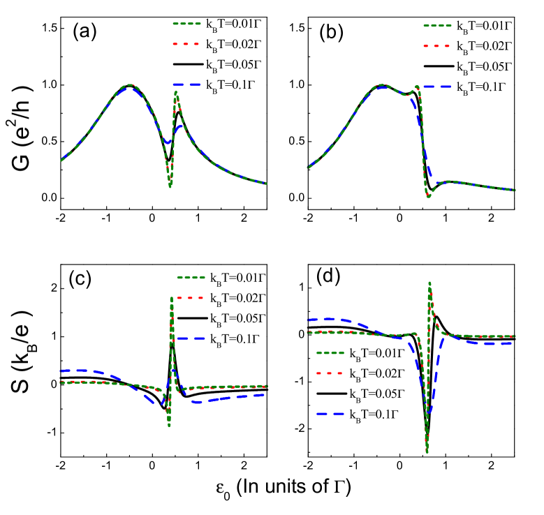
Figure 2: (a) and (b), the electronic conductances with the increase of temperature, in the cases of $\phi=0$ and $\phi=\pi$, respectively. And, the corresponding thermopowers are shown in (c) and (d).

III Numerical results and discussions

With the formulation developed in the above section, we perform the numerical calculation to investigate the thermoelectric properties of the parallel double-QD structure. Prior to the calculation, we need to introduce a parameter $\Gamma$ as the unit of energy.

According to the discussions in the previous work, this structure is usually used to research the well-known Fano effect of QD system by adjusting its arms as nonresonant and resonant channels for electron transmission. Based on such a result, we here would like to focus on the thermoelectric effect influenced by the Fano interference in the parallel double-QD structure. First, we choose $\Gamma_{22}=10\Gamma_{11}=\Gamma$ to achieve the nonresonant and resonant transport for the Fano interference. With respect to the QD levels, we take $\varepsilon_{1}=\varepsilon_{0}-{\Gamma\over 2}$ and $\varepsilon_{2}=\varepsilon_{0}+{\Gamma\over 2}$, respectively. In experiment, $\varepsilon_{0}$ can be changed with respect to the zero point energy via adjusting the gate voltage. Surely, $\varepsilon_{1}$ and $\varepsilon_{2}$ can be viewed as the levels of the bonding and antibonding states of the coupled double QDs. In Fig.2, we plot the spectra of electronic conductance and thermopower as functions of $\varepsilon_{0}$ (i.e., the QD level), respectively. Fig.2(a) shows the spectra of the electronic conductance vs $\varepsilon_{0}$ in the absence of magnetic field. We observe that at low temperature, e.g., $k_{B}T\leq 0.02\Gamma$, the electronic conductance spectrum shows up as a Fano lineshape. With the increase of temperature, the Fano lineshape in the electronic conductance spectrum becomes ambiguous. We can understand that such a result arises from the destructive effect of the increase of temperature on the Fano interference here. Next, in Fig.2(b) we see that the Fano lineshape in the conductance spectrum is reversed in the case of a magnetic flux through the ring with $\phi=\pi$. Also, with the increase of temperature the Fano lineshape becomes unclear. However, from Fig.2(a)-(b), we observe that in the two cases that $\phi=0$ and $\phi=\pi$, temperature plays different roles in modifying the Fano interference. To be precise, in the zero-magnetic-flux case, the conductance lineshape is destroyed more seriously by the increase of temperature. When $k_{B}T=0.05\Gamma$, the Fano dip in the conductance spectrum is significantly raised, accompanied by the suppression of the Fano peak. But, in the case of $\phi=\pi$, the conductance spectrum is weakly dependent on the increase of temperature, so that the Fano lineshape can still be seen in the conductance spectrum in the case that $k_{B}T=0.05\Gamma$.

In Fig.2(c)-(d), we investigate the Seebeck effect in the cases of $\phi=0$ and $\pi$, respectively. From the two figures, we see that the nonzero Seebeck coefficient only appears in the energy region where the Fano interference occurs (Hereafter we call such a region the “Fano region” for simplicity). Hence, it is evident that in this structure the Seebeck effect is closely dependent on the Fano interference. Consequently, at low temperature when the Fano interference is strong, the magnitude of Seebeck coefficient is large. And, the increase of temperature weakens the Fano interference, so that the magnitude of Seebeck coefficient becomes small. Also due to such a reason, the different Fano lineshapes, i.e., the different Fano interferences in these two cases cause two different results about the Seebeck effects. To be specific, in the zero-magnetic-flux case, the value of Seebeck coefficient is greater than zero in the Fano region. But when the magnetic flux is applied with $\phi=\pi$, the sign of the Seebeck coefficient becomes negative. In addition, it shows that in the case of zero magnetic field, the magnitude of the Seebeck coefficient is suppressed with the increase of temperature. Especially when $k_{B}T=0.1\Gamma$, the magnitude of $S$ is almost less than $0.5$. However, at the case of $\phi=\pi$, the temperature dependence of $S$ is weak. Accordingly, we obtain the result that $S\approx 2$ when $k_{B}T=0.1\Gamma$.

It should be pointed out that the different thermoelectric properties in the cases of $\phi=0$ and $\phi=\pi$ originate from the different Fano interference mechanisms. Next, we try to clarify the difference between the Fano interferences in such two cases by employing the concept of Feynman path. With this idea, we rewrite the electron transmission function as $T(\omega)=4\mathrm{Tr}[\Gamma^{L}G^{r}\Gamma^{R}G^{a}]=|\sum\limits_{j,n=1}^{2}t(j,n)|^{2}$. Herein, the electron transmission coefficients are defined as $t(j,n)=\bar{V}_{{\scriptscriptstyle L}j}G^{r}_{jn}\bar{V}_{n{\scriptscriptstyle R}}$ with $\bar{V}_{j\alpha}=\bar{V}_{\alpha j}^{*}=V_{j\alpha}\sqrt{2\pi\rho_{\alpha}(\omega)}$. Then, we expand the Green function into an infinite geometric series, e.g., $G^{r}_{11}=\frac{g^{-1}_{2}}{g^{-1}_{1}g^{-1}_{2}+\Gamma_{12}\Gamma_{21}}=\sum\limits_{j=0}^{\infty}g_{1}(-g_{1}g_{2}\Gamma_{12}\Gamma_{21})^{j}$. Following the expansion of the Green function, the transmission coefficient $t(1,1)$ can be expressed as a summation of Feynman paths with different orders, i.e.,

$$t(1,1)=\sum\limits_{j=0}^{\infty}\bar{V}_{{\scriptscriptstyle L}1}g_{1}(-g_{1}g_{2}\Gamma_{12}\Gamma_{21})^{j}\bar{V}_{1{\scriptscriptstyle R}}=\sum\limits_{j=0}^{\infty}t_{j}(1,1).$$ (17)

For example, $t_{0}(1,1)=\bar{V}_{{\scriptscriptstyle L}1}g_{1}\bar{V}_{1{\scriptscriptstyle R}}$ is the zero-order Feynman path from lead-$L$ to lead-$R$ via QD-1. For the first-order Feynman path, it can be written as $t_{1}(1,1)=-\bar{V}_{{\scriptscriptstyle L}1}g^{2}_{1}g_{2}\Gamma_{12}\Gamma_{21}\bar{V}_{1{\scriptscriptstyle R}}$, which consists of four terms representing individual Feynman paths. They are denoted as

$$\left\{\begin{array}[]{cccc}t_{1a}(1,1)&=&-\bar{V}_{{\scriptscriptstyle L}1}g_{1}\widetilde{V}_{1{\scriptscriptstyle L}}\widetilde{V}_{{\scriptscriptstyle L}2}g_{2}\widetilde{V}_{2{\scriptscriptstyle L}}\widetilde{V}_{{\scriptscriptstyle L}1}g_{1}\bar{V}_{1{\scriptscriptstyle R}},\\ t_{1b}(1,1)&=&-\bar{V}_{{\scriptscriptstyle L}1}g_{1}\widetilde{V}_{1{\scriptscriptstyle L}}\widetilde{V}_{{\scriptscriptstyle L}2}g_{2}\widetilde{V}_{2{\scriptscriptstyle R}}\widetilde{V}_{{\scriptscriptstyle R}1}g_{1}\bar{V}_{1{\scriptscriptstyle R}},\\ t_{1c}(1,1)&=&-\bar{V}_{{\scriptscriptstyle L}1}g_{1}\widetilde{V}_{1{\scriptscriptstyle R}}\widetilde{V}_{{\scriptscriptstyle R}2}g_{2}\widetilde{V}_{2{\scriptscriptstyle L}}\widetilde{V}_{{\scriptscriptstyle L}1}g_{1}\bar{V}_{1{\scriptscriptstyle R}},\\ t_{1d}(1,1)&=&-\bar{V}_{{\scriptscriptstyle L}1}g_{1}\widetilde{V}_{1{\scriptscriptstyle R}}\widetilde{V}_{{\scriptscriptstyle R}2}g_{2}\widetilde{V}_{2{\scriptscriptstyle R}}\widetilde{V}_{{\scriptscriptstyle R}1}g_{1}\bar{V}_{1{\scriptscriptstyle R}},\end{array}\right.$$ (18)

with $\widetilde{V}_{j\alpha}=\widetilde{V}_{\alpha j}^{*}=V_{j\alpha}\sqrt{\pi\rho_{\alpha}(\omega)}$.

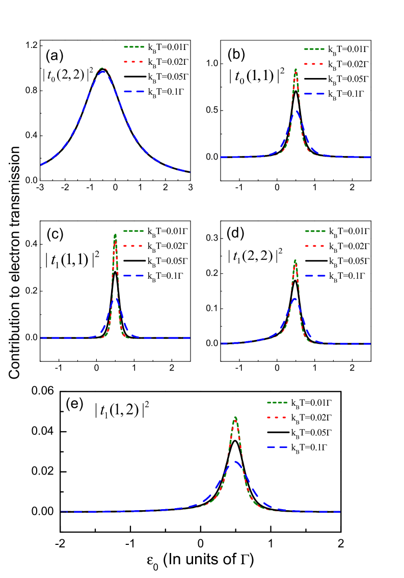
Figure 3: The contributions of the zero- and first-order Feynman paths to the electron transmission at the case of zero magnetic field.

Similarly, we can expand other transmission coefficients as a summation of Feynman paths, e.g.,

$$t(1,2) = \sum\limits_{j=1}^{\infty}i\bar{V}_{{\scriptscriptstyle L}1}(-g_{1}g_{2}\Gamma_{12})^{j}\Gamma_{21}^{j-1}\bar{V}_{2{\scriptscriptstyle R}}=\sum\limits_{j=1}^{\infty}t_{j}(1,2).$$

The lowest-order Feynman paths of $t(1,2)$ can be written as

$$\left\{\begin{array}[]{ccc}t_{1a}(1,2)&=&-i\bar{V}_{{\scriptscriptstyle L}1}g_{1}\widetilde{V}_{1{\scriptscriptstyle L}}\widetilde{V}_{{\scriptscriptstyle L}2}g_{2}\bar{V}_{2{\scriptscriptstyle R}},\\ t_{1b}(1,2)&=&-i\bar{V}_{{\scriptscriptstyle L}1}g_{1}\widetilde{V}_{1{\scriptscriptstyle R}}\widetilde{V}_{{\scriptscriptstyle R}2}g_{2}\bar{V}_{2{\scriptscriptstyle R}}.\end{array}\right.$$ (20)

By the same approach, the Feynman paths arising from $t(2,2)$ and $t(2,1)$ can be clarified.

Via the analysis above, we can clearly know that the Fano effect in this structure originates from the quantum interference among infinite Feynman paths. But when the magnetic flux is introduced with $\phi=\pi$, the contribution of the higher-order Feynman paths will vanish due to the destructive interference among them. Then in such a case, the two QDs become decoupled from each other with $\Gamma_{jn}=0$ $(j\neq n)$. And, the interference between $t_{0}(1,1)$ and $t_{0}(2,2)$ leads to the Fano effect. Based on this viewpoint, we can understand that the different Fano lineshapes in the electronic conductance spectra arise from the dissimilar Fano interference mechanisms. Also for such a reason, the thermoelectric effect in these two cases present different properties. With the help of the Feynman path method, we next illustrate the sensitive effect of temperature in the case of $\phi=0$. In Fig.3, we investigate the contributions of the zero- and first-order Feynman paths to the electronic conductance. For the zero-order paths, we find that the increase of temperature can not affect the magnitude of $t_{0}(2,2)$, whereas the resonant path $t_{0}(1,1)$ is destroyed via the increase of temperature. Surely, such a result brings about the temperature-induced change of Fano effect in the case of $\phi=\pi$. Next, in Fig.3(c)-(e) one sees that by the increase of temperature, the contributions of the first-order paths are weakened seriously. This is because that the temperature increase destroys the coherent transmission in the paths. According to this result, we can ascertain that the contributions of the higher-order paths will decrease seriously with the increase of temperature, since the complication of high-order paths. Thus, even if the same increase of temperature, the quantum interference of $\phi=0$ will be further weakened, compared with the case of $\phi=\pi$. Up to now, we have understood the sensitive effect of temperature on decrease of thermoelectric efficiency in the zero-magnetic-flux case.

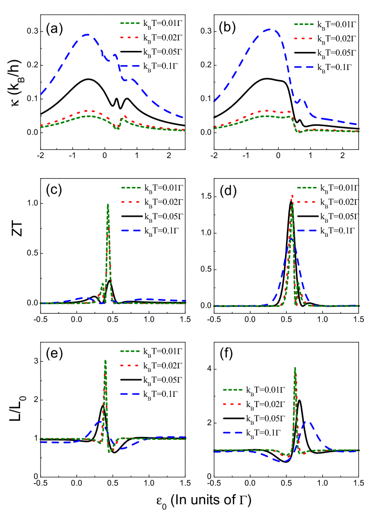
Figure 4: (a) and (b) The thermal conductances affected by the temperature increase, in the cases of $\phi=0$ and $\phi=\pi$, respectively. The corresponding thermal efficiencies are respectively shown in (c) and (d), whereas the Lorenz numbers are in (e) and (f).

In the following, we investigate the thermal conductance $\kappa$, figure of merit $ZT$, and Lorenz number $L$ in this structure, respectively. The numerical results are shown in Fig.4. First, in Fig.4(a)-(b) we show the thermal conductance spectra in the cases of $\phi=0$ and $\phi=\pi$, respectively. In these two figures, we observe that only at low temperature (e.g., $k_{B}T\leq 0.02\Gamma$), the thermal conductance spectra are similar to those of electronic conductance. But, the temperature dependence of thermal conductance is more sensitive compared with the electronic conductance, especially in the case of zero magnetic flux. Typically, when temperature increases to $k_{B}T=0.05\Gamma$, the value of thermal conductance is raised and a sub-peak emerges in the Fano region of the thermal conductance spectrum. Alternatively, for the case of $\phi=\pi$, in the Fano region the thermal conductance increases a little with the increase of temperature to $k_{B}T=0.05\Gamma$. Next, Fig.4(c)-(d) show the spectra of figure of merit $ZT$ with the change of QD level. Here we see that in the zero-magnetic-flux case, the magnitude of $ZT$ is always less than one. And, with the increase of temperature, the value of $ZT$ decreases to a large degree. For instance, in the case of $k_{B}T=0.1\Gamma$, the value of $ZT$ is almost close to zero. But when $\phi=\pi$, the thermoelectric efficiency is enhanced to a large degree in the Fano region. Even if $k_{B}T=0.1\Gamma$, the magnitude of $ZT$ is close to one. Besides, we see that in such a case, the figure of merit is nearly independent of the increase of temperature at low temperature of $k_{B}T\leq 0.05\Gamma$. Now, we can clarify the difference of the thermoelectric properties in these two cases.

It is known that in the bulk materials the thermal and electric conductances at low temperature are related by the Wiedemann-Franz law, i.e., $\kappa/{\cal G}T=L_{0}$, where $L_{0}=k_{B}^{2}\pi^{3}/3e^{2}$. Then, in order to investigate the violation of Wiedemann-Franz law in such a structure, we reassume $L=\kappa/{\cal G}T$ and evaluate the value of $L/L_{0}$ in Fig.4(e)-(f). It is seen that in both cases of $\phi=0$ and $\phi=\pi$, the Lorenz number is deviated from its classical value in the Fano region. And, at the same temperature, the value of $L/L_{0}$ in the case of $\phi=\pi$ is much larger than that in the case of $\phi=0$. In addition, it is obvious that with the increment of temperature, the magnitude of $L/L_{0}$ decreases since the weakness of the Fano interference effect.

We readily find that all the configurations of coupled double QDs can be mapped into the above model by means of representation transformation. So, the thermoelectric properties of the above model can help to further understand those of coupled double-QD systems. On the other hand, in order to clarify the thermoelectric properties of coupled double QDs, it is necessary for us to transform its QD Hamiltonian into the molecular orbital representation. We take the parallel coupled double QDs as an example to illustrate such an issue. The single-electron Hamiltonian of it is given by $h=\underset{k,\alpha\in L,R}{\sum}\varepsilon_{\alpha k}c_{\alpha k}^{\dagger}c_{\alpha k}+\sum_{j=1}^{2}e_{j}f_{j}^{\dagger}f_{j}+\lambda f^{\dagger}_{1}f_{2}+\underset{\alpha kj}{\sum}w_{j\alpha}f_{j}^{\dagger}c_{\alpha k}+{\mathrm{h.c.}}$. $f^{{\dagger}}_{j\sigma}$ $(f_{j\sigma})$ is the creation (annihilation) operator of electron in QD-$j$. $e_{j}$ denotes the electron level in the corresponding QD. $\lambda$ is the interdot coupling. $w_{j\alpha}$ denotes the coupling between the QDs and leads, which is real in the absence of magnetic flux. As reported by the some works, such a structure possesses interesting thermoelectric properties.Trocha Let us analyze this structure by mapping the QD Hamiltonian into its molecular orbital representation. We obtain the relation between QD level $e_{j}$ and eigenlevel $\varepsilon_{j}$, i.e., $\varepsilon_{1}=\frac{1}{2}\bigg{(}e_{1}+e_{2}-\sqrt{(e_{1}-e_{2})^{2}+4\lambda^{2}}\bigg{)}$ and $\varepsilon_{2}=\frac{1}{2}\bigg{(}e_{1}+e_{2}+\sqrt{(e_{1}-e_{2})^{2}+4\lambda^{2}}\bigg{)}$. Besides, the couplings between the molecular states and lead-$\alpha$ are expressed as $\left[\begin{array}[]{ccc}V_{1\alpha}\\ V_{2\alpha}\end{array}\right]=[\bm{\eta}]\left[\begin{array}[]{ccc}w_{1\alpha}\\ w_{2\alpha}\end{array}\right]$ with

$$[\bm{\eta}]=\left[\begin{array}[]{ccc}\sqrt{\frac{\lambda^{2}}{\lambda^{2}+(\varepsilon_{1}-e_{1})^{2}}}&\sqrt{\frac{(\varepsilon_{1}-e_{1})^{2}}{\lambda^{2}+(\varepsilon_{1}-e_{1})^{2}}}\\ -\sqrt{\frac{\lambda^{2}}{\lambda^{2}+(\varepsilon_{2}-e_{1})^{2}}}&\sqrt{\frac{(\varepsilon_{2}-e_{1})^{2}}{\lambda^{2}+(\varepsilon_{2}-e_{1})^{2}}}\end{array}\right].$$

With the above results, the coupling strengths between the molecular states and the leads can be evaluated, i.e., $\Gamma^{\alpha}_{jj}=\pi|\eta_{j1}w_{1\alpha}+\eta_{j2}w_{2\alpha}|^{2}\rho_{\alpha}(\omega)$ and $\Gamma^{\alpha}_{jl}=\pi(\eta_{j1}w_{1\alpha}+\eta_{j2}w_{2\alpha})(\eta^{*}_{n1}w^{*}_{1\alpha}+\eta^{*}_{n2}w^{*}_{2\alpha})\rho_{\alpha}(\omega)$. It is certain that the couplings between the molecular states and the leads determine the quantum transport properties of coupled double QDs. When changing $e_{j}$ and $w_{j\alpha}$ to satisfy the condition of $\Gamma_{jj}\ll\Gamma_{nn}$, we achieve the resonant and nonresonant channels for electron transmission, so that the Fano effect will occur. One will then observe the enhancement of thermoelectric efficiency. Such a result can be attributed to the destructive quantum interference among infinite Feynman paths. Moreover, for a typical structure with $e_{j}=\varepsilon_{0}$, $\lambda={\Gamma\over 2}$, and $|w_{j\alpha}|=2|w_{n\alpha}|$, there will be $\Gamma_{jj}\approx 10\Gamma_{nn}$. Then, in the configuration of left-right symmetry, i.e., $w_{jL}=w_{jR}$, the quantum interference and the thermoelectric behaviors just correspond to the case of $\phi=0$ in our model. Alternatively, for a structure with $w_{jL}=w_{nR}$, there will be $\Gamma_{jn}=0$ ($j\neq n$). The thermoelectric properties will be the same as those in our model of $\phi=\pi$, which is caused by the Fano interference which occurs between two zero-order Feynman paths. Up to now, by analyzing the quantum interference of the coupled double-QD structure, we have clarified its thermoelectric features.

At last, we would like to state that the theory in this work can be generalized to discuss the thermoelectric effect of the multi-QD structures. From the previous literature,Orellana ; jpcm ; pap we know that multi-QD systems possess abundant quantum interference mechanism. And in such systems, the couplings between some molecular states and leads act as nonresonant channels while the states provide resonant channels for electron transmission, so the Fano effect comes into being. Besides, since so many tunable structure parameters, in multi-QD systems the Fano effect is more intricate compared with double-QD structures. Therefore, we are sure that the thermoelectric properties of these structures are of much interest. With the help of our analysis, we here readily discuss the thermoelectric results of multi-QD structure modulated by the Fano effect. By mapping the QD Hamiltonian into its molecular orbital representation, we can first clarify the feature of Fano effect. In the case of $\Gamma_{jn}\neq 0$ ($j\neq n$), the Fano effect arises from the quantum interference among infinite Feynman paths. And in such a case, thermoelectric quantities are more sensitive to the change of temperature, compared with the structure of double QDs. This is because that in multi-QD structures, the Feynman paths become more complicated. But when the coupling manners between the molecular states are $\Gamma_{jn}=0$ ($j\neq n$), it is certain that the Fano effect is caused by the quantum interference among the zero-order Feynman paths. Then, similar to the double-QD structure, the temperature dependence of the thermoelectric quantities is relatively weak. Therefore, the analysis about the thermoelectric properties of the double QDs can be generalized to multi-QD case. Therefore, we believe that our work is helpful for the understanding about the thermoelectric properties of coupled-QD systems which are induced by the Fano effect.

IV summary

To sum up, in this paper we have discussed the thermoelectric properties assisted by the Fano effect in a parallel double QD structure. By adjusting the the couplings between the QDs and leads, we facilitated the nonresonant and resonant channels for the Fano interference. It was found that at low temperature, Fano lineshapes appear in the electronic and thermal conductance spectra. And, the Fano lineshapes can be reversed by applying a local magnetic flux with the magnetic phase factor $\phi=\pi$. It showed that the Fano effect contributes nontrivially to the enhancement of the thermoelectric efficiency. Furthermore, in the cases of $\phi=0$ and $\phi=\pi$, the different-property Fano interferences induced the different thermoelectric effects. Namely, by the presence of magnetic flux with $\phi=\pi$, the thermoelectric effect is much more apparent compared with that in the zero-magnetic-flux case. By employing the concept of Feynman path, the physics reason was clarified. To be concrete, the Fano effect of $\phi=0$ is caused by the quantum interference among infinite Feynman paths. Hence, it is sensitive to the temperature increase, since the increase of temperature can effectively suppress the coherent transmission in each path. In contrast, the Fano interference of $\phi=\pi$, resulting from the interference between two zero-order paths, is less dependent on the temperature increase. Next, at the end of the text, we discussed the feasibility of our theory in multi-QD structures. We hope that the theory of this work is helpful for understanding the thermoelectric properties contributed by the Fano effect of coupled-QD systems.

References

- (1) F. Giazotto, T. T. Heikkilā, A. Luukanen, A. M. Savin, and J. P. Pekola, Rev. Mod. Phys. 78, 217 (2006).
- (2) M. F. Ódwyer, R. A. Lewis, C. Zhang, and T. E. Humphrey, Phys. Rev. B 72, 205330 (2005).
- (3) M. S. Dresselhaus, G. Chen, M. Y. Tang, R. G. Yang, H. Lee, D. Z. Wang, Z. F. Ren, J.-P. Fleurial, and P. Gogna, Adv. Mater. 19, 1043 (2007).
- (4) G. Mahan, B. Sales, and J. Sharp, Phys. Today 50, 42 (1997).
- (5) G. Grosso and G. P. Parravicini, Solid State Physics (Academic Press, Amsterdam 2000).
- (6) A. Majumdar, Science 303, 777 (2004).
- (7) T. C. Harman, P. J. Taylor, M. P. Walsh, and B. E. LaForge, Science 297, 2229 (2002).
- (8) R. Venkatasubramanian, E. Siivola, T. Colpitts, and B. ÓQuinn, Nature 413, 597, (2001).
- (9) K. F. Hsu, S. Loo, F. Guo, W. Chen, J. S. Dyck, C. Uher, T. Hogan, E. K. Polychroniadis, and M. G. Kanatzidis, Science 303, 818 (2004).
- (10) B. Poudel, Q. Hao, Y. Ma, Y. Lan, A. Minnich, B. Yu, X. Yan, D. Wang, A. Muto, D. Vashaee, X. Chen, J. Liu, S. Dresselhaus, M. G. Chen, and Z. Ren, Science 320, 634 (2008).
- (11) A. I. Hochbaum, R. Chen, R. D. Delgado, W. Liang, E. C. Garnett, M. Najarian, A. Majumdar, and P. Yang, Nature 451, 163 (2008).
- (12) A. I. Boukai, Y. Bunimovich, J. Tahir-Kheli, J.-K. Yu, W. A. Goddard III, and J. R. Heath Nature 451, 168 (2008).
- (13) H.-K. Lyeo, A. A. Khajetoorians, L. Shi, K. P. Pipe, R. J. Ram, A. Shakouri, and C. K. Shih, Science 303, 816 (2004).
- (14) L. D. Hicks and M. S. Dresselhaus, Phys. Rev. B 47, 12727 (1993); ibid. Phys. Rev. B 47, 16631 (1993).
- (15) A. Khitun, A. Balandin, J. L. Liu, and K. L. Wang, J. Appl. Phys. 88, 696 (2000).
- (16) R. Fletcher, E. Zaremba and U. Zeitler, Electron-Phonon Interactions in Low Dimensional Structures ed. L. Challis (Oxford: Oxford University Press 2003) p149.
- (17) M. Tsaousidou, The Oxford Handbook of Nanoscience and Technology vol II, ed. A. V. Narlikar and Y. Y. Fu (Oxford: Oxford University Press 2010) chapter 13, p477.
- (18) G. D. Mahan and J. O. Sofo, Proc. Natl Acad. Sci. USA 93, 7436 (1996); M. Paulsson and S. Datta, Phys. Rev. B 67, 241403(R) (2003).
- (19) M. Tsaousidou and G.P. Triberis, J. Phys.: Condens. Matter 22, 355304 (2010).
- (20) R. Świrkowicz, M. Wierzbicki, and J. Barnaś, Phys. Rev. B 80, 195409 (2009).
- (21) C. W. J Beenakker and A. A. M. Staring, Phys. Rev. B 46, 9667 (1992).
- (22) Y. M. Blanter, C. Bruder, R. Fazio, and H. Schoeller, Phys. Rev. B 55, 4069 (1997); M. Turek and K. A. Matveev, Phys. Rev. B 65, 115332 (2002).
- (23) J. Koch, F. von Oppen, Y. Oreg, and E. Sela, Phys. Rev. B 70, 195107 (2004).
- (24) B. Kubala and J. Konig, Phys. Rev. B 73, 195316 (2006); B. Kubala, J. Konig, and J. Pekola, Phys. Rev. Lett. 100, 066801 (2008).
- (25) X. Zianni, Phys. Rev. B 75, 045344 (2007).
- (26) R.-Q. Wang, L. Sheng, R. Shen, B. Wang, and D. Y. Xing, Phys. Rev. Lett. 105, 057202 (2010).
- (27) J. Liu, Qing-feng Sun, X. C. Xie, Phys. Rev. B 81, 245323 (2010).
- (28) D. Boese and R. Fazio, Europhys. Lett. 56, 576 (2001).
- (29) B. Dong and X. L. Lei, J. Phys.: Condens. Matter 14, 11747 (2002).
- (30) M. Krawiec and K. I. Wysokiński, Phys. Rev. B 73, 075307 (2006).
- (31) R. Sakano, T. Kita, and N. Kawakami, J. Phys. Soc. Jpn. 76, 074709 (2007).
- (32) R. Scheibner, H. Buchmann, D. Reuter, M. N. Kiselev, and L. W. Molenkamp, Phys. Rev. Lett. 95, 176602 (2005).
- (33) M. Yoshida and L. N. Oliveira, Physica B 404, 3312 (2009).
- (34) T. K. T. Nguyen, M. N. Kiselev, and V. E. Kravtsov, Phys. Rev. B 82, 113306 (2010)
- (35) T.A. Costi and V. Zlatic, Phys. Rev. B 81, 235127 (2010).
- (36) P. Murphy, S. Mukerjee, and J. Moore, Phys. Rev. B 78, 161406 (2008).
- (37) David M.-T. Kuo and Yia-Chung Chang, Phys. Rev. Lett. 95, 066801 (2005); G. A. Lara, P. A. Orellana, and E. V. Anda, Phys. Rev. B 78, 045323 (2008); B. Dong and X. L. Lei, and N. J. M. Horing, Phys. Rev. B 77, 085309 (2008).
- (38) F. Qassemi, W. A. Coish, and F. K. Wilhelm, Phys. Rev. Lett. 102, 176806 (2009); A. B. Vorontsov and M. G. Vavilov, Phys. Rev. Lett. 101, 226805 (2008).
- (39) R. Leturcq, L. Schmid, K. Ensslin, Y. Meir, D. C. Driscoll, and A. C. Gossard, Phys. Rev. Lett. 95, 126603 (2005); T. Kuzmenko, K. Kikoin, and Y. Avishai, Phys. Rev. Lett. 96, 046601 (2006); J. C. Chen, A. M. Chang, and M. R. Melloch, Phys. Rev. Lett. 92, 176801 (2004).
- (40) K.-W. Chen and C.-R. Chang, Phys. Rev. B 78, 235319 (2008); Z. Jiang and Q.-Z. Han, Phys. Rev. B 78, 035307 (2008).
- (41) K. Bao and Y. Zheng, Phys. Rev. B 73, 045306 (2005).
- (42) X. Chen, H. Buhmann, and L. W. Molenkamp, Phys. Rev. B 61, 16801 (2000).
- (43) C. M. Finch, V. M. García-Suárez and C. J. Lambert, Phys. Rev. B 79, 033405 (2009).
- (44) M. Wierzbicki and R. Swirkowicz, Phys. Rev. B 84, 075410 (2011).
- (45) D. M.-T. Kuo and Yia-chung Chang, arXiv:1104.2651v3.
- (46) F. Pauly, J. K. Viljas, and J. C. Cuevas, Phys. Rev. B 78, 035315 (2008).
- (47) Y. S. Liu and X. F. Yang, J. Appl. Phys. 108, 023710 (2010).
- (48) O. Karlström, H. Linke, G. Karlström, and A. Wacker, arXiv: 1107.0572v1.
- (49) Piotr Trocha and J. Barnaś, arXiv: 1108.2422v1.
- (50) U. Fano, Phys. Rev. 124, 1866 (1961).
- (51) M. Sato, H. Aikawa, K. Kobayashi, S. Katsumoto, and Y. Iye, Phys. Rev. Lett. 95, 066801 (2005); K. Kobayashi, H. Aikawa, A. Sano, S. Katsumoto, and Y. Iye, Phys. Rev. B 70, 035319 (2003).
- (52) B. Kubala and J. König, Phys. Rev. B 65, 245301 (2002).
- (53) Y. Meir and N. S. Wingreen, Phys. Rev. Lett. 68, 2512 (1992); A. P. Jauho, N. S. Wingreen, and Y. Meir, Phys. Rev. B 50, 5528 (1994).
- (54) T.-S. Kim and S. Hershfield, Phys. Rev. Lett. 88, 136601 (2002); Phy. Rev. B 67, 165313 (2003).
- (55) W. Gong, Y. Zheng, Y. Liu, and T. Lu, Physica E 40, 618(2008).
- (56) M. L. Ladrón de Guevara and P. A. Orellana, Phys. Rev. B 73, 205303 (2006).
- (57) W. Gong, Y. Han, and G. Wei, J. Phys.: Condens. Matter 21, 175801 (2009).
- (58) W. Gong and C. Jiang, J. Appl. Phys. 106, 013710 (2009).