Thermodynamics of localized magnetic moments in a Dirac conductor

Abstract

We show that the magnetic susceptibility of a dilute ensemble of magnetic impurities in a conductor with a relativistic electronic spectrum is non-analytic in the inverse tempertature at $T^{-1}\to 0$. We derive a general theory of this effect and construct the high-temperature expansion for the disorder averaged susceptibility to any order, convergent at all tempertaures down to a possible ordering transition. When applied to Ising impurities on a surface of a topological insulator, the proposed general theory agrees with Monte Carlo simulations, and it allows us to find the critical temperature of the ferromagnetic phase transition.

Collective phenomena in random ensembles of magnetic impurities embedded in metallic conductors are caused by the long-distance exchange interaction mediated by the mobile carriers, also known as the RKKY exchange RKKY . The RKKY interaction has a well studied universal structure for all metallic systems RKKYClass , with the exception of the recently discovered class of two dimensional (2D) materials in which the low-energy electron excitations resemble massless Dirac particles: graphene GrapheneDiscovery ; Castro , chiral metals formed at the surface of topological insulators ChiralMetal ; ChiralMetal1 , and silicene silicene . Recent experiments Chen and Wray have reported the formation of a band gap in a chiral metal contaminated by magnetic impurities, pointing towards magnetic ordering at the surface of the topological insulator; also theoretical modelling suggested ordering transition in some of such systems Structural ; Abanin .

There are two peculiarities of the RKKY exchange in conductors with the Dirac-like electron spectrum which make it qualitatively different from usual metals: (i) the exchange interaction as a function of distance between two impurities shows the unusual $1/r^{3}$ decay law, (ii) the Friedel oscillations are either absent or comensurate with the lattice Graphene-Friedel . In the following, we shall call such interaction a Dirac-RKKY exchange. Other details of the RKKY exchange such as its anisotropy or whether it is ferromagnetic, antiferromagnetic or depolarizing may depend on the material and the symmetry of the impurity position in the lattice. In this Letter we propose a general quantitative theory of the thermodynamics of an ensemble of randomly positioned magnetic impurities interacting through the Dirac-RKKY exchange in a paramagnetic phase, that is at temperatures above the magnetic ordering temperature $T_{c}.$ We show that, due to a peculiar decay law of the Dirac-RKKY exchange, the magnetic susceptibility shows a strong deviation from the Curie-Weiss law seen as non-analiticity in its high-temperature expansion,

$$\chi=\frac{c_{0}}{T}\sum_{n=1}^{\infty}C_{n}\left(\frac{T_{0}}{T}\right)^{\frac{2}{3}(n-1)},$$ (1)

where $c_{0}$ is the Curie constant, $s$ is the impurity spin quantum number, $T_{0}\propto\rho^{3/2}$ is a temperature scale dependent on the density of impurities, $\rho,$ and $C_{n}$ are numerical coefficients expressed in terms of finite-dimensional integrals of elementary functions, see Eqs. (9), (10). The expansion (1) also encodes detailed information about the critical point of a magnetic transition: the value of $T_{c}$ and the susceptibility critical exponent $\gamma$ can be extracted from the values of several coefficients $C_{n}$ with the help of Padé approximation Baker1975 . One example of a successful application of the proposed theory is illustrated in Fig. 1, where the susceptibility obtained with the help of Eq. (1) is compared with the Monte Carlo data for the archetypal Dirac-RKKY system of randomly positioned Ising spins with ferromagnetic $1/r^{3}$ exchange. Numerical values of the coefficient $C_{2}$ for some other Dirac-RKKY models are presented in Table 1.

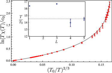
Figure 1: Magnetic susceptibility of the Dirac-RKKY Ising model. The solid line shows the L=5 D-log Padé approximant calculated from the first twelve terms in the expansion (1) (see Table 2 for the numerical values of the coefficients $C_{n}$). The points with error bars are the results of the Monte Carlo simulation. The error bars show the statistical uncertainty arising from both MC fluctuations and quenched disorder. Inset: The approximate critical temperature derived from the position of the singularity of the D-log Padé approximant. The error bars show the uncertainty due to the finite precision of the expansion coefficients in Table 2. The thin dotted line shows the best aproximation for the critical temperature.

A pair of localized spins separated by a distance exceeding a few lattice constants experiences the RKKY interaction mediated by electrons near the Fermi surface, which in Dirac conductors consists of a discrete set of points in the reciprocal space. In graphene there are two Fermi points related by time reversal symmetryCastro . In topological insulators where the ultrarelativistic electrons reside at the surface, there may be one Fermi point per face ChiralMetal . The dispersion relation of the electronic excitations near each Fermi point is $\epsilon(p)=\pm\hbar vp,$ where $p$ is the Bloch wave number of an electron relative to the Fermi point. Due to the discrete geometry of the Fermi sufrace and the linear dispersion of the excitations, the Dirac-RKKY interaction does not exhibit Friedel oscillations found in usual metals and decays as $1/r^{3}$ as a function of distance $r$ between spins Structural ; Graphene-RKKY . This decay law is valid in a broad range of lengths $r_{E}<r<r_{T},$ where $r_{E}=\hbar v/E$ is the length scale associated with the binding energy $E$ ($\sim 1$ eV) of adatom, and $r_{T}=\hbar v/kT$ is the thermal wevelength of an electron. The most general form of the Dirac-RKKY Hamiltonian of a system of $N$ impurities in a magnetic field is

$$H_{12\dots N}=J\sum_{i<j}^{N}\frac{G_{ij}}{r_{ij}^{3}}-hS_{z}\ ,$$ (2)

$$G_{ij}=G(\mathbf{s}_{i},\mathbf{s}_{j},\mathbf{n}_{ij},\xi_{i},\xi_{j}).$$

Here the sum is taken over all pairs of impurities randomly distributed with the average density $\rho$ in the conductor plane, and $r_{ij}=|\mathbf{r}_{i}-\mathbf{r}_{j}|$ is the distance between a pair of adatoms with quenched positions $\mathbf{r}_{i}$ and $\mathbf{r}_{j}.$ In Eq. (2) we assume without loss of generality that the magnetic field $h$ is coupled to the $z$-projection of the total spin $S_{z}=s_{1}^{z}+\dots s_{N}^{z},$ and the spin of each impurity is assumed to be in the $2s+1$ dimensional representation of SU(2). The parameter $J$ is specific for the given host material and the type of impurity. Together with the impurity density $\rho$ it defines the energy scale

$$T_{0}=\frac{s(s+1)J}{3}\rho^{3/2}.$$ (3)

Further material-dependent details of the RKKY interaction are encoded in the dimensionless pairwise interaction function $G_{ij},$ which depends on two impurity spins $\mathbf{s}_{i},\mathbf{s}_{j},$ a unit vector $\mathbf{n}_{ij}=\mathbf{r}_{ij}/r_{ij}$ and two discrete quenched random variables $\xi_{i},\xi_{j}$ defining the position of each adatom inside the lattice unit cell Structural ; footnote1 (see Table 1 for examples).

Dirac-RKKY ensemble	$G_{ij}$	Observable	$C_{2}$	$\Theta/T_{0}$
Spin 1/2 Ising impurities.	$-s_{i}^{z}s_{j}^{z}$	$S_{z}$	$9.02$	$27.1$
Spin 1/2 impurities isotropically coupled to the electrons in a chiral metal.	$-s_{i}^{z}s_{j}^{z}-(\mathbf{n}\cdot\mathbf{s}_{i})(\mathbf{n}\cdot\mathbf{s}_{j})+\frac{1}{2}(\mathbf{n}\times\mathbf{s}_{i})_{z}(\mathbf{n}\times\mathbf{s}_{j})_{z}$	$S_{z}$	$9.59$	$29.7$
		$S_{x}$	$1.18$	$1.28$
Spin 1/2 impurities with X-Y coupling to the electrons in a chiral metal.	$-(\mathbf{n}\cdot\mathbf{s}_{i})(\mathbf{n}\cdot\mathbf{s}_{j})+\frac{1}{2}(\mathbf{n}\times\mathbf{s}_{i})_{z}(\mathbf{n}\times\mathbf{s}_{j})_{z}$	$S_{z}$	$3.17$	$5.63$
		$S_{x}$	$1.17$	$2.16$
Spin 1/2 impurities in graphene located at centres of hexagons.	$-(\mathbf{s}_{i}\cdot\mathbf{s}_{j})\cos\frac{2\pi}{3}(\xi_{i}-\xi_{j}),\quad\xi\in\{0,1,2\}$	$S_{z}$	$-2.20$	$-3.27$
		$\Phi$	$3.90$	$7.69$

Table 1: Examples of Dirac-RKKY Hamiltonians and the corresponding values of the coefficients $C_{1},$ $C_{2}$ and the generalized Curie temperature $\Theta.$ The two dimensional host material is assumed to be in the x-y plane. The susceptibility is calculated for the observable given in the third column. The observable $\Phi$ in the last row defines a staggered order in which impurity spins in graphene are correlated with the $\sqrt{3}\times\sqrt{3}$ superlattice induced by the commensurate Friedel oscillations Structural ; Sherkunov .

The non-analiticity of the high-temperature expansion, Eq. (1), results from the interplay between the peculiar $1/r^{3}$ Dirac-RKKY interaction and the randomness of the distribution of impurities in the system. The susceptibility per spin of the system can be expressed in terms of the spin-spin correlation function, as

$$\chi(T)=\frac{c_{0}}{NT}\sum_{i,j=1}^{N}\langle s^{z}_{i}s^{z}_{j}\rangle,$$ (4)

where the average is taken over both the thermal configurations of impurity spins with the Boltzmann weight defined by the Hamiltonian (2), and the quenched random variables. The $1/r^{3}$ dependence of the Dirac-RKKY interaction in (2) makes it impossible to use the standard $1/T$ expansion to analyse the susceptibility (4). Indeed, for any temperature $T_{c}<T<T_{E}$ the ensemble contains a finite fraction of pairs, in which the spins are close enough to each other to be strongly correlated. Consider, for example, the classical ferromagnetic Ising model with $G_{ij}=-s_{i}s_{j},$ where $s_{i}=\pm s.$ Due to the presence of correlated pairs the high-temperature asymptotics of the susceptibility splits into two contributions. Those spins that belong to pairs smaller than the correlation radius $R_{0}=(J/T)^{1/3}=\rho^{-1/2}(T_{0}/T)^{1/3}$ are strongly bound into one block spin having the length $2s.$ The fraction of such spins is $p\sim\rho R_{0}^{2}=(T_{0}/T)^{2/3}.$ The rest of the spins are separated by distances exceeding $R_{0}$ and can be regarded as an ideal gas of spins of length $s.$ Then the mixture of the ideal gas of pairs and the ideal gas of single spins has the Curie susceptibility $\chi=c_{0}(1-p)s^{2}/T+c_{0}p(2s)^{2}/2T,$ which deviates from the ideal gas susceptibility, $c_{0}s^{2}/T,$ by a non-analytic correction $\delta\chi\propto p/T\propto(T)^{-5/3}.$

A quantitative theory for the Dirac-RKKY systems in paramagnetic phase requires a resummation of the short-distance singularities appearing in the disorder average of the observables. This is achieved by combining the replica method with the virial expansion of the free energy in the temperature-dependent gas parameter $p.$ Thermodynamic properties of the system are encoded in the potential

$$F(h,T,N;q)=-T\ln\overline{[Z(h,T,N)]^{q}},$$ (5)

where $Z(h,T,N)$ is the partition function of a given realization of the system of $N$ impurities at tempearture $T$ and in the presence of the magnetic field $h.$ The integer $q$ is the number of identical replicas of the disordered system. The overline stands for the averaging over all quenched variables,

$$\overline{f}\equiv\frac{1}{\Xi^{N}\mathcal{A}^{N}}\sum_{\xi_{1}\dots\xi_{N}}\int\prod_{i=1}^{N}[d\mathbf{r}_{i}]f(\mathbf{r}_{1},\dots,\mathbf{r}_{N},\xi_{1},\dots,\xi_{N}),$$

where $\mathcal{A}$ is the area of the sample, and $\Xi=\sum_{\xi}1$ is the number of distinct values of the variable $\xi.$

The magnetic susceptibility (4) can be written as

$$\chi(T)=\frac{c_{0}}{N}\lim_{h\to 0}\lim_{q\to 0}\frac{\partial^{2}}{\partial h^{2}}\frac{\partial}{\partial q}F(h,T,N;q),$$ (6)

which requires analytic continuation of the potential $F$ to the positive real axis of $q.$ In order to obtain the virial expansion for the susceptibility (6) it is convenient to consider the grand canonical ensemble and introduce the thermodynamic potential

$$\Omega=-T\ln\left[\sum_{N=0}^{\infty}\frac{e^{\frac{\mu N}{T}}}{N!}\overline{Z^{q}(h,T,N)}\right]=-T\sum_{n=1}^{\infty}\frac{V_{n}}{n!}e^{\frac{\mu n}{T}},$$

which is related to the potential (5) by the Legendre transformation,

$$F=\Omega+\mu N,\qquad N=-\frac{\partial\Omega}{\partial\mu}.$$ (7)

The chemical potential $\mu$ is a $q$-dependent auxiliary variable, which does not have any straightforward physical meaning. The coefficients $V_{n}$ in $\Omega$ are called the virial coefficients. The first three of those are:

$$V_{1} = \overline{Z_{1}^{q}}$$

$$V_{2} = \overline{Z_{12}^{q}-Z_{1}^{q}Z_{2}^{q}}$$

$$V_{3} = \overline{\hat{S}[Z_{123}^{q}-3Z_{12}^{q}Z_{3}^{q}+2Z_{1}^{q}Z_{2}^{q}Z_{3}^{q}]}$$ (8)

$$Z_{i_{1}\ldots i_{n}}=\mathrm{Tr}e^{-\beta H_{i_{1}\ldots i_{n}}}$$

where $Z$ is a function of $n$ quenched variables $\{\mathbf{r}_{i_{1}},\dots,\mathbf{r}_{i_{n}}\}$ and $\{\xi_{i_{1}},\dots,\xi_{i_{n}}\}$ describing localized spins with indices $i_{1},\dots,i_{n}\in\{1,\dots,N\},$ and $H_{i_{1},\dots,i_{n}}$ is the Hamiltonian (2) constrained to this $n$-subset. The trace is taken over all spin variables of the $n$-subset, and the symbol $\hat{S}$ represents a complete symmetrization of the expression over the particle indices. Note that $\hat{S}$ does not appear in $V_{1}$ and $V_{2}$ because these expressions are already symmetric.

After substituting the virial expansion of $\Omega$ into (6) one arrives at Eq. (1), with

$$C_{n}=\left[\frac{3}{s(s+1)}\right]^{1+\frac{2}{3}(n-1)}\frac{1}{\Xi^{n}n!}\\ \times\sum_{\xi_{1},\dots\xi_{n}}\int d\mathbf{x}_{2}\dots d\mathbf{x}_{n}\hat{S}\left.\frac{d^{n}}{dz^{n}}Q(z)\right|_{z=0},$$ (9)

where the integration is over $n-1$ dimensionless variables $(\mathbf{x}_{2},\dots\mathbf{x}_{n})=(\mathbf{r}_{2},\dots,\mathbf{r}_{n})/R_{0}.$ The generating function $Q(z)$ in Eq. (9) is defined by the infinite series

$$Q(z)=e^{-z}\left(zM_{1}+\frac{z^{2}}{2!}M_{12}+\frac{z^{3}}{3!}M_{123}+\ldots\right),$$

$$M_{1\dots n}=\frac{\mathrm{Tr}(s_{1}^{z}+\dots+s_{n}^{z})^{2}e^{-\sum_{i<j}\frac{G_{ij}}{|\mathbf{x}_{i}-\mathbf{x}_{j}|^{3}}}}{\mathrm{Tr}\,e^{-\sum_{i<j}\frac{G_{ij}}{|\mathbf{x}_{i}-\mathbf{x}_{j}|^{3}}}}.$$ (10)

Note that there is no integration over $\mathbf{x}_{1}$ in Eq. (9), and the answer does not depend on the choice of $\mathbf{x}_{1}$ by translational invariance of the problem. Equations (1), (9), and (10) constitute the main result of this work, which can be applied to any random Dirac-RKKY model.

High-temperature expansion and the critical point of the Ising model with random Dirac-RKKY exchange. As an illustration, we consider the paramagnetic susceptibility of the ferromagnetic Ising model described by the pairwise interaction function $G_{ij}=-s^{z}_{i}s^{z}_{j},$ where $s_{i}^{z}=\pm 1/2$ is the Ising spin of the $i$-th atom. This model describes, for example, an ensemble of easy-axis magnetic impurities on the sufrace of a topological insulator Abanin ; it also describes structural phase transitions in graphene Structural . The only random quenched variables in this model are the positions of impurities in the sample. The first two virial coefficients found from Eqs. (9), (10) are

$$C_{1} = 1$$

$$C_{2} = \frac{1}{2}\int_{0}^{\infty}\left[\frac{4}{1+e^{-\frac{2}{x^{3}}}}-2\right]2\pi xdx=9.01845\dots$$

Similarly, all higher-order $C_{n}$ are expressed as integrals of elementary functions of increasing complexity. The numerical values of the first twelve coefficients $C_{n}$ are given in Table 2.

$C_{1}$	1	$C_{5}$	$3.128(2)\times 10^{3}$	$C_{9}$	$5.612(4)\times 10^{6}$
$C_{2}$	9.0184534…	$C_{6}$	$2.103(1)\times 10^{4}$	$C_{10}$	$3.328(3)\times 10^{7}$
$C_{3}$	$6.578(2)\times 10^{1}$	$C_{7}$	$1.3937(5)\times 10^{5}$	$C_{11}$	$1.857(3)\times 10^{8}$
$C_{4}$	$4.582(1)\times 10^{2}$	$C_{8}$	$9.007(4)\times 10^{5}$	$C_{12}$	$1.048(7)\times 10^{9}$

Table 2: Numerical values of the coefficients in the high-temperature expansion (1) for the susceptibility of the ferromagnetic Ising model.

At low enough temperature the Ising model with a ferromagnetic exchange undergoes a phase transition into a ferromagnetically ordered state. In order to extract the properties of the critical point from the high-temperature data in Table 2 we use the D-log Padé technique Baker1975 to investigate the function $f(z)=\sum_{n\geq 1}C_{n}z^{n-1},$ where $C_{n}$ are the same coefficients as appear in Eq. (1), and $z=(T_{0}/T)^{2/3}.$ More precisely, we construct the first few $[L/L+1]$ Padé approximants, $0<L\leq 5,$ to the function $g(z)=f^{\prime}(z)/f(z)$ and analyse the structure of the singularity of the approximants in the vicinity of the hypothetical critical point. For the $L=5$ approximant, which requires the knowledge of the first twelve coefficients $C_{n},$ we solve the differential equation $d\ln[f(z)]/dz=[L/L+1]_{g}(z)$ with the initial condition $f(0)=0$ and compare the result with the susceptibility obtained from Monte Carlo simulations on an ensemble of $10^{5}$ impurities averaged over 100 configurations of quenched disorder, see Fig. 1. The simulations are performed with the classical worm algorithm worm using the ALPS libraries alps . Since the numerical values of $C_{n}$ have been calculated with finite precision, the position of the singularity of each approximant is found with some uncertainty (see the inset of Fig. (1)). For the $L=5$ approximant we find $T_{c}/T_{0}=14.5(5),$ which is close to the value found from numerical simulations in Structural ; Abanin ; Rappoport . We also extract the value of the susceptibility critical exponent $\gamma$ by calculating the residue of the $L=5$ Padé approximant at the critical point and find that $\gamma=1.4(2).$

We conclude this report with the discussion of several other examples of the Dirac-RKKY systems identified in earlier literature. A detailed analysis of criticality in such systems is beyond the scope of this letter, however there is enough interesting information already contained in the leading coefficients $C_{1}$ and $C_{2}$ of the expansion (1). Not only do these coefficient describe an experimentally measurable deviation of $\chi(T)$ from the Curie law, but also they can be used to extract a generalized Curie temperature $\Theta={\rm sign}(C_{1})\times(|C_{2}|/C_{1})^{3/2}T_{0},$ which gives an estimate of $T_{c}$ if the susceptibility is calculated for the observable corresponding to the order parameter. For spin systems having competing orders one can compare the generalized Curie temperatures extracted from the susceptibilities for the suspected order parameters for which ordering is more likely to occur. Such invormation is given in Table 1. The first two rows describe two limiting cases of a more general model derived in Abanin for the RKKY exchange in chiral metals. The authors of Abanin observe that a strongly anisotropic in-plane exchange tends to destroy the magnetic order enforced by the out-of-plane ferromagnetic coupling. They also conjecture that as a function of the anisotropy parameter the system undergoes a quantum phase transition into a spin-glass state. We do not find any signature of such a transition in the generalized Curie temperature for both in- and out-of-plane susceptibility.

The third row of Table 1 describes a Dirac-RKKY model of magnetic adatoms at the centers of carbon hexagons in graphene Sherkunov . The quenched parameter $\xi$ labels the three distinct positions of the atom in the $\sqrt{3}\times\sqrt{3}$ superlattice formed by the commensurate Friedel oscillations of the RKKY interaction. In this case ferromagnetic ordering is replaced by a staggered state with the order parameter

$$\Phi=\sum_{i}[s^{x}_{i}\cos(2\pi\xi_{i}/3)+s^{y}_{i}\sin(2\pi\xi_{i}/3)].$$

Together with the detailed analysis of the Ising system these examples demonstrate how the proposed generic high-temperature expansion, Eqs.(1), (9) and (10) can be used to describe the magnetic properties of disordered Dirac-RKKY systems.

We thank I. Aleiner, B. Altshuler and M. Mezard for helpful discussions, and ERC, EPSRC and Royal Society for financial support.

References

- (1) M.A. Ruderman and C. Kittel, Phys. Rev. 96, 99 (1954);T. Kasuya, Prog. Theor. Phys. 16, 45 (1956); K. Yosida, Phys. Rev. 106, 893 (1957).
- (2) D. I. Golosov and M. I. Kaganov, J. Phys.: Condens. Matter 5, 1481 (1993).
- (3) K. S. Novoselov et al., Science 306, 666 (2004).
- (4) A. H. Castro Neto, F. Guinea, N. M. R. Peres, K. S. Novoselov, and A. K. Geim Rev. Mod. Phys. 81, 109 (2009).
- (5) D. Hsieh et al., Nature 452, 970 (2008).
- (6) M. Z. Hasan and C. L. Kane Rev. Mod. Phys. 82, 3045 (2010).
- (7) B. Aufray et al. Appl. Phys. Lett., 96, 183102 (2010); B. Lalmi et al., Appl Phys Lett, 97 223109 (2010).
- (8) V. V. Cheianov, O. Syljuasen, B. L. Altshuler, V. Fal’ko, Europhys. Lett., 89, 56003 (2010); V. V. Cheianov, V. Fal’ko, O. Suljuasen, and B. L. Altshuler, Solid State Comm., 149, 1499 (2009); V. V. Cheianov, O. Syljuasen, B. L. Altshuler, and V. Fal’ko, Phys. Rev. B 80, 233409 (2009);
- (9) M. A. H. Vozmediano, M. P. Lopez-Sancho, T. Stauber, F. Guinea, Phys. Rev. B 72, 155121 (2005); V. V. Cheianov, V. I. Fal’ko, Phys. Rev. Lett. 97, 226801 (2006); V. K. Dugaev, V. I. Litvinov, and J. Barnas Phys. Rev. B 74, 224438 (2006).
- (10) L. Brey, H. A. Fertig, S. Das Sarma, Phys. Rev. Lett. 99, 116802 (2007); S. Saremi, Phys. Rev. B 76, 184430 (2007).
- (11) Y.L. Chen et al., Science 329, 659 (2010).
- (12) L. A. Wray et al., Nature Physics 7, 32 (2011).
- (13) D. A. Abanin, and D. A. Pesin , Phys. Rev. Lett. 106, 136802 (2011).
- (14) G. A. Baker Jr. and P. Graves-Morris, Padé Approximants. Cambridge University Press, 1996.
- (15) There may be more than one equilibrium position of an adatom in the unit cell of the host. For example, an adatom binding covalently to a carbon atom in graphene will have to chose between the A and B sublattices.
- (16) N. Prokof’ev and B. Svistunov, Phys. Rev. Lett. 87, 160601 (2001).
- (17) T. G. Rappoport, B. Uchoa, A. H. Castro Neto, Phys. Rev. B, 245408 (2009).
- (18) A.F. Albuquerque et al., Journal of Magnetism and Magnetic Materials 310 , 1187 (2007).
- (19) Yu.Sherkunov, V. Fal’ko, V. Cheianov, unpublished.