Asymmetric ac fluxon depinning in a Josephson junction array: A highly discrete limit

Abstract

Directed motion and depinning of topological solitons in a strongly discrete damped and biharmonically ac-driven array of Josephson junctions is studied. The mechanism of the depinning transition is investigated in detail. We show that the depinning process takes place through chaotization of an initially standing fluxon periodic orbit. Detailed investigation of the Floquet multipliers of these orbits shows that depending on the depinning parameters (either the driving amplitude or the phase shift between harmonics) the chaotization process can take place either along the period-doubling scenario or due to the type-I intermittency.

I Introduction

Nonlinear dynamics of Josephson junction arrays (JJAs) has been a subject of extensive experimental and theoretical research Ustinov (1998); Watanabe et al. (1996). The resistively and capacitively shunted junction (RCSJ) model of these arrays is described by the discrete sine-Gordon (DSG) equation which is ubiquitous in nonlinear physics Floria and Mazo (1996); Braun and Kivshar (1998). Among the actively discussed problems for the JJA dynamics the problem of the topological soliton (fluxon) response to the time-periodic bias, including the fluxon depinning, remains to be important. Properties of the small rf-biased Josephson junctions have been extensively studied both experimentally (starting from the pioneering papers of Shapiro s63prl ) and theoretically (with the focus on the phase-locking k81japI and chaotic regimes k81japII ; k96rpp ). In particular, the rf-biased Josephson junctions have been used as a voltage standard volts ; k96rpp . It is well-known Ustinov (1998); Braun and Kivshar (1998) that a fluxon in a JJA is pinned due to the Peierls-Nabarro (PN) potential, unless a sufficiently strong bias is applied. While the depinning of nonlinear excitations under the dc bias has been studied relatively well (see, e.g., Refs. ucm93prb ; Floria and Mazo (1996); fm99jpc ; Braun et al. (2000)), the problem of the ac depinning remains scarcely studied.

The problem of ac fluxon depinning can be split into two cases: the symmetric and asymmetric depinning. The former case normally corresponds to the single harmonic driven systems, particularly being investigated in connection to the domain wall depinning in disordered systems Glatz et al. (2003); Nattermann et al. (2001). In the latter case, a temporarily asymmetric (but with zero mean value) ac drive is applied. Here asymmetric drive means that the symmetry of the driving function is lowered, for instance, by applying a biharmonic signal. More details will be given in the next section. This phenomenon is based on the so-called ratchet effect, which is a unidirectional unbiased transport induced by symmetry breaking and nonlinearity Jülicher et al. (1997); Reimann (2002); Hänggi and Marchesoni (2009). The mechanism of the phenomenon is based on the breaking of the symmetries connecting orbits with opposite velocities in the phase space Flach et al. (2000); Denisov et al. (2002) and on the phase locking of the particle dynamics to the external drive Barbi and Salerno (2000, 2001). The rectification due to unbiased and temporarily asymmetric drive (normally biharmonic, consisting of a sinusoidal signal and its overtone) has been studied theoretically w83zpb and experimentally m90jap in rf-biased small Josephson junctions. Also, the biharmonic drive has been used for chaos supression (see, e.g., Refs. s91prb ; fr94prb ). The experimental observation of the fluxon ratchet in Josephson junctions has been reported in several papers. Thus, fluxon ratchet in long Josephson junctions (LJJ) embedded in the inhomogeneous magnetic field that emulates spatially asymmetric sawtooth ratchet potential have been observed c01prb . In Ref. bgnskk05prl the spatial asymmetry has been achieved by injecting external bias in a way that an effective asymmetric potential is created. The fluxon ratchet has also been observed in a JJA where spatial symmetry was broken by introducing spatial modulation of the coupling energy sp05prl . An interesting application of the fluxon ratchet effect as a fluxon pump has been suggested in Ref. wromn99prl . Finally, the experimental observation of the fluxon ratchet in an annular LJJ due to temporal asymmetry (biharmonic rf bias) has been reported uckzs04prl . It should be emphasized, that the fluxon ratchet due to temporal asymmetry has not yet been investigated experimentally in discrete systems.

The ratchet phenomena have already been studied theoretically for the nonlinear excitations in different discrete media including JJAs for both the spatial Savin et al. (1997); Falo et al. (1999); Trías et al. (2000); Marconi (2007); Cuevas et al. (2010) and temporal symmetry Zolotaryuk and Salerno (2006); Martínez and Chacón (2008); Poletti et al. (2009) breakings. In particular, the difference of the ratchet motion in discrete and continuous systems has been highlighted (e.g., the devils staircases and the non-zero depinning threshold Zolotaryuk and Salerno (2006)). Nevertheless, the transition from a pinned to a running state in ac-driven ratchets requires a special investigation. Also, it is worthwhile to note that finding mobile fluxons in the limit of small coupling constants ($\kappa\ll 1$) is an interesting challenge on its own. Therefore, addressing the above questions is the main aim of this paper.

The paper is organized as follows. In Section II, we present the model. In the next section it is explained how the mode-locked solutions are computed and how their properties are investigated. Linear stability of the single-harmonically driven JJA is briefly discussed in Section IV. Asymmetric fluxon depinning under the biharmonic drive is described in Section V. Finally, Section VI contains the main conclusions of the paper.

II The model

In this paper, we discuss the dynamics of an array of parallelly shunted and ac-biased small Josephson junctions within the RCSJ model. This system is described by the ac-driven and damped discrete sine-Gordon (DSG) equation, which can be written in a dimensionless form as follows

$${\ddot{\phi}}_{n}-\;\kappa\;\Delta\phi_{n}\;+\;\sin\phi_{n}+\alpha{\dot{\phi}}_{n}+E(t)=0,\;n=1,2,\ldots,N\;.$$ (1)

Here $\phi_{n}$ corresponds to the phase difference of the wave functions at the $n$th junction, $\Delta\phi_{n}\equiv\phi_{n+1}-2\phi_{n}+\phi_{n-1}$ is the discrete Laplacian. The coupling constant $\kappa=\sqrt{\Phi_{0}/(2\pi I_{c}L)}$ measures the discreteness of the array, where $\Phi_{0}$ is the magnetic flux quantum, $L$ is inductance of an elementary cell, and $I_{c}$ is the critical current of an individual junction. The dimensionless dissipation parameter is then $\alpha=\Phi_{0}/(2\pi I_{c}R)$, where $R$ is the resistance of an individual junction, and the time is normalized to the inverse Josephson plasma frequency $1/\omega_{0}=\sqrt{C\Phi_{0}/(2\pi I_{c})}$ with $C$ being the junction capacitance. Finally, $E(t)=E(t+T)$, $T=2\pi/\omega$ is an external bias, which has a zero mean value [$\langle E(t)\rangle_{t}=0$], applied to each junction of the array. In the following, we assume $E(t)$ to be of the form

$$E(t)=E_{1}\cos(\omega t)+E_{2}\cos(2\omega t+\theta),$$ (2)

Notice that the superposition of the two harmonics makes the periodic force to be asymmetric in time for almost all values of $\theta$, a feature which can be used to break the temporal symmetry of the system (more details will be given below). Only the circular arrays with are to be considered, therefore the periodic boundary conditions apply: $\phi_{n+N}(t)=\phi_{n}(t)+2Q\pi$, ${\dot{\phi}}_{n+N}(t)={\dot{\phi}}_{n}(t)$, where $Q$ is an integer constant that stands for the net number of fluxons trapped in the array. Further on only the case of one fluxon ($Q=1$) will be considered.

In JJAs the topological solitary waves have the physical meaning of trapped magnetic flux quanta (fluxons) and the average voltage drop reads

$$V=\frac{1}{N}\sum_{n=1}^{N}\lim_{t\rightarrow\infty}\frac{1}{t}\int_{0}^{t}{\dot{\phi}}_{n}(t^{\prime})dt^{\prime}~{}.$$ (3)

If the fluxon is moving with a non-zero net velocity then $V\neq 0$ and $V=0$ otherwise.

The experiments with annular JJAs have been performed for typical lengths $N\sim 8\div 30$ (see Refs. Watanabe et al. (1996); Ustinov (1998); Binder et al. (2000)). In the following, we consider the case of an array with $N=10$ junctions subjected to periodic boundary conditions (annular array) unless stated otherwise.

The unidirectional fluxon motion can take place either on regular trajectories (limit cycles) or on chaotic trajectories. Further on we will refer to the trajectories with $V\neq 0$ as to the transporting ones, while the trajectories with $V=0$ will called non-transporting trajectories. Obviously, only the transporting trajectories are of interest within this paper.

The regular transporting trajectories correspond to the limit cycles of Eq. (1), which are mode-locked to the frequency of the external bias. On this orbit, the average kink velocity is expressed as $\langle v\rangle=\frac{k}{l}\cdot\frac{\omega}{2\pi}$, where the winding numbers $k$ and $l$ are integer. In the resonant regime, the fluxon travels $k$ sites during the time $lT=2\pi l/\omega$, so that, except for a shift in space, its profile is completely reproduced after this time interval (in the pendulum analogy, this orbit corresponds to $k$ full rotations of the pendulum during $l$ periods of the external drive). The voltage drop in an annular JJA (with one fluxon in it) is related to the average fluxon velocity $\langle v\rangle$ by the equation $V=2\pi\langle v\rangle/N$ Ustinov (1998).

According to Ref. Zolotaryuk and Salerno (2006), in order to obtain the directed fluxon motion, all symmetries that relate two fluxons with opposite velocities should be broken. It happens if the following inequality is true: $E(t)\neq-E(t+T/2)$. The bias (2) satisfies it, but in the strictly Hamiltonian case ($\alpha=0$) an additional condition is necessary: $E(-t+t^{\prime})\neq E(t)$.

III Floquet analysis of the mode-locked states

In order to understand better the depinning transition, we focus first on the regular mode-locked solutions (limit cycles) of the driven DSG equation. The fluxon periodic orbit is computed by finding zeroes of the map

$${\hat{\cal I}_{kl}}(T){\bf X}={\bf X},$$ (4)

where the vector ${\bf X}$ consists of the dynamical variables $\{\phi_{n},{\dot{\phi}}_{n}\}_{n=1}^{N}$. The operator ${\hat{\cal I}}_{kl}$ stands for the integration of the equations of motion (1) during the time $lT$ and afterwards the shift of the final solution by $k$ sites forward if $k<0$ or backward if $k>0$. The case $k=0$ corresponds to the fluxon pinned to a lattice site.

A fixed point of the map (4) is a mode-locked solution $\{\phi_{n}^{(0)}(t),{\dot{\phi}}_{n}^{(0)}(t)\}_{n=1}^{N}$ which reproduces itself after the time $lT$ with the space shift by $k$ lattice sites backward or forward. Next, we substitute the expansion

$$\phi_{n}(t)=\phi_{n}^{(0)}(t)+\varepsilon_{n}(t)~{},$$ (5)

into Eq. (1). For the case of standing fluxon ($k=0$) after keeping only the linear terms, we obtain the following set of linear ODEs with periodic coefficients:

$${\ddot{\varepsilon}}_{n}=-\alpha{\dot{\varepsilon}}_{n}+\kappa\Delta\varepsilon_{n}-\cos[\phi_{n}^{(0)}(t)]\varepsilon_{n}~{},~{}~{}n=1,2,\ldots,N.$$ (6)

The map

$$\left[\begin{array}[]{c}\vec{\varepsilon}(lT)\\ {\dot{\vec{\varepsilon}}}(lT)\end{array}\right]={\hat{M}}(T)\left[\begin{array}[]{c}\vec{\varepsilon}(0)\\ {\dot{\vec{\varepsilon}}}(0)\end{array}\right]$$ (7)

is constructed from the solutions of the system (6). It relates the small perturbations ${\vec{\varepsilon}}(t)=\{\varepsilon_{n}(t)\}_{n=1}^{N}$ at the time moments $t=0$ and $t=lT$. The $2N\times 2N$ Floquet (monodromy) matrix $\hat{M}$ contains all the necessary information about the linear stability of the system. If this matrix has at least one eigenvalue with $|\Lambda_{n}|>1$ ($n=1,2,\ldots,2N$), then the system is unstable. If for all eigenvalues $|\Lambda_{n}|\leq 1$, the system is stable. It is well-known Arnol’d (1989) that these eigenvalues come in quadruples, so that if $\Lambda_{n}$ is an eigenvalue, then $\Lambda_{n}^{*}$, $R/\Lambda_{n}$ and $R/\Lambda_{n}^{*}$ (here $R=e^{-l\alpha\pi/\omega}$, see, for example, Refs. Miroshnichenko et al. (2001); Marín et al. (2001)) are also eigenvalues. Thus, the Floquet multipliers lie either on the circle of the radius $R$ (will be referred to as a $R$-circle throughout the paper) or may depart from it after collisions. The notable difference of the ac-driven case from the dc-driven (autonomous) case is the absence of the degeneration with respect to time shifts, which manifests itself in the absence of the eigenvalue $\Lambda=1$ Sepulchre and MacKay (1997).

With the help of the Newton-Raphson iterative method it is possible to compute numerically the respective mode-locked limit cycle for the given period $lT$ with a desired computer precision. For details one might consult Ref. Flach and Willis (1998). The advantage of this approach is that not only attractors, but also repellers, can be computed. Also, wrong conclusions which can be made due to sensitivity to initial conditions can be avoided.

In this paper, we plan to compute the mode-locked limit cycle that corresponds to the standing fluxon and to path-follow it while a control parameter is changed until the cycle becomes unstable or completely disappears. By monitoring the moduli of the Floquet eigenvalues $|\Lambda_{n}|$ one can obtain the information about the underlying bifurcations and, consequently, about the depinning transition.

IV Fluxon dynamics under the single-harmonic drive

Before investigating the problem of the directed fluxon motion under the influence of a biharmonic signal (2) we briefly consider the case of a single harmonic drive when $E_{2}=0$. It is of interest to investigate the stability of a mode-locked state that corresponds to a standing fluxon. The existence of the non-zero Peierls-Nabarro (PN) potential causes fluxon pinning to the lattice Peyrard and Kruskal (1984). Intuitively, it is not hard to understand that on the parameter plane $(\kappa,E_{1})$ one can draw a curve that separates the area where only the stable mode-locked standing fluxons exist (the pinning area) from the are where mobile fluxons, both chaotic and regular, coexist together with the standing fluxons (the transporting area). This curve should exist as a dependence $E_{1}^{(c)}=E_{1}^{(c)}(\kappa)$ where for a given $\kappa$ only pinned mode-locked states exist if $E_{1}<E_{1}^{(c)}$. If $E_{1}>E_{1}^{(c)}$, the dynamics appears to be more complex including diffusively moving fluxons, mode-locked moving fluxons or chaotic dynamics of the whole array when individual fluxons cannot be identified. The latter case corresponds to the non-existing area and will not be discussed in this paper. In the limit $\kappa\to\infty$, the effects of discreteness disappear, thus $E_{1}^{(c)}$ should decrease. On the other hand, the decrease of $\kappa$ means that the PN barrier becomes stronger and thus a larger amplitude is necessary to overcome it. As a result, $E_{1}^{(c)}$ increases when $\kappa\to 0$. The exit from the pinning area [below the curve $E_{1}^{(c)}(\kappa)$] can lead to different scenarios depending on the direction of the exit.

The issue of discrete kink unlocking (depinning) in the DSG lattice has been studied in Ref. Martínez et al. (1997), but for the parameter ranges which are different from ours. We are dealing with large bias amplitudes and small couplings. Especially it is useful to focus on the Floquet analysis of pinned fluxon states in the limit of small ($\kappa\ll 1$) couplings. Also, this section will make more clear the presentation of the original results in the next sections.

The behavior of the Floquet eigenvalues (computed as described in Sec. III) is shown in detail in Fig. 1. In panels (a)-(b), their evolution as a function of the coupling constant $\kappa$ is given starting from the anticontinuum ($\kappa=0$) limit.

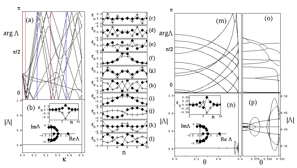
Figure 1: (Color online) Phases (a) and moduli (b) of Floquet eigenvalues as function of $\kappa$ for $E_{1}=0.05$, $\alpha=0.1$, and $\omega=0.35$. Floquet eigenvectors [panels (c)-(l)] at $E_{1}=0.05$, $\kappa=0.1$ (see text for details). Panels (m)-(p) show the phases and moduli of Floquet eigenvalues at $\kappa=0.1$ as function of $E_{1}$. Upper inset in panel (b) shows the eigenvector for unstable eigenvalue at $\kappa=0.5058245$ [${\mbox{R}e}~{}\varepsilon_{n}$ ($+$) and ${\mbox{I}m}~{}\varepsilon_{n}$ ($\blacklozenge$)]. Same for the inset in panel (n) at $E_{1}=0.58183325$. The lower insets shows the positions of eigenvalues.

Note that the eigenvalues are placed on the complex plane symmetrically with respect to the real axis, thus we limit ourselves with the eigenvalues lying in the upper half-plane ($\mbox{Re}\Lambda\geq 0$). The bias amplitude now is $E_{1}=0.05$, so that the excitations on the fluxon background can be treated as small. In the anticontinuum limit, all the eigenvalues sit in one point and with the growth of $\kappa$ they separate forming two distinct groups: the modes associated with the linear spectrum (Josephson plasmons) and the internal mode(s). The plasmon band extends linearly with $\kappa$ according to the dispersion law

$$\omega_{L}(q)=\sqrt{1+4\kappa~{}\sin^{2}\frac{q}{2}}~{}.$$ (8)

Due to finiteness of the array, the wavenumber $q\in[0,2\pi)$ attains only discrete set of values $q_{m}=2\pi m/N$, $m=\pm 1,\ldots,\pm N$. The localized eigenmode detaches itself from the linear band: as it is well known in the discrete Klein-Gordon theory Baesens et al. (1998), the internal mode is soft, so that it detaches from the linear band into the gap. In panels (c)-(l) of Fig. 1, the shapes of the eigenvectors ${\vec{\varepsilon}}$ (both real and imaginary parts) are shown for the parameter values $E_{1}=0.05$ and $\kappa=0.1$. These eigenvectors are ordered from top to bottom according to the decrease of $\arg\Lambda_{n}$. From the shape of the eigenvectors one can conclude that all of them, except one, are delocalized and therefore they are associated with the linear spectrum. The eigenmode in Fig. 1(f) has a clear localized structure. In our case, the fluxon state is locked to the external drive with the frequency $\omega=0.35$ which lies in the gap of the spectrum (8). Only the overtones $n\geq 3$ can lie in the linear spectrum: $1<n\omega<\sqrt{1+4\kappa^{2}}$, therefore the excited linear modes satisfy the condition $n\omega=\omega_{L}(q_{m})$, $m=1,2,\ldots,N$. The increase of $\kappa$ widens the linear spectrum and, as a result, the respective eigenvalues spread around the $R$-circle. The collisions of the eigenvalues at $\arg\Lambda=\pi$ with the highest ($m=N$) linear mode are marked by the vertical red lines at $\kappa=[(7\omega/2)^{2}-1]/4$ and $\kappa=[(9\omega/2)^{2}-1]/4$. They correspond to the parametric resonances of this mode with the external drive: $\omega_{L}(q_{N})=7\omega/2$ and $\omega_{L}(q_{N})=9\omega/2$. Collisions at $\arg\Lambda=0$ marked by the blue lines at $\kappa=[(3\omega)^{2}-1]/4$ and $\kappa=[(4\omega)^{2}-1]/4$ and correspond to the main resonances $\omega_{L}(q_{N})=4\omega$ and $\omega_{L}(q_{N})=4\omega$. The internal mode evolution with varying $\kappa$ can be clearly seen due to its nonlinear behavior as a function of $\kappa$, as compared to the linear evolution of plasmon modes. After interactions with the linear spectrum (marked by the avoided crossings), the internal mode hits the real axis at $\arg\Lambda=0$, thus signaling the resonance with some overtone of the driving frequency. After that the eigenvalue increases extremely fast [note the almost vertical growth of $|\Lambda_{n}|$ in Fig. 1(b)], leaves the $R$-circle and finally exits the unit circle. We conclude that the disappearance of the standing mode-locked fluxon takes place via the tangential (saddle-node) bifurcation. The excitation of the fluxon along the destabilizing direction in the phase space leads to chaotic fluxon diffusion with the net zero velocity.

While the previous investigation took place at rather small amplitudes for which the excitation on the fluxon background can be considered as small, now we focus on the evolution of the Floquet eigenvalues as a function of the driving amplitude for the fixed value of coupling $\kappa=0.1$. As one can see in Fig. 1(m-n), the eigenvalue that corresponds to the localized mode moves on the $R$-circle in the direction opposite to the motion of the linear band. After following the respective eigenvalue as a function of $E_{1}$, we see that it collides with its complex conjugated counterpart at $\arg\Lambda=\pi$ (see the resulting “bubble” in the $|\Lambda(E_{1})|$ dependence), continues its motion along the $R$-circle, then interacts with the eigenmodes of the linear spectrum and finally collides with its complex conjugate counterpart on the real axis but at $\arg\Lambda=0$. Next, the modulus of this eigenvalue grows fast and finally exceeds the unit circle. Again, the standing mode-locked fluxon state disappears via the tangential bifurcation. The unstable eigenvector is again spatially localized (see the inset in Fig. 1n). The perturbation of the kink in the unstable direction leads to the growth of a localized oscillation on the kink background that results in the kink-antikink pair birth and eventual destruction of the one-soliton state. Other scenarios are also possible. Similar investigation for the case $\kappa=0.2$ shows that the system can undergo additional bifurcations and a new standing mode locked fluxon can appear with a slightly different shape. However, the final disappearance of the standing kink goes similarly to the above scenario via the tangential bifurcation. In this case, the time evolution of the unstable fluxon turns into chaotic diffusive jumps of the kink backward and forward with the net zero velocity.

The main conclusion of this subsection is that standing mode-locked fluxon states disappear via a tangential bifurcation, when the driving amplitude $E_{1}$ or the coupling constant exceeds some critical value. The resulting dynamics can either lead to fluxon chaotic diffusion or to chaotic motion of the whole lattice and consequent fluxon destruction. Our analysis with $N=20$ and $N=30$ has shown that the size effects are insignificant: the critical values at which the tangential bifurcation takes place differ very slightly. The instability evolves via the excitation of a localized internal mode. This is in accordance with the previous results Salerno and Quintero (2002); Morales-Molina et al. (2003); Zolotaryuk and Salerno (2006) on the internal mode role in the kink mobility. More details on the kink response to the single harmonic ac drive (including the kink dynamics) can be found in Ref. Martínez et al. (1997). In particular, it has been shown that in the unlocking limit the kink dynamics shows the type-I intermittency.

V Asymmetric fluxon depinning

Now we focus on the main task of this paper, namely on the studies of the fluxon motion when the bias (2) is biharmonic ($E_{2}\neq 0$). Here and further on, we take $E_{1}=E_{2}$ unless stated otherwise. According to the previous studies Zolotaryuk and Salerno (2006); Cuevas et al. (2010), the fluxon motion becomes unidirectional due to the symmetry breaking and its average velocity depends solely on the system parameters. Also, from those papers we already know that critical parameter values should exist above which the applied external bias overcomes the forces of pinning and the fluxon starts to propagate. In particular, such critical values exist for the amplitudes of the external drive $E_{1,2}$ and the phase shift $\theta$.

Including the second harmonic in the bias (2), we add the third parameter (the phase shift $\theta$) into consideration and consequently we must think about the existence diagram in the three-dimensional parameter space $(\kappa,E_{1},\theta)$. However, since the average voltage drop satisfies $V(\theta)=V(\theta+2\pi)$, it is possible to construct the existence diagram on the plane $(\kappa,E_{1})$. This diagram for the existence of moving fluxon states is shown in Fig. 2. The numerical experiment has been performed as follows: the pinned state with the fluxon oscillating around its center of mass has been continued with small increase of $E_{1}$ or $\kappa$ until this state loses stability and starts to propagate. Transporting trajectories are mostly chaotic, but regular mode-locked trajectories may also exist. These trajectories will be analyzed in detail in the next subsections. As one can see, similarly to the case of the single harmonic drive, there exists a curve $E^{(c)}_{1}=E^{(c)}_{1}(\kappa)$ ( shown by markers) that separates the pinned and transporting parts of the diagram. In the area down and to the left from the curve $E^{(c)}(\kappa)$, there are only mode-locked standing fluxons and no mobile fluxons exist ($V\equiv 0$) for any $\theta\in[0,2\pi)$. The area to the right side of the curve corresponds to the situation where moving fluxons

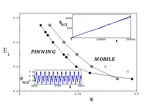
Figure 2: (Color online). Existence diagram of moving fluxons on the plane $(\kappa,E_{1})$ at $\alpha=0.1$ for $\omega=0.25$ ($\oplus$), $\omega=0.35$ ($\blacklozenge$) and $\omega=0.5$ ($\times$). Solid lines are used as a guide for an eye (see text for details). The upper and lower insets show the time evolution of the central junction for $\theta=2.5$, $\omega=0.35$, $\alpha=0.1$ and $\kappa=0.12$, $E_{1}=E_{2}=0.22$ (lower inset) and $\kappa=0.09$, $E_{1}=E_{2}=0.27$ (upper inset). Different colors correspond to different initial times: $t_{0}=0$ (black) and $t_{0}=\pi/\omega$ (blue).

($V\neq 0$) exist for some values of $\theta$. Obviously, in the continuum limit $\kappa\to\infty$, the critical depinning amplitude tends to zero, while in the anticontinuum limit $\kappa\to 0$, it is necessary to increase the driving amplitude in order to unlock the fluxon. At some point the critical drive is too strong and the fluxon is destructed due to the fluxon-antifluxon pair creation and the chaotic dynamics of the whole lattice. An example of such a pinned mode-locked trajectory is shown in the lower inset of Fig. 2. Note that the pinning to the lattice is independent on the initial conditions. For example, in this figure two trajectories with the initial times $t_{0}=0$ and $t_{0}=T/2$ are shown. Also, the scenario is the same for other values of initial time $t_{0}\in[0,T)$, the initial fluxon position, and different initial kicks. The examples of transporting chaotic trajectories with different initial times ($t_{0}=0$ and $t_{0}=T/2$) are illustrated by the upper inset of Fig. 2. Independently of the initial conditions at $t\to\infty$, the system settles on the chaotic attractor that corresponds to the directed fluxon motion with the same average velocity (in this case $V\simeq 0.0055$).

Note that the principal characteristics of the $E^{(c)}_{1}(\kappa)$ dependence remain qualitatively the same for different values of $\omega$. It has been shown in Ref. Zolotaryuk and Salerno (2006) that the ratchet fluxon motion is well pronounced in the frequency range $0\leq\omega\lesssim\omega_{L}(0)/2$. The Peierls-Nabarro frequency (which equals the frequency of the internal mode Braun et al. (1997)) at $\kappa=0.1$ (according to the relation $\omega_{PN}\simeq\sqrt{2\pi\alpha_{0}\kappa^{3/2}}\exp{(-\pi^{2}\sqrt{\kappa}/2)}$, $\;\;\alpha_{0}\simeq 30\pi\;$, see Ref. Ishimori and Munakata (1982)) equals $\omega_{PN}\simeq 0.91$. Thus, for small couplings the working frequency range lies below all characteristic system frequencies. Among the other system parameters the coupling constant and dissipation depend on the physical characteristics of the specific array and therefore they cannot be changed easily in the experiment. Consequently, we are left with the bias parameters $E_{1}$ and $\theta$ which can be tuned at will. Therefore it would be of interest to study the depinning process as a function of $\theta$ (with other parameters fixed) and the same for $E_{1}$. The following subsections will be devoted to this task.

V.1 Depinning as a function of the bias amplitude

For continuous ratchets it was shown previously Salerno and Zolotaryuk (2002) that the average kink velocity is proportional to $E_{1}^{2}E_{2}$, so that, provided the respective symmetries are broken, the directed motion can occur for arbitrary small values of the driving amplitudes. For the DSG equation, the dependence of the average kink velocity on the driver amplitudes is not a smooth monotonic function of $E_{1,2}$, but a complex function that either entirely or partially consists of plateaux of different lengths that correspond to mode-locked fluxon states. At $\kappa\gtrsim 1$ this dependence resembles closely a “devil’s staircase”, while this resemblance disappears when $\kappa$ is decreased leaving only isolated islands of regular motion Zolotaryuk and Salerno (2006).

In Fig. 3, the dependence of the Floquet eigenvalues on the driving amplitude is shown for different values of $\kappa$.

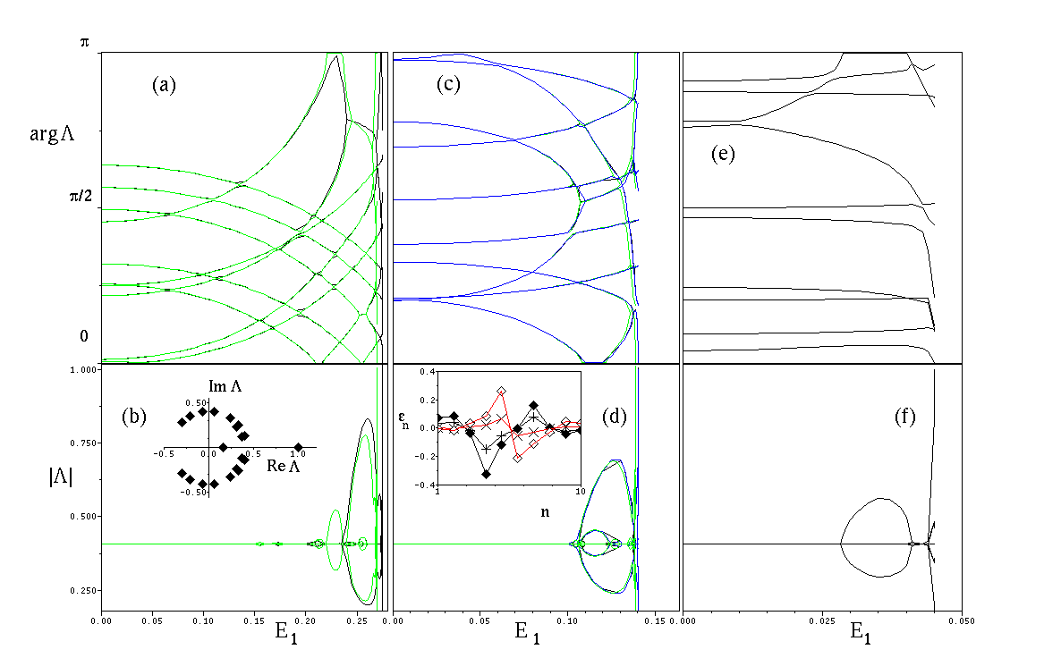
Figure 3: (Color online). Dependence of the phases (upper figures) and moduli (lower figures) of Floquet eigenvalues on bias amplitude $E_{1}$ at $\alpha=0.1$, $\omega=0.35$, and for different coupling constants and $\theta$: $\kappa=0.09$ (a-b), $\theta=1.5$ (black lines), $\theta=0$ (green lines); $\kappa=0.2$, (c-d), $\theta=1.5$ (black lines), $\theta=0$ (green lines); $\theta=-1.64159$ (blue lines); $\kappa=0.5$, $\theta=1.5$ (e-f). The inset in panel (b) shows the position of Floquet eigenvalues on complex plane at $E_{1}=0.04511641$. The inset in panel (d) shows the profile of unstable eigenvectors $\mbox{Re}\varepsilon_{n}$ ($+$) and $\mbox{Im}\varepsilon_{n}$ ($\blacklozenge$) at $E_{1}=0.1403205$, $\theta=1.5$ for eigenvalue $\Lambda=1.005497$ (black lines) and $E_{1}=0.14032053$, $\theta=-1.64159$ (scaled by $2$, red lines) for eigenvalue $\Lambda=1.000515$ [$\mbox{Re}\varepsilon_{n}$ ($\times$) and $\mbox{Im}\varepsilon_{n}$ ($\diamond$)]. Solid lines are used as guides for an eye.

Comparing Figs. 1(m-n) and 3(a-b), we observe the close similarity in the Floquet eigenvalue behavior in the single harmonic and biharmonic biased cases. It appears also that independently on the coupling strength, the loss of stability of the limit cycle appears through a collision of two eigenvalues at $\arg\Lambda=0$ and the departure of one of the eigenvalues out of the unit circle [see the inset in Fig. 3(b)] that signals a tangential bifurcation taking place at some critical value of the driving amplitude. This critical value decreases with the growth of $\kappa$. Note that the critical value of the bias amplitude is approximately two times smaller than in the single harmonic case because now the bias consists of two harmonics with the amplitude $E_{1}$. In panels (a-b), it should be noted that before the tangential bifurcation several period-doubling bifurcations take place that can easily be identified by the bubble-like deviations on the dependence $|\Lambda_{n}(E_{1})|$ from the value $|\Lambda_{n}|=R$. The amplitude of these deviations does not exceed the value $|\Lambda|=1$ and they decrease with $\kappa$, so that the limit cycle remains stable. At higher $\kappa=0.2$, the largest bubble corresponds to a pair of eigenvalues colliding away from the real axis (that corresponds to the Hopf bifurcation). For even higher $\kappa=0.5$, again a bubble associated with the period-doubling bifurcation can be seen. Although for the given range of parameters these bifurcations do not cause instability of the limit cycle, the increase of $\omega$ or decrease of $\alpha$ may change the nature of the depinning transition. The computations have been performed for different values of $\theta$ and the dependencies $\Lambda_{n}(E_{1})$ appear to be rather similar since the curves of different colors almost coincide. The only difference lies in the different critical values of $E_{1}$, when the tangential bifurcation takes place, however these differences are rather small.

The unstable eigenvector, shown in the inset of panel (d) has a pronounced localized asymmetric shape. The eigenvectors that correspond to the opposite (with respect to the shift $\theta\to\theta\pm\pi$) values $\theta=1.5$ and $\theta=1.5-\pi\simeq-1.64159$ are related to each other approximately by the inversion ${\bf\varepsilon}\to-C{\bf\varepsilon}$, where $C$ is an arbitrary constant that appears because Eqs. (6) are linear. This means that the unstable perturbation drives the fluxon in the opposite directions for $\theta$ and $\theta+\pi$, respectively.

The behavior of the eigenvalues in the parameter space $(\kappa,E_{1},\theta)$ has very complicated structure. In particular, it is possible that for some values of $\theta$, the standing fluxon states can exist after the tangential bifurcation shown in Fig. 3. For the sake of brevity, we are going to refer to it as to the first tangential bifurcation. Indeed, such an example is given by Fig. 4. After the firts tangential bifurcation, the standing solution (limit cycle) becomes unstable at $E_{1}\simeq 0.2357$ and soon disappears but reappears back after another tangential bifurcation. In the short interval between these bifurcations, a chaotic moving fluxon appears. The further increase of the driving amplitude leads to the Hopf bifurcation (collision of two eigenvalues on the complex plane) and to the eventual departure of two eigenvalues out of the unit circle. This instability leads to formation of a large localized excitation on the fluxon and the eventual creation of fluxon-antifluxon pairs. Thus, it is possible to pass from the pinned area to the non-existing area (where no fluxons exist due to chaos) omitting the transporting area (where the moving fluxons exist).

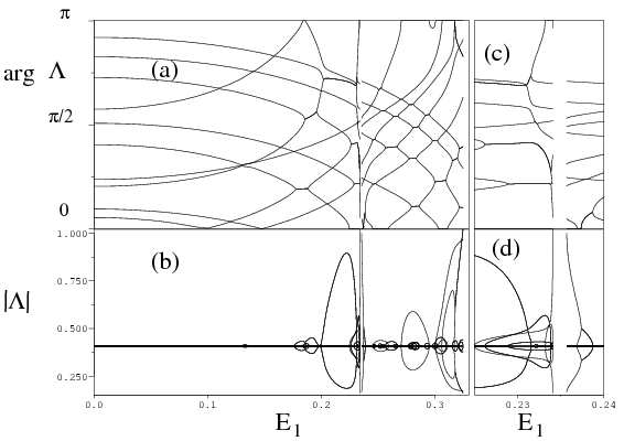
Figure 4: Phases (a) and moduli (b) of Floquet eigenvalues as a function for $\omega=0.35$, $\alpha=0.1$, $\kappa=0.12$, $\theta=1.5$. Panels (c) and (d) give details in interval $E_{1}\in$ $(0.22,0.24)$.

This bifurcation analysis explains the non-monotonous behavior of the average velocity dependence on the bias amplitude for small $\kappa$ (see Fig. 8 of Ref. Zolotaryuk and Salerno (2006)), when the intervals of zero and non-zero fluxons velocities interchange with the growth of $E_{1}$.

V.2 Depinning as a function of the phase shift

The directed fluxon transport in the continuous sine-Gordon model shows Salerno and Zolotaryuk (2002) that the dependence of the average fluxon velocity (and, consequently, the voltage drop) behaves as $\sin[\theta-\theta_{0}(\omega,\alpha)]$. As it has been shown in Ref. Zolotaryuk and Salerno (2006), in the weakly discrete case, the two values of $\theta$ where $V(\theta)=0$ become intervals, and the size of these intervals increases when $\kappa$ decreases. Moreover, the dependence $V(\theta)$ changes from the continuous behavior into the complex piecewise function which may include resonant plateaux $V=\omega k/(lN)$ and loses its resemblance with the sine function as long as $\kappa\to 0$. For $\kappa\gtrsim 1$ there exist at least two intervals on the $\theta$ axis which we denote as $(\theta^{-}_{1},\theta^{-}_{2})$ and $(\theta^{+}_{1},\theta^{+}_{2})$ where $V\neq 0$. In particular, $V(\theta)<0$ if $\theta\in(\theta^{-}_{1},\theta^{-}_{2})$ and $V(\theta)>0$ if $\theta\in(\theta^{+}_{1},\theta^{+}_{2})$. It appears, however, that for small $\kappa$ the dependence $V(\theta)$ may take a more complicated shape (for example, see Fig. 8 of Ref. Zolotaryuk and Salerno (2006)). This also can clearly be seen in the main graph of Fig. 5, where the dependencies for $V(\theta)$ for several values of $\kappa$ and for the fixed value of $E_{1}=0.27$ are given. This figure in some sense is complementary to Fig. 2 because it explains in detail what is happening around the curve $E^{(c)}_{1}(\kappa)$ when $\theta$ changes. While at $\kappa=0.09$ only two transporting intervals where $V\neq 0$ are observed with $\theta^{-}_{1}\simeq-0.69$, $\theta^{-}_{2}\simeq 0.23$ and $\theta^{+}_{1}\simeq 2.47$, $\theta^{+}_{2}\simeq-2.92$. For other values, namely, for $\kappa=0.12$ there can exist two additional transporting intervals. The transporting intervals (shown by vertical bars on the upper inset of Fig. 5) decrease as $\kappa\to 0$ at $E_{1}=\mbox{const}$. The same behavior occurs if $\kappa$ is fixed and $E_{1}$ decreased.

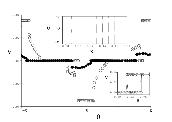
Figure 5: Average voltage drop as a function of phase shift $\theta$ for $\omega=0.35$, $\alpha=0.1$, $E_{1}=E_{2}=0.27$, $\kappa=0.09$ ($\blacklozenge$) and $\kappa=0.12$ ($\circ$). The upper inset shows the existence diagram of transporting trajectories (vertical bars) on plane $(\kappa,\theta)$. The lower inset shows the details of hysteresis (see text).

It is worth to notice the existence of regular transporting limit cycles that correspond to the constant voltage plateaux $V=\pm 0.035$ for $\kappa=0.12$. Their existence has been obtained by the direct Runge-Kutta integration of the equations of motion and also has been confirmed by the Newton method with $k=\pm 1$, $l=1$. The careful investigation of the transition between the pinned state and these plateaux shows the existence of narrow hystereses windows as shown in the lower inset of Fig. 5. In order to understand the nature of the additional pinning intervals, the Floquet analysis of the standing limit cycles has been performed as a function of $\theta$.

In Fig. 6 the behavior of the Floquet eigenvalues as a function of the desymmetrizing parameter $\theta$ for different values of $E_{1}$ below and above the depinning threshold is shown. The left panels (a-b) correspond to the situation when $\kappa=0.09$ and $E_{1}$ is increased from below the critical depinning dependence $E^{(c)}(\kappa)$. One can see that initially the curves $\arg\Lambda_{n}(\theta)$ do not cross each other. For $E_{1}=0.26$ all the eigenvalues lie on the $R$-circle except for the two pairs with $\arg\Lambda_{n}$ oscillating around $\pm 3\pi/2$ and having $|\Lambda_{n}|\neq R$, as it can clearly be seen from Fig. 6(a-b). These eigenvalues correspond to the spatially localized eigenvectors as shown in Fig. 6(c). Moreover, the non-localized eigenvalues are virtually independent on $\theta$. The shape of the localized eigenvectors does not differ significantly for $\theta=\pm\pi$ and $\theta=0$ as well. A slight increase of the driving amplitude to the value $E_{1}=0.265$ leads to further increase of the oscillation of localized eigenvalues.

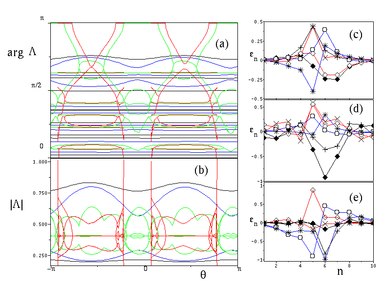
Figure 6: (Color online). Phases (a) and moduli (b) of eigenvalues of Floquet matrix as a function of phase delay $\theta$ for $\omega=0.35$, $\kappa=0.09$ and $E_{1}=E_{2}=0.26$ (black), $E_{1}=E_{2}=0.265$ (blue), $E_{1}=E_{2}=0.269$ (green) and $E_{1}=0.27$ (red). Panels (c)-(e) show the real and imaginary parts of destabilizing eigenvectors the eigenvalues that lie out of the $R$-circle (see text for details): (c) $E_{1}=0.26$ with $\theta=-\pi$ [red, $\mbox{Re}~{}\varepsilon$ ($\times$), $\mbox{Im}~{}\varepsilon$ ($\diamond$)], $\theta=-\pi/2$ [blue, $\mbox{Re}~{}\varepsilon$ ($*$), $\mbox{Im}~{}\varepsilon$ ($\circ$)] and $\theta=0$ [black,$\mbox{Re}~{}\varepsilon$ ($+$), $\mbox{Im}~{}\varepsilon$ ($\blacklozenge$)]; (d) $E_{1}=0.269$ (the same); (e) $E_{1}=0.27$ with $\theta=-2.914$ [red, $\mbox{Re}~{}\epsilon$ ($\times$), $\mbox{Im}~{}\varepsilon$ ($\diamond$)], $\theta=-\pi/2$ [blue, $\mbox{Re}~{}\varepsilon$ ($*$), $\mbox{Im}~{}\varepsilon$ ($\circ$)] and $\theta=-0.69206$ [black, $\mbox{Re}~{}\varepsilon$ ($+$), $\mbox{Im}~{}\varepsilon$ ($\blacklozenge$)].

Upon the further increase of $E_{1}$, the eigenvalue collisions at $\Lambda=-1$ and out of the real axis take place (see, for example, the green line in Fig. 6(a) that corresponds to $E_{1}=0.269$). The monitoring of the eigenvectors that correspond to the eigenvalues with $|\Lambda_{n}|\neq R$ (see panel (d) of Fig. 6) shows that the eigenvector shape changes significantly, although they remain spatially localized. Now the phases of all the eigenvalues demonstrate significant dependence on $\theta$. The crossings of the $\arg\Lambda_{n}(\theta)$ curves demonstrate that the localized eigenmode “interacts” with the modes of the linear spectrum. First of all we note the collision of the eigenvalues at $\arg\Lambda=\pi$ that corresponds to the period-doubling bifurcation. These bifurcations are clearly seen if one compares the lines for $E_{1}=0.265$ and $E_{1}=0.269$ in Fig. 6(a-b), however, they do not cause any instabilities. After reaching some critical value of $E_{1}$, the localized eigenvalues which previously have resided in the complex plane collide with each other on the real axis at ${\mbox{Re}}\Lambda>0$. The further increase of $E_{1}$ leads to the fast exit of one of them out of the unit circle and to the subsequent tangential bifurcation. Beyond this bifurcation point, the non-transporting limit cycle disappears. For $E_{1}=0.27$ there exist four tangential bifurcations, two direct and two inverse, that happen not far from the values $\theta=0$ and $\theta=\pm\pi$. The respective unstable eigenvectors are spatially localized, as shown in Fig. 6(e). The respective repeller also has been computed (not shown in the figure for the sake of clearness), and its eigenvalues join the attractor eigenvalues at the bifurcation point. The transporting intervals $(\theta_{1}^{-},\theta_{2}^{-})$ and $(\theta_{1}^{+},\theta_{2}^{+})$ in Fig. 5 for $\kappa=0.09$ obviously correspond to the windows in Fig. 6(a-b) where the standing fluxon does not exist. Similarly to the dependencies shown in Fig. 3, the bifurcation points are preceded by the sharp singular-like growth of the modulus of the unstable eigenvalue.

A different scenario is presented in Fig. 7. As it has been discussed in the previous subsection, the existence subspaces of the transporting and non-transporting trajectories in the parameter space $(\kappa,E_{1},\theta)$ can take a peculiar and complicated shape. This is also true for the discrete soliton ratchets with the spatial symmetry breaking studied in Ref. Cuevas et al. (2010) (see Fig. 12 therein). If one stays above the critical dependence $E_{1}^{(c)}(\kappa)$, it is possible to observe the existence of a non-transporting limit cycle after the first tangential bifurcation as shown in Fig. 4. It is logical to investigate such a case for different $\theta$’s when $E_{1}>E_{1}^{(c)}(\kappa)$. This exactly has been done in Fig. 7 where the eigenvalue behavior has been plotted as a function of $\theta$ for $E_{1}=0.25$ and $E_{1}=0.27$. On these figures again four tangential bifurcations are seen (two direct and two inverse), clearly pointing out the windows where the directed fluxon motion takes place. These bifurcations are characterized by sharp singular growth of the respective $|\Lambda_{n}(\theta)|$ dependencies.

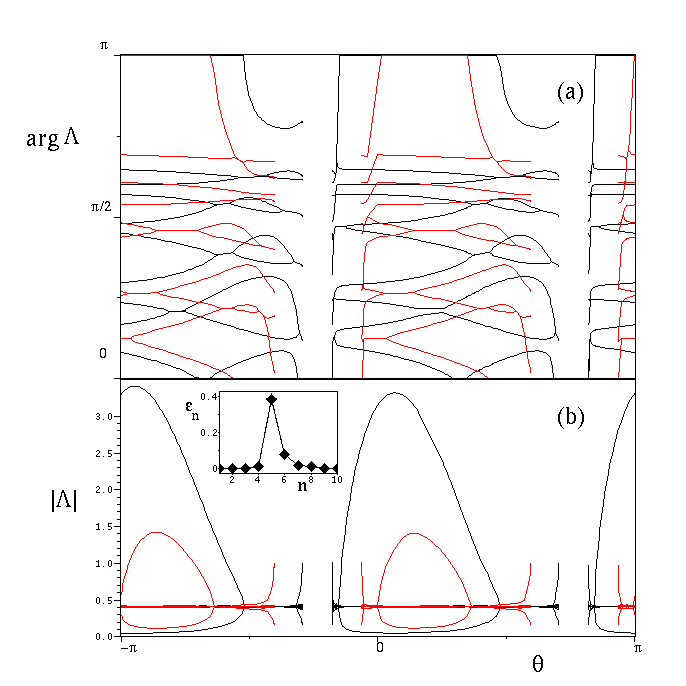
Figure 7: (Color online). Phases (a) and moduli (b) of eigenvalues of Floquet matrix as a function of phase delay $\theta$ for $\kappa=0.12$, $E_{1}=E_{2}=0.25$ (red) and $E_{1}=E_{2}=0.27$. The rest of parameters is as in Fig. 6. The inset shows the unstable eigenvector ${\mbox{Re}}~{}\varepsilon$ ($+$) and ${\mbox{Im}}~{}\varepsilon$ ($\blacklozenge$) at $\theta=-3.03$ just after the period-doubling bifurcation (see text for details).

Apart from these bifurcations which are typical for the case considered before (including Fig. 6), the two large “bubbles” on the dependence $|\Lambda_{n}(\theta)|$ can be noticed. They correspond to the eigenvalue collisions on the real axis at $\mbox{Re}~{}\Lambda_{n}<0$ and to the subsequent departure of one of them out of the unit circle. Thus, we observe period-doubling bifurcations that make the mode-locked state ustable. Along the interval $\pi\leq\theta<\pi$ the four period-doubling bifurcations take place: two direct and two inverse. The destabilizing eigenvector is spatially localized as in the case of tangential bifurcations (see the inset of Fig. 7). Note that the “bubbles” of the instable eigenvalues increase when $E_{1}$ increases. The stable period-2 (with $l=2$) limit cycles that appear after the bifurcation, have been computed with the Newton method until the next period-doubling bifurcation takes place. The emerging period-4 cycle has been computed as well. In the next section, it will be shown that in fact the cascade of period-doubling bifurcations takes place leading to chaotic dynamics.

Now we can explain why the dependence $V(\theta)$ computed in Fig. 5 for $\kappa=0.12$ has not two but four transporting intervals. The old transporting intervals $(\theta_{1}^{+},\theta_{2}^{+})$ and $(\theta_{1}^{-},\theta_{2}^{-})$ now have non-transporting windows embedded within them. The borders of these intervals are associated with the depinning of fluxons and they, of course, do not exactly coincide with the points of period-doubling bifurcations of Fig. 7. The actual depinning takes place after the sequence of the period-doubling bifurcations and transition to chaotic dynamics.

V.3 Dynamical properties of depinned trajectories

Thus, we have seen that the loss of stability of a pinned mode-locked fluxon takes place either due to a tangential bifurcation or after a sequence of period-doubling bifurcations. In this subsection, we focus on the fluxon dynamics at the depinning threshold.

Consider first the case of mode-locked state stability loss via the tangential bifurcation as the phase shift $\theta$ varies. In this case, we consider the already unstable mode-locked state with one of the eigenvalues slightly out of the unit circle. After perturbing this state in the direction of the unstable eigenvector, the directed fluxon propagation begins. It has clear chaotic nature as shown in Fig. 8(a).

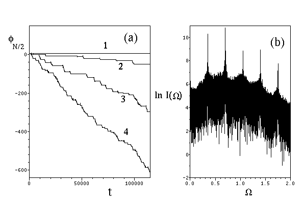
Figure 8: Panel (a). Time evolution of central junction phase $\phi_{N/2}$ at $\kappa=0.12$, $E_{1}=E_{2}=0.27$, $\omega=0.35$, $\alpha=0.1$ for $\theta=-0.92462$ (1), $\theta=-0.9246$ (2), $\theta=-0.9245$ (3), and $\theta=-0.924$ (4). Panel (b) shows power spectrum for $\theta=-0.924$.

The fluxon dynamics takes place according to the intermittency type-I scenario: the junction phase (in this case the central one with $n=N/2$) oscillates regularly around the equilibrium position as shown by the plateaux of constant phase $\phi_{N/2}$ and then suddenly jumps in a certain direction of propagation (sometimes after several chaotic back and forward jumps). The average length of the regular (laminar) plateaux is inversely proportional to the voltage drop. This length decreases as $\theta$ moves away from the bifurcation point. Note the extremely sharp dependence of the modulus of the unstable eigenvalue $|\Lambda_{unst}|$ as a function of $E_{1}$ and $\theta$ in Figs. 3 and 6, respectively. Since the length of the laminar regime is proportional to $1/(|\Lambda_{unst}|-1)$, it is necessary to change the respective parameter in the neighborhood of the depinning transition with very small increments. Due to limited computing power this procedure was not done and, as a result, the dependencies in Fig. 5 seem to start “out of nowhere”.

The power spectrum of the junction’s phase velocity defined as

$$I(\Omega)=\left|\int_{-\infty}^{+\infty}{\dot{\phi}}_{N/2}(t)e^{-i\Omega t}dt\right|^{2},$$ (9)

has been computed in Fig. 8(a). The sharp peaks are located at the multiples of the driving frequency: $\Omega=n\omega$, $n=1,2,\ldots$. These peaks clearly illustrate the remnants of the mode-locked dynamics before the tangential bifurcation. The type-I intermittency in the depinning transition for the single-harmonically driven kinks has been observed in Ref. Martínez et al. (1997).

Now we focus ourselves on the depinning scenario due to the period-doubling bifurcations. Consider the case depicted in Fig. 7 when the standing fluxon loses its stability via the period-doubling bifurcation, for example, at $\kappa=0.12$, $\theta\simeq-1.85$. The further decrease of $\theta$ leads to the sequence of period-doubling bifurcations where the initially stable $2T$, $4T$, $\ldots$ cycles lose their stability. A typical period-doubling route to chaos takes place and the standing fluxon becomes quasiperiodic and later chaotic. With decrease of $\theta$, the amplitude of chaotic oscillations grows and the fluxon starts to propagate. In Fig. 9(a) the typical trajectories after the depinning point are shown. Curve 1 corresponds to non-transporting trajectories both regular and chaotic. Since they overlap, the inset with the Poincare sections, computed on the plane $\{\phi_{N/2},{\dot{\phi}}_{N/2}\}$ at every time interval $t_{n}=nT$, $n=1,2,\ldots$ is presented. Curves $2-4$ correspond to transporting trajectories. The dynamical fluxon trajectories have the structure similar to the case described in the previous paragraph. They consist of long intervals, where the fluxon stays pinned, which are interrupted by short chaotic bursts. During these bursts (which occur at random) the fluxon jumps normally in the direction specified by the asymmetry of the bias function $E(t)$.

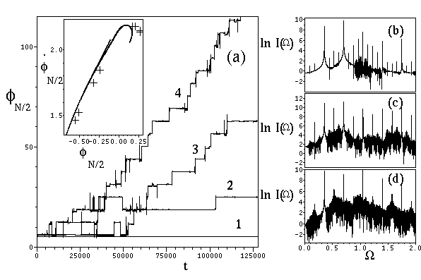
Figure 9: Panel (a). Time evolution of the central junction phase $\phi_{N/2}$ at $\kappa=0.12$, $E_{1}=E_{2}=0.27$, $\omega=0.35$ for $\theta=-2.08$ (1), $\theta=-2.11$ (2), $\theta=-2.115$ (3) and $\theta=-2.12$ (4). The inset shows the Poincare section for $\theta=-2.045$ ($+$) and $\theta=-2.08$ (dots). Panels (b)-(d) show Fourier power spectra for $\theta=-2.05$ (b), $\theta=-2.055$ (c) and $\theta=-2.08$ (d).

Sometimes a series of forward and backward jumps takes place. Again, the length of the pinned intervals decreases as $\theta$ moves away from the critical depinning value. These dynamical pictures bear a significant difference, although they look similar. In the first case, the standing fluxons are always regular and the transporting trajectory is chaotic with long regular intervals where dynamics is very close to the periodic one with the period $T$. In the depinning scenario, driven by the period-doubling bifurcations, the chaotization happens before depinning and the stationary intervals of the depinned trajectories cannot be called laminar because their structure is in fact chaotic.

The power spectra in Fig. 9(b-d) clearly indicate the period-doubling route to chaos. Indeed, apart from the peaks at $n\omega$, $n=1,2,\ldots$, one can clearly see the peaks at $n\omega\pm m\omega/2$ and $n\omega\pm m\omega/4$, $m,n=1,2,\dots$, in Fig. 9(b). As $\theta$ decreases into the chaotic region, the peaks that correspond to the $\omega/4$ contribution get smeared out and only the $\omega/2$ peaks survive [see panel (c)]. After the further decrease of $\theta$ the subharmonic peaks become even less pronounced.

VI Discussion and conclusions

In this paper, we have studied the fluxon dynamics in a highly discrete annular Josephson junction array driven by the asymmetric periodic bias current with the zero mean value. It is already well-known that this bias (consisting of a cosine harmonic and its second overtone) leads to a directed fluxon motion which is manifested by the non-zero voltage drop. It is interesting to note that for the strongly discrete JJA the ratchet transport is mainly chaotic, while the non-transporting states are regular. Thus, the chaotic dynamics can be identified experimentally directly from the IV curves.

We mainly focus on the depinning process of the fluxon in the limit of the weak coupling between the neighboring junctions ($\kappa\ll 1$). It appears that the fluxon motion is possible in this case provided the amplitude of the ac bias is sufficiently large. The existence diagram on the parameter plane $(\kappa,E_{1})$ has been computed. On this plane, the curve $E^{(c)}(\kappa)$ separates the area where only mode-locked standing fluxons exist for any phase shift $\theta$ from the area where moving fluxons can exist for some values of $\theta$. In fact, this diagram can be treated as the projection of a more complicated three-dimensional parameter space $(\kappa,E_{1},\theta)$ on the plane $(\kappa,E_{1})$.

We have investigated the depinning of the initially standing mode-locked fluxon state not far from the critical line $E_{1}^{(c)}(\kappa)$ by analyzing its Floquet spectrum. The depinning occurs through chaotization of the mode-locked state. The mechanisms of chaotization are diverse and depend on the initial position of the non-transporting limit cycle in the parameter space $(\kappa,E_{1},\theta)$. The most common depinning scenario occurs through the type-I intermittency which evolves after the tangential bifurcation destroys a standing fluxon limit cycle. This scenario is ubiquitous when approaching the $E_{1}^{(c)}(\kappa)$ curve from below by increasing the bias amplitude $E_{1}$. Another scenario develops through a sequence of period-doubling bifurcations. It happens slightly above the $E_{1}^{(c)}(\kappa)$ curve when $\theta$ is varied.

Finally, we would like to point out some further research directions. The main difficulty in studying the kink dynamics in strongly discrete systems is the lack of an adequate analytical approximation. As a result, we are forced to work with numerical methods. The existing approximate theories are based on the perturbations of the continuum models where kinks are treated as point particles (maybe with the internal mode taken into account) in the PN potential. This approach works relatively well if $\kappa\gtrsim 1$ but breaks if $\kappa\ll 1$. An important tool that could help to obtain the $E_{1}^{(c)}(\kappa)$ curve analytically is the Melnikov criterion. However, the effectively use of it requires the explicit expressions for the stable and unstable manifolds in order to build the Melnikov function. For example, successful implementation of the Melnikov method used in Ref. Martínez and Chacón (2004); Chacón and Martínez (2007) utilizes the collective coordinate approximation which is not applicable in our case. Performing the same for the case of small $\kappa$ in our opinion is an important challenge.

In summary, we remark that the biharmonically driven ratchet effect in JJAs is robust phenomenon that takes place even in the limit of very strong coupling between the neighboring junctions.

VII Acknowledgements

Financial support from DFFD (grant F35/544-2011) is acknowledged.

References

- Watanabe et al. (1996) S. Watanabe, H. S. J. van der Zant, S. H. Strogatz, and T. P. Orlando, Physica D 97, 429 (1996).
- Ustinov (1998) A. V. Ustinov, Physica D 123, 315 (1998).
- Floria and Mazo (1996) L. M. Floria and J. J. Mazo, Adv. Phys. 45, 505 (1996).
- Braun and Kivshar (1998) O. M. Braun and Y. S. Kivshar, Phys. Rep. 306, 2 (1998).
- (5) S. Shapiro, Phys. Rev. Lett. 11, 80 (1963); S. Shapiro, A. R. Janus, and S. Holly, Rev. Mod. Phys. 36, 223 (1964).
- (6) R. L. Kautz, J. Appl. Phys. 52, 3528 (1981).
- (7) R. L. Kautz, J. Appl. Phys. 52, 6241 (1981); E. Ben-Jacob, Y. Braiman, R. Shainsky and Y. Imry, Appl. Phys. Lett. 38, 822 (1981); R. L. Kautz and R. Monaco, J. Appl. Phys. 57, 875 (1985);
- (8) R. L. Kautz, Rep. Prog. Phys. 59 (1996) 935.
- (9) M. T. Levinsen, R. Y. Chiao, M. J. Feldman and B. A. Tucker, Appl. Phys. Lett. 31, 776 (1977); R. L. Kautz, Appl. Phys. Lett. 36, 386 (1980).
- Braun et al. (2000) O. Braun, B. Hu, and A. Zeltser, Phys. Rev. E 62, 4235 (2000).
- (11) A. V. Ustinov, M. Cirillo and B. A. Malomed, Phys. Rev. B 47, 8357 (1993).
- (12) G. Filatrella and B. A. Malomed, J. Phys.: Condens. Matter 11, 7103 (1999).
- Glatz et al. (2003) A. Glatz, T. Nattermann, and V. Pokrovsky, Phys. Rev. Lett. 90, 047201 (2003).
- Nattermann et al. (2001) T. Nattermann, V. Pokrovsky, and V. M. Vinokur, Phys. Rev. Lett. 87, 197005 (2001).
- Jülicher et al. (1997) F. Jülicher, A. Ajdari, and J. Prost, Rev. Mod. Phys. 69, 1269 (1997).
- Reimann (2002) P. Reimann, Phys. Rep. 361, 57 (2002).
- Hänggi and Marchesoni (2009) P. Hänggi and F. Marchesoni, Rev. Mod. Phys. 81, 387 (2009).
- Flach et al. (2000) S. Flach, O. Yevtushenko, and Y. Zolotaryuk, Phys. Rev. Lett. 84, 2358 (2000).
- Denisov et al. (2002) S. Denisov, S. Flach, A. A. Ovchinnikov, O. Yevtushenko, and Y. Zolotaryuk, Phys. Rev. E 66, 041104 (2002).
- Barbi and Salerno (2000) M. Barbi and M. Salerno, Phys. Rev. E 62, 1988 (2000).
- Barbi and Salerno (2001) M. Barbi and M. Salerno, Phys. Rev. E 63, 066212 (2001).
- (22) W. Wonneberger, Z. Phys. B 53, 167 (1983).
- (23) R. Monaco, J. Appl. Phys. 68, 679 (1990).
- (24) M. Salerno, Phys. Rev. B 44, 2720 (1991).
- (25) G. Filatrella and G. Rotoli, Phys. Rev. B 50, 120802 (1994).
- (26) G. Carapella, Phys. Rev. B 63, 054515 (2001); G. Carapella and G. Costabile, Phys. Rev. Lett. 87, 077002 (2001).
- (27) M. Beck et al, Phys. Rev. Lett. 95, 090603 (2005).
- (28) D. E. Shalom and H. Pastoriza, Phys. Rev. Lett. 94, 177001 (2005).
- (29) J. F. Wambaugh et al., Phys. Rev. Lett. 83, 5106 (1999).
- (30) A. V. Ustinov et al., Phys. Rev. Lett. 93, 087001 (2004).
- Trías et al. (2000) E. Trías, J. J. Mazo, F. Falo, and T. P. Orlando, Phys. Rev. E 61, 2257 (2000).
- Falo et al. (1999) F. Falo, P. J. Martínez, J. J. Mazo, and S. Cilla, Europhys. Lett. 45, 700 (1999).
- Cuevas et al. (2010) J. Cuevas, B. Sánchez-Rey, and M. Salerno, Phys. Rev. E 82, 016604 (2010).
- Savin et al. (1997) A. V. Savin, G. P. Tsironis, and A. V. Zolotaryuk, Phys. Rev. E 56, 2457 (1997).
- Marconi (2007) V. I. Marconi, Phys. Rev. Lett. 98, 047006 (2007).
- Zolotaryuk and Salerno (2006) Y. Zolotaryuk and M. Salerno, Phys. Rev. E 73, 066621 (2006).
- Martínez and Chacón (2008) P. J. Martínez and R. Chacón, Phys. Rev. Lett. 100, 144101 (2008).
- Poletti et al. (2009) D. Poletti, E. A. Ostrovskaya, T. J. Alexander, B. Li, and Y. S. Kivshar, Physica D 238, 1338 (2009).
- Binder et al. (2000) P. Binder, D. Abraimov, A. V. Ustinov, S. Flach, and Y. Zolotaryuk, Phys. Rev. Lett. 84, 745 (2000).
- Arnol’d (1989) V. I. Arnol’d, Mathematical Methods of Classical Mechanics (Springer, Berlin, 1989).
- Miroshnichenko et al. (2001) A. E. Miroshnichenko, S. Flach, M. V. Fistul, Y. Zolotaryuk, and J. B. Page, Phys. Rev. E 64, 066601 (2001).
- Marín et al. (2001) J. L. Marín, F. Falo, P. Martínez, and L. M. Floría, Phys. Rev. E 63, 066603 (2001).
- Sepulchre and MacKay (1997) J. A. Sepulchre and R. S. MacKay, Nonlinearity 10, 679 (1997).
- Flach and Willis (1998) S. Flach and C. R. Willis, Phys. Rep. 295, 182 (1998).
- Peyrard and Kruskal (1984) M. Peyrard and M. D. Kruskal, Physica D 14, 88 (1984).
- Martínez et al. (1997) P. J. Martínez, F. Falo, J. Mazo, L. M. Floría, and A. Sánchez, Phys. Rev. B 56, 87 (1997).
- Baesens et al. (1998) C. Baesens, S. Kim, and R. S. Mackay, Physica D 113, 242 (1998).
- Salerno and Quintero (2002) M. Salerno and N. R. Quintero, Phys. Rev. E 65, 025602(R) (2002).
- Morales-Molina et al. (2003) L. Morales-Molina, N. R. Quintero, F. G. Mertens, and A. Sánchez, Phys. Rev. Lett. 91, 234102 (2003).
- Braun et al. (1997) O. Braun, Y. Kivshar, and M. Peyrard, Phys. Rev. E 56, 6050 (1997).
- Ishimori and Munakata (1982) Y. Ishimori and T. Munakata, J. Phys. Soc. Japan 51, 3367 (1982).
- Salerno and Zolotaryuk (2002) M. Salerno and Y. Zolotaryuk, Phys. Rev. E 65, 056603(10) (2002).
- Martínez and Chacón (2004) P. J. Martínez and R. Chacón, Phys. Rev. Lett. 93, 237006 (2004).
- Chacón and Martínez (2007) R. Chacón and P. J. Martínez, Phys. Rev. Lett. 98, 224102 (2007).