Period doubling and reducibility in the quasi-periodically forced logistic map

Abstract

We study the dynamics of the Forced Logistic Map in the cylinder. We compute a bifurcation diagram in terms of the dynamics of the attracting set. Different properties of the attracting set are considered, as the Lyapunov exponent and, in the case of having a periodic invariant curve, its period and its reducibility. This reveals that the parameter values for which the invariant curve doubles its period are contained in regions of the parameter space where the invariant curve is reducible. Then we present two additional studies to explain this fact. In first place we consider the images and the preimages of the critical set (the set where the derivative of the map w.r.t the non-periodic coordinate is equal to zero). Studying these sets we construct constrains in the parameter space for the reducibility of the invariant curve. In second place we consider the reducibility loss of the invariant curve as codimension one bifurcation and we study its interaction with the period doubling bifurcation. This reveals that, if the reducibility loss and the period doubling bifurcation curves meet, they do it in a tangent way.

1 Introduction

We focus on the study of the quasi-periodically (q.p. for short) Forced Logistic Map (FLM for short). The FLM is a two parametric map in the cylinder where the dynamics in the periodic component is a rigid rotation and the dynamics in the other component is the logistic map plus a quasi-periodic forcing term. This map appears in the literature in different contexts, usually related with the destruction of invariant curves. For example, in [13] it was introduced as an example where SNAs (Strange Non-chaotic Attractors) were created through a collision between stable and unstable invariant curves. Since then, different routes for the destruction of invariant curves have been explored for this map, for instance see [25] and references therein. Some other recent studies are [1, 2, 4, 10, 15, 20].

On the other hand, the FLM is also related to the truncation of period doubling cascades. It is well known that the one dimensional logistic map exhibits an infinite cascade of period doubling bifurcations which leads to chaotic behavior. Moreover this infinite cascade extends to a wider class of unimodal maps. But when some q.p. forcing is added, the number of period doubling bifurcations of the invariant curves is finite. This phenomenon of finite period doubling cascade has been observed in different applied and theoretical contexts. In the applied context it has been observed in a truncation of the Navier-Stokes flow [11, 28] or in a periodically driven low order atmosphere model [6]. In the theoretical context, it has also been reported in different maps which were somehow built to have period doubling cascades [3, 21], and more recently in the analysis of the Hopf-saddle-node bifurcation [7]. Actually, in [21] the FLM itself is given as a model for the truncation of the period doubling bifurcation cascade.

The study presented here is more concerned with the mechanisms which cause the truncation of the period doubling bifurcation cascades than with the possible existence of SNAs for this family of maps. Concretely, we show (numerically) that the reducibility has the role of confining the period doubling bifurcation in closed regions of the parameter space. In the remainder of this article we focus on the shape of this reducibility regions. In [17, 18, 19] we will use the reducibility loss bifurcation to study the self renormalizable properties of the bifurcation diagram and how the Feigenbaum-Collet-Tresser renormalization theory can be extended to understand it. See also [26] for a united exposition of the present paper with the other three cited before.

This paper is structured as follows. In section 2 we review some concepts and results concerning the continuation of invariant curves for a quasi-periodic forced maps. We also look at the concrete case when the map is uncoupled.

In section 3 we focus on the dynamics of the FLM. First we review some computations which can be found in the literature. Then, we do a study of the parameter space in terms of the dynamics of the attracting set of the map. For this study different properties of the attracting set are considered, as the value of the Lyapunov exponent and, in the case of having a periodic invariant curve, the period. Differently to other works, in our study the reducibility of the invariant curves has been also taken into account. This reveals interesting information, for example we observe that the parameter values for which the invariant curve doubles its period is contained in regions of the parameter space where the invariant curve is reducible. The subsequent sections are developed with the aim of understanding the results presented in this section.

In section 4 we consider the images and the preimages of the critical set (this set is the set where the derivative of the map w.r.t the non-periodic coordinate is equal to zero). We also consider the continuation in the parameter space of the invariant curve which comes from one of the fixed points of the logistic map. Doing a study of the preimages of the critical set we construct forbidden regions in the parameter space for the reducibility of the invariant curve. In other words, we give some constrains on the reducibility of the invariant curve.

In section 5 the reducibility loss of the invariant curve is considered as a codimension one bifurcation and then we study its interaction with the period doubling bifurcation. The study done here is not particular for the FLM. In this section we also give a general model for the reducibility regions enclosing the period doubling bifurcation observed in the parameter space of section 3.2.

In section 6 we summarize the results obtained in the previous ones. We analyze again the bifurcations diagram obtained in section 3.2 taking into account the results obtained in sections 4 and 5.

2 Invariant curves in quasi-periodically forced systems

In this section we briefly review some of the key definitions and results on the theory of invariant curves in quasi-periodically forced maps. These definitions will be useful for the forthcoming analysis of the dynamics of the FLM.

2.1 Basic definitions

A quasi periodically forced one dimensional map is a map of the form

$$\begin{array}[]{rccc}F:&\mathbb{T}\times\mathbb{R}&\rightarrow&\mathbb{T}\times\mathbb{R}\\ &\left(\begin{array}[]{c}\theta\\ x\end{array}\right)&\mapsto&\left(\begin{array}[]{c}\theta+\omega\\ f(\theta,x)\end{array}\right)\end{array}$$ (1)

where $f\in C^{r}(\mathbb{T}\times\mathbb{R},\mathbb{R})$ with $r\geq 1$ and the parameter $\omega\in\mathbb{T}\setminus\mathbb{Q}$.

Given a quasi-periodically forced map as above, we have that it determines a dynamical system in the cylinder, explicitly defined as

$$\left.\begin{array}[]{lr}\bar{\theta}=\theta+\omega,\\ \bar{x}=f(\theta,x),\end{array}\right\}$$ (2)

Definition 2.1.

Given a continuous function $u:\mathbb{T}\rightarrow\mathbb{R}$ we will say that $u$ is an invariant curve of (2) if, and only if,

$$u(\theta+\omega)=f(\theta,u(\theta)),\quad\forall\theta\in\mathbb{T}.$$ (3)

The value $\omega$ is known as the rotation number of $u$.

An equivalent way to define invariant curve, is to require the set $\{(\theta,x)\in\mathbb{T}\times\mathbb{R}|\thinspace x=u(\theta)\}$ to be invariant by $F$, where $F$ is the function defined by (1).

On the other hand, if we consider the map $F^{n}$ we have that it is also a quasi-periodically forced map. Given a function $u:\mathbb{T}\rightarrow\mathbb{R}$, we will say that $u$ is a $n$-periodic invariant curve of $F$ if the set $\{(\theta,x)\in\mathbb{T}\times\mathbb{R}|\thinspace x=u(\theta)\}$ is invariant by $F^{n}$ (and there is no smaller $n$ satisfying such condition).

Since a periodic invariant curve of a map $F$ is indeed an invariant curve of $F^{n}$, any result for invariant curves can be extended to periodic invariant curves.

Given $x=u_{0}(\theta)$ an invariant curve of (2), its linearized normal behavior is described by the following linear skew product:

$$\left.\begin{array}[]{rcl}\bar{\theta}&=&\theta+\omega,\\ \bar{x}&=&a(\theta)x,\end{array}\right\}$$ (4)

where $a(\theta)=D_{x}f(\theta,u_{0}(\theta))$ is also of class $C^{r}$, $x\in\mathbb{R}$ and $\theta\in\mathbb{T}$. We will assume that the invariant curve is not degenerate, in the sense that the function $a(\theta)$ is not identically zero.

Definition 2.2.

The system (4) is called reducible if, and only if, there exists a change of variable $x=c(\theta)y$, continuous with respect to $\theta$, such that (4) becomes

$$\left.\begin{array}[]{rcl}\bar{\theta}&=&\theta+\omega,\\ \bar{y}&=&by,\end{array}\right\}$$ (5)

where $b$ does not depend on $\theta$. The constant $b$ is called the multiplier of the reduced system.

In the case that $a(\cdot)$ is a $C^{\infty}$ function and $\omega$ is Diophantine (see Proposition 1 in [20]), the skew product (4) is reducible if, and only if, $a(\cdot)$ has no zeros, see Corollary 1 of [20]. Actually, the reducibility loss can be characterized as a codimension one bifurcation.

Definition 2.3.

Let us consider a one-parametric family of linear skew-products

$$\left.\begin{array}[]{rcl}\bar{\theta}&=&\theta+\omega,\\ \bar{x}&=&a(\theta,\mu)x,\end{array}\right\}$$ (6)

where $\omega$ is Diophantine and $\mu$ belongs to an open set of $\mathbb{R}$ and $a$ is a $C^{\infty}$ function of $\theta$ and $\mu$. We will say that the system (6) undergoes a reducibility loss bifurcation at $\mu_{0}$ if

1. $a(\cdot,\mu)$ has no zeros for $\mu<\mu_{0}$,

2. $a(\cdot,\mu)$ has a double zero at $\theta_{0}$ for $\mu=\mu_{0}$,

3. $\frac{d}{d\mu}a(\theta_{0},\mu_{0})\neq 0$.

On the other hand, consider a system like (2) with $f$ a $C^{\infty}$ function, which depends (smoothly) on a one dimensional parameter ($f=f_{\mu}$). Assume also that we have an invariant curve $u=u_{\mu}$ of the system. We will say that the invariant curve undergoes a reducibility loss bifurcation if the system (4) associated to the invariant curve ($a(\theta)=a(\theta,\mu)=D_{x}f_{\mu}(\theta,u_{\mu}(\theta))$) undergoes a reducibility loss bifurcation as a system of linear skew-products.

Given a map like (4) we have that, due to the rigid rotation in the periodic component, one of Lyapunov exponents is equal to zero (see [2]). Then the definition of the Lyapunov exponent can be suited to the case of linear skew-products as follows.

Definition 2.4.

If $\theta\in\mathbb{T}$, we define the Lyapunov exponent of (4) at $\theta$ as

$$\lambda(\theta)=\limsup_{n\rightarrow\infty}\frac{1}{n}\ln\left|\prod_{j=0}^{n-1}a(\theta+j\omega)\right|.$$ (7)

We also define the Lyapunov exponent of the skew product (4) as

$$\Lambda=\int_{0}^{1}\ln|a(\theta)|d\theta.$$ (8)

If $\Lambda$ is finite then, applying the Birkhoff Ergodic Theorem we have that the $\limsup$ in (7) is in fact a limit and $\lambda(\theta)=\Lambda$ for Lebesgue a.e. $\theta\in\mathbb{T}$. If $a(\theta)$ never vanishes, the $\limsup$ in (7) is again a limit and coincides with $\Lambda$, but now for all $\theta\in\mathbb{T}$.

Now, consider a map like (1). If there exists an invariant compact cylinder where $f$ is monotone and has a negative Schwarzian derivative with respect to $x$, then Jäger has proved the existence of invariant curves, see [15] for details. On the other hand in [20] a result on the persistence of invariant curves is given, in terms of the reducibility and the Lyapunov exponent of the curve.

2.2 Quasi-periodically forced maps which are uncoupled

In this subsection we turn our attention to the maps which are of the same class of the FLM, in the sense that the quasi-periodic function can be written as a one dimensional function plus a quasi-periodic term.

Definition 2.5.

Given a map like (1) we will say the the map is uncoupled if $f$ does not depend on $\theta$, i.e. $f(\theta,x)=f(x)$

Note that if a map $F$ is uncoupled, the $F^{n}$ also does.

Proposition 2.6.

Let $F_{\mu}$ be a one dimensional family of maps like (1) such that for a fixed value $\mu_{0}$ the map $F_{\mu_{0}}$ is uncoupled, that is $F_{\mu_{0}}(\theta,x)=(\theta+\omega,f_{\mu_{0}}(x))$. Then any hyperbolic fixed point of $f_{\mu_{0}}$ extends to an invariant curve of the system for $\mu$ close to $\mu_{0}$.

Proof.

Suppose that there exists a hyperbolic fixed point $x_{0}\in\mathbb{R}$ of $F_{\mu_{0}}$. We have that it can be seen as an invariant curve $u_{0}:\mathbb{T}\rightarrow\mathbb{R}$ of $F_{\mu_{0}}$, with $u_{0}(\theta)=x_{0}$ for any $\theta\in\mathbb{T}$. The skew product (4) associated to the invariant curve has as a multiplier $a(\theta)=\frac{\partial}{\partial x}f(\theta,x_{0})=f_{\mu_{0}}^{\prime}(x_{0})$, which actually does not depend on $\theta$. Concretely we have that the system is reducible.

Now we can apply the theory exposed in section 3.3 of [20]. Assume first that $f_{\mu_{0}}^{\prime}(x_{0})\neq 0$. We have that a curve is persistent by perturbation if $1$ does not belong to the spectrum of the transfer operator associated to the curve. Since the curve is reducible we have that the spectrum is a circle of modulus $|a|$. Using that the fixed point $x_{0}$ is hyperbolic we have that $|a|\neq 1$, therefore $1$ does not belongs to the spectrum. When $f_{\mu_{0}}^{\prime}(x_{0})=0$ we have that the spectrum collapses to $0$. Then $1$ does not belong to the spectrum of the transfer operator either. ∎

Note that, by considering $F^{n}$ for the periodic case, the result extends to any periodic point of the uncoupled system.

This last proposition can be also proved using the normal hyperbolicity theory [14]. But this theory is only valid for diffeomorphisms, then the case of $f_{\mu_{0}}^{\prime}(x_{0})=0$ is not included.

3 The Forced Logistic Map

The FLM is a map in the cylinder $\mathbb{T}\times\mathbb{R}$ defined as

$$\left.\begin{array}[]{rclcl}\bar{\theta}&=&r_{\omega}(\theta)&=&\theta+\omega,\\ \bar{x}&=&f_{\alpha,\varepsilon}(\theta,x)&=&\alpha x(1-x)(1+\varepsilon\cos(2\pi\theta)),\end{array}\right\}$$ (9)

where $(\alpha,\varepsilon)$ are parameters and $\omega$ a fixed Diophantine number (typically in our study it will be the golden mean).

3.1 Basic study of the dynamics

Note that the FLM (9) is a q.p. forced system like (2), which depends on two parameters $\alpha$ and $\varepsilon$. Moreover, we have that the function $f_{\alpha,\varepsilon}$ which defines the map can be written as a logistic map plus a q.p. forcing term. In other words, we have that

$$f_{\alpha,\varepsilon}(\theta,x)=\ell_{\alpha}(x)+h_{\varepsilon,\alpha}(\theta,x),$$

where $\ell_{\alpha}(x)=\alpha x(1-x)$ (the logistic map) and $h_{\varepsilon,\alpha}(\theta,x)=\varepsilon\alpha x(1-x)\cos(2\pi\theta)$ (which is zero when $\varepsilon$ is). Then proposition 2.6 is applicable to the map. In some cases it will be convenient to work in a compact domain. In this case note that when $0\leq\alpha(1+|\varepsilon|)\leq 4$ the compact cylinder $\mathbb{T}\times[0,1]$ is invariant by the map.

The one dimensional logistic map is known to exhibit a period doubling bifurcation cascade, that is a sequence of infinitely many period doubling bifurcations accumulating to a concrete parameter value. Applying proposition 2.6, we have that the period doubling cascade persists in the sense that, fixed a hyperbolic periodic orbit of period $2^{n}$ of the logistic map, there exists a sufficiently small $\varepsilon$ such that the prescribed periodic orbit extends to a periodic invariant curve for $\varepsilon\leq\varepsilon_{0}$.

Figure 1: The attractor of the FLM (9), for different parameters of $\alpha$ when $\varepsilon$ is $0.01$. The vertical axis corresponds to the $x$ variable and the horizontal one to $\theta$. The values of $\alpha$ (reading from left to right and top to bottom) are $2.4$, $3.35$, $3.5$, $3.522$, $3.527$ and $3.529$. The values of the Lyapunov exponent for each attractor are plot in figure 2.

Figure 2: Graph of the Lyapunov exponent (vertical axis) of the attracting set of the FLM (9) as a function of $\alpha$ (horizontal axis), for $\varepsilon=0.01$. The values corresponding to the attractors displayed in figure 1 are also shown.

A natural question to ask is what happens in the converse sense. That is, consider the parameter $\varepsilon$ fixed (equal to a small value) and let the parameter $\alpha$ increase. What happens to the period doubling bifurcation cascade of the logistic map? The answer to this question can be easily guessed with some simple computations.

In figure 1 we have plotted the attractor of the FLM for several values of $\alpha$ when $\varepsilon$ is $1/100$. We have also computed the Lyapunov exponent of the attractor, as a function of $\alpha$ in figure 2. The attractor has been computed by forward iteration of the map, using a transient and then plotting a certain number of iterates to obtain the approximation of the attractor. For the computation of the Lyapunov exponent we have used its definition as a limit (see (7)).

For the first three values of $\alpha$ we observe how the attracting invariant curve doubles its period twice. After two period doublings the curve begins to get more and more wrinkled until a strange attractor seems to appear. This scheme is known as the truncation of the period doubling bifurcation and it is reproduced for any (arbitrarily small but fixed) value of $\varepsilon$.

In figure 2 we see that in the graph of the Lyapunov each period doubling of the attracting curve corresponds to a value of $\alpha$ where the exponent becomes zero. Note that between one period doubling and the next one the Lyapunov exponent of the system (as a function of $\alpha$) has some critical values where its derivative goes to minus infinity. This behavior of the Lyapunov exponent is due to a loss and a recovery of reducibility of the attracting curve (see [20]). If one increases $\alpha$, after a certain number of period doublings, there are no more bifurcations of this kind. Then, the attracting curve wrinkles until it becomes a strange set. In the graph of the Lyapunov exponent in figure 2 we observe that it goes to zero, but now it does it in a sharp way and then it becomes positive. This is a typical behavior also reported in other maps where there is a truncation of the period doubling sequence [21, 28, 7]. Therefore the FLM has a lot interest as a simple model for this process.

The destruction of the invariant curve shown above is indeed a subtle problem. For certain parameter values the numerical computations of the attractor produce a set which seems strange. One might think that it is a SNA, but doing computations with higher accuracy, after several magnifications, the numerical approximation of the invariant curve does not seem strange anymore, but is an incredibly wrinkled invariant curve (see [12, 20]). Actually, for certain parameter values one is not able to conclude (numerically) whether the curve is strange or not.

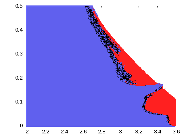
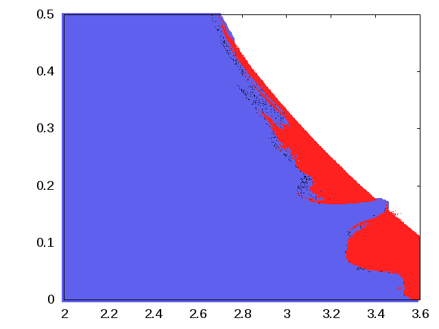
Figure 3: Parameter space of the FLM (9). The axes correspond to the parameters $\alpha$ (horizontal) and $\varepsilon$ (vertical). Candidates to SNAs are displayed (in black) for different orders ($N$) of computation, see the text for details. The values of $N$ taken for the computation (from left to right and top to bottom) are $10^{4}$, $10^{5}$, $10^{6}$ and $10^{7}$.

In this last direction we have noticed that the detection of SNAs in the parameter space using the phase sensitive operator (for a description of the method see [23]) can produce non-reliable results. In [20] it is given an example of a family of one parametric affine maps in the cylinder where the supremum norm of the derivative of the invariant curve goes to infinity when the parameter of the family tends to a certain critical value, but the invariant curve it still $C^{\infty}$ before reaching the critical value. In this case, the phase sensitive indicator will fail and it will give a false positive for parameters close to the critical value. This kind of phenomena can happen when the method is applied to the FLM giving false positives of the indicator.

To illustrate this statement we have reproduced the computation of candidates to be SNAs for the FLM done in [24]. In our computations we have considered several values of the parameter $N$ (in the notation of [23]) when computing the phase sensitivity indicator. We have fixed a box in the parameter space of the FLM, then we have discretizated it in a rectangular grid of points. For each parameter in the grid we have computed the attractor of the map and its Lyapunov exponent. In the case of having negative Lyapunov exponent we have computed the phase sensitivity indicator.

The results are shown in figure 3. The parameters values in white are the ones for which the iteration of the initial point diverged to $-\infty$. The parameters in red correspond to positive Lyapunov exponent and the ones in blue correspond to negative exponent. The points in black correspond to the candidates to be SNAs obtained with the phase sensitive indicator. The different pictures correspond to different values of the order $N$.

We can observe how the number of candidates decays when the order $N$ of the method is increased. At the end we have much less candidates that what appeared to be in the original estimations of [24]. This is due to the fact that the indicator can not distinguish between a strange set from a very wrinkled (but smooth) curve. Then when the number of iterates increases, more and more candidates to SNAs are discarded.

3.2 Parameter space and reducibility

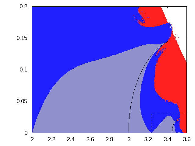
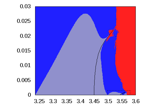
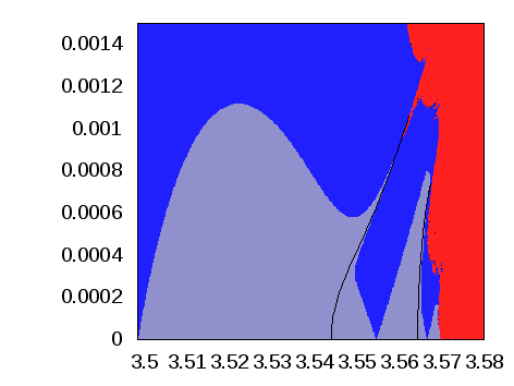
Figure 4: Diagram of the parameter space of the FLM (9) for $\omega=\frac{\sqrt{5}-1}{2}$. The axis correspond to the parameters $\alpha$ (horizontal) and $\varepsilon$ (vertical). For the correspondence of each color with the properties of the attractor see table 1.

Color		Dynamics of the attractor
Black		Invariant curve with zero Lyapunov exponent
Red		Chaotic attractor
Dark blue		Non-chaotic non-reducible attractor
Soft blue		Non-chaotic reducible attractor
White		No attractor (divergence to $-\infty$)

Table 1: Color coding for the figure 4.

As in the previous section, we consider a certain subset of the parameter space $(\alpha,\varepsilon)$ of the FLM. The parameters are classified depending on the dynamics of the attracting set, but now different properties of the attractor are considered. There are similar computations done in the literature in terms of the Lyapunov exponent of the attracting set and, in case of having a periodic invariant curve, its period ([21, 25, 9]). In our analysis, when we have an invariant periodic curve we also take into account whether the invariant curve is reducible or not. Our computation of the zero Lyapunov exponent bifurcation curve has been done approximating the invariant curve by its truncated Fourier series, instead of approximating the rotation number $\omega$ by rational approximations like in [22].

3.2.1 The procedure

We have considered three different rectangular subsets in the parameter space and we have discretized the subset in a grid of points. For each parameter in the grid we have computed the attracting set by forward iteration. Then we have computed the Lyapunov exponent of each attracting set. To compute this we have approximated the limit (7) for large values of $n$. We stopped when the variation between the estimation for $n$, $\frac{3}{4}n$ and $\frac{1}{2}n$ was lower than $10^{-3}$.

For the parameter values with negative Lyapunov exponent we assumed that we have a periodic invariant curve and we have checked if it is reducible as follows. Given a initial value $\theta_{0}\in\mathbb{T}$, we can approximate the value of the invariant curve $u$ at $\theta_{0}$ as $u(\theta_{0})\approx f^{M}(\theta_{0}-M\omega,x_{0})$ (for any $x_{0}$). This allows us to compute the attracting curve in a mesh of points. On the other hand, we have that (if $f$ is $C^{\infty}$ and $\omega$ Diophantine) an invariant curve is reducible if, and only if, $D_{x}f(\cdot,u(\cdot))$ has no zeros (see Corollary 1 of [20]). Then we can use the discrete approximation of the curve to check this condition.

The results are shown in figure 4. The parameter values where the attracting curve of the map has zero Lyapunov exponent are also displayed . In practice, this corresponds to the period doubling of the attracting invariant curve. The numerical computation of these bifurcations has been done as follows.

Given $u:\mathbb{T}\rightarrow\mathbb{R}$ an invariant curve of (3) we have that it can be approximated numerically by its truncated Fourier series at order $N$. For more details on how this can be implemented see [8, 16]. Basically, we compute the Fourier coefficients as the zero of a suitable function $G:\mathbb{R}^{2N+1}\rightarrow\mathbb{R}^{2N+1}$. For the particular case of the FLM we can add the parameters $\alpha$ and $\varepsilon$ as unknowns and extend $F$ to a function from $\mathbb{R}^{2N+3}$ to $\mathbb{R}^{2N+1}$. On the other hand, assume that we have an invariant curve which is reducible. Then we have that the Lyapunov exponent of the curve $\Lambda(u)$ given by (8) is indeed differentiable (see [20]). If we have a curve $u$ with zero Lyapunov exponent, we can use the function $\tilde{G}=(G,\Lambda)$ as a continuation function for the zero Lyapunov bifurcation curve. Then the bifurcation curve in the parameter space is computed as the projection in the $(\alpha,\varepsilon)$ coordinates of the set of zeros of $\tilde{G}$.

To compute this bifurcation curve numerically it can be used a standard continuation method (see [27]). In our case the kind of continuation that we do is rather simple. Suppose that the bifurcation curve in the parameter space is regular (no critical points). Then at every point in the parameter space the curve can be expressed locally with one of the parameters as a function of the other. When one of the parameters is fixed, the other can be computed through a standard Newton method. To do the continuation of the bifurcation curve we can vary slightly the fixed parameter and compute the corresponding value of the curve. The selection of which parameter is fixed has been done depending on the estimated inclination of the curve in the parameter space.

3.2.2 Description of the results

In figure 4 we show the results of the computation and we have also plotted two successive magnifications of certain subsets of the parameter space. These regions have been marked with a dashed line in the picture. The points in the parameter space have been codified in different colors depending on the dynamics of the attractor, see table 1.

At this point let us recall the dynamics of the logistic map. We have that for certain values of $\alpha$ the map has a cascade of period doubling bifurcations. This is, we have that there exist a sequence of values $\{d_{n}\}_{n\in\mathbb{N}}$, with $\displaystyle\lim_{n\rightarrow\infty}d_{n}=d^{*}$, such that for $\alpha\in(d_{k},d_{k+1})$ the logistic map has an attracting periodic orbit of period $2^{k}$ and at the value $\alpha=d_{k+1}$ the attractor doubles its period (from $2^{k}$ to $2^{k+1}$). Let us recall that the logistic map is unimodal for any value of $\alpha$ (i.e. it has a unique point where the derivative of the map is equal to zero). In the period doubling cascade, we also have that the attractor crosses the turning point between one period doubling and the next one. In other words, there exist values $c_{k}\in(d_{k},d_{k+1})$ for which the attracting $2^{k}$ periodic orbit of the map is the critical point.

In figure 4 we can observe that from every parameter value $(\alpha,\varepsilon)=(d_{k},0)$ it is born a curve where the attractor has zero Lyapunov exponent. Let us denote by $D_{k}$ each of these curves in the parameter space, which corresponds to the period doubling from period $2^{k}$ to $2^{k+1}$. In the bifurcation diagram at the top of figure 4 there are plotted the curves $D_{1}$ and $D_{2}$. In the bottom left one there are displayed the curves $D_{2}$ and $D_{3}$, and finally in the bottom right one there are the curves $D_{3}$ and $D_{4}$.

In the previous figure it has also been plotted the reducibility and the non-reducibility regions. We can also observe that from every parameter $c_{i}$ a “cone of non-reducibility” is born, in the sense that there exist two curves in the parameter space which define a zone where the attracting invariant curve of the map is not reducible. Let us denote by $C_{i}^{-}$ (and respectively by $C_{i}^{+}$) the left (respectively right) boundary of the non-reducibility region born at the point $c_{i}$.

We can observe how the curves $C_{i-1}^{-}$ and $C_{i}^{+}$ define an enclosed reducibility region which contains the curve $D_{i}$. Moreover these three curves seem to meet in a tangent way at the same point.

3.2.3 Analysis of the bifurcation diagram

Recall that in section 3.1 we have illustrated a truncation of the period doubling cascade for a fixed value of the coupling parameter $\varepsilon$, see figure 1. The results described above on the parameter space of the map agree with the behavior reported there. Looking at figure 4 we can observe that each period doubling is confined inside a reducibility region. Moreover, when the period is increased each of these regions get closer to the line $\varepsilon=0$. Then, if one fixes the value of $\varepsilon$ (arbitrarily small) and let $\alpha$ grow one should expect a finite number of period doublings. Fixing $\varepsilon$ at a prescribed value $\varepsilon_{0}>0$ corresponds to fixing a line $\varepsilon=\varepsilon_{0}$ in the parameter space. If the enclosed regions of reducibility get closer to $\varepsilon=0$ when the period grows, at some point the regions will be below the line $\varepsilon=\varepsilon_{0}$. On the other hand, the shape of the reducibility regions also explains why we observe a reducibility loss and afterwards a reducibility recovery between one period doubling and the next. At the same time, the bifurcation diagram displays many interesting phenomena which can be studied.

The first phenomenon that can be observed in the bifurcation diagram is the birth of non-reducibility cones around the parameters values $(\alpha,\varepsilon)=(c_{i},0)$. Recall that (definition 2.3) the reducibility loss of an invariant curve can be seen as a codimension one bifurcation. This codimension one condition defines a one dimensional curve in the parameter space, which is the boundary between the reducibility and the non-reducibility regions. With the notation introduced above, these boundaries will correspond to the curves $C_{i}^{+}$ and $C_{i}^{-}$ of the parameter space.

Actually, the existence of a cone of non-reducibility around the points $(\alpha,\varepsilon)=(c_{i},0)$ is equivalent to prove that two reducibility loss bifurcations curves are born at these points. This will be proved under suitable conditions in [18], but the phenomenon can be explained heuristically as follows.

Consider that we have an invariant (or periodic) curve $u:\mathbb{T}\rightarrow\mathbb{R}$ of the FLM. Using corollary 1 of [20] we have that $u$ is reducible if, and only if, $D_{x}f_{\alpha,\varepsilon}(\cdot,u(\cdot))$ has no zeros. For the FLM, we have that the points $(\theta,x)$ for which $D_{x}f_{\alpha,\varepsilon}(\theta,x)$ is equal to zero are those in the set $\{x=1/2\}$. Therefore an invariant curve $x=u(\theta)$ is reducible if, and only if, it does not intersect the set $x=1/2$. Respectively, a periodic curve will be reducible if, and only if, none of its periodic components touches this set.

On the other hand, when the system is uncoupled ($\varepsilon=0$) we have that the invariant (resp. periodic) curves are constant lines equal to the fixed (resp. periodic) points of the uncoupled system. For the logistic map we have that when the parameter $\alpha$ crosses the value $c_{0}$ (resp. $c_{i}$), the fixed points (resp. one of the components of the periodic orbit) crosses the set $x=1/2$. When one adds a small coupling to the system the invariant curve is no longer constant. Then when $\alpha$ is increased crossing the value $c_{0}$ (resp. $c_{i}$) the invariant curve (resp. periodic orbit) has to lose its reducibility, when it first touches $x=1/2$, and then recover it again, when it is completely below (or above) $x=1/2$. These two contacts of the invariant (or periodic) curve with the set $x=1/2$ give place to the cone of non-reducibility when the parameters $(\varepsilon,\alpha)$ are close to $(0,c_{0})$ (or $(0,c_{i})$). Each boundary of this cone correspond to a loss of reducibility bifurcation curves, namely $C_{i}^{-}$ and $C_{i}^{+}$, in the parameter space.

Another observable phenomenon in the bifurcation diagram of the figure 4 is that from every parameter value $(\alpha,\varepsilon)=(d_{i},0)$ it is born a curve in the parameter space where the attracting set has zero Lyapunov exponent. Each of these curves correspond to a period doubling bifurcation of the attractor. For diffeomorphisms it is known ([5]) that the period doubling of an invariant torus is a codimension one bifurcation. Recall that the FLM is not invertible, therefore this theory is not directly applicable. Nevertheless, in the reducible case, one can apply a normal form procedure around the invariant curve, to obtain a one dimensional system in a neighborhood of the curve. We will formalize this argument in section 5. Then we can understand the period doubling bifurcation of the invariant curve as a period doubling of the reduced system (in the classical one dimensional sense). For the uncoupled case ($\varepsilon=0$) this happens at each parameter value $\alpha=d_{i}$. Due to the codimension one character of the bifurcation a period doubling bifurcation curve is born at each of the parameters $(\alpha,\varepsilon)=(d_{i},0)$.

Figure 5: In the top left we have the invariant curve $x(\theta)$ with zero Lyapunov exponent of the FLM (9) for the terminal point of the first period doubling bifurcation. In the top right and bottom left we have the first ($x^{\prime}(\theta)$) and the second derivative ($x^{\prime\prime}(\theta)$) of the same invariant curve. In these pictures the horizontal axis corresponds to $\theta$. In the bottom right we have (in the vertical axis on a logarithmic scale) $\displaystyle\sup_{\theta\in\mathbb{T}}|x_{\varepsilon}^{\prime}(\theta)|$ (solid line) and $\displaystyle\sup_{\theta\in\mathbb{T}}|x_{\varepsilon}^{\prime\prime}(\theta)|$ (dashed line) as a graph of the parameter $\varepsilon$ (horizontal axis), where $x_{\varepsilon}$ is the invariant curve with zero Lyapunov exponent for each $\varepsilon$.

One remarkable property (observed numerically) is that each period doubling bifurcation curve $D_{i}$ is confined in a reducibility region delimited by $S_{i-1}^{+}$ and $S_{i}^{-}$. This can be explained analyzing the numerical procedure. Recall that the continuation of the bifurcation curve has been done as long as the estimated error was below a prescribed tolerance. On the other hand the function used for the numerical continuation contains the Lyapunov exponent of the invariant curve as one of its components. The method used to estimate the Lyapunov exponent behaves much worse when the reducibility is lost. Note that the Lyapunov exponent is obtained integrating numerically $\ln|D_{x}f(\theta,u(\theta))|$. In the $C^{\infty}$ case we have have that, in the reducible case the function is $C^{\infty}$ whereas in the non-reducible case the function is not even bounded. This makes the numerical integration behave much worse when the reducibility is lost. Despite of that, we have the following reasons to believe that the invariant curve (at the parameter of bifurcation) is actually destroyed due to the reducibility loss.

From the theoretical point of view, when the reducibility is lost the spectral problem associated to the continuation of the invariant curve changes drastically. When one tries to apply the IFT to an invariant curve there is a big difference from the reducible case to the non-reducible one ([20]). Given an invariant curve and its skew product consider the transfer operator associated to the curve. We have that the invariant curve can be continued when $1$ does not belongs to the spectrum of the transfer operator. In the reducible case the spectrum corresponds to the circle of radius equal to the exponential of the Lyapunov exponent of the curve. In the non-reducible case the spectrum corresponds to the disk of the same radius. When a period doubling occurs, there is an attracting invariant curve which becomes unstable, in other words its Lyapunov exponent crosses zero. In the reducible case, one might expect the spectrum of the transfer operator associated to the invariant curve (which is a circle) to cross $1$ transversally when the bifurcation happens, the curve becomes unstable but survives. But in the non-reducible case there is no chance of transversal cross.

From the numerical point of view, one can study the behavior of the invariant curve for the parameter values in the period doubling bifurcation just before losing the reducibility. In figure 5 we have displayed the invariant curve $x(\theta)$ of the FLM (9) for the parameters $(\alpha,\varepsilon)=(3.3796,0.1423)$. This parameter corresponds to the last point in the invariant curve that we have obtained in the numerical computation. In the figure we also show the first and second derivatives of the curve.

We can observe that the invariant curve $x(\theta)$ seems to keep continuous and it does not fractalize but what fractalizes is its derivative $x^{\prime}(\theta)$. Back to figure 4 we can observe that the period doubling bifurcation curve can be parameterized by the parameter $\varepsilon$. Then for each $\varepsilon$ we can consider $\alpha(\varepsilon)$ the parameter for the period doubling bifurcation curve and $x_{\varepsilon}(\theta)$ the invariant curve with zero Lyapunov exponent for the corresponding values of $\alpha$ and $\varepsilon$. In figure 5 we have the supremum of $|x^{\prime}_{\varepsilon}(\theta)|$ and $|x^{\prime\prime}_{\varepsilon}(\theta)|$ as a graph of $\varepsilon$. The figure indicates that $\displaystyle\sup_{\theta\in\mathbb{T}}|x^{\prime\prime}_{\varepsilon}(\theta)|$ grows unbounded when we approximate certain critical value $\varepsilon\approx 0.1423$. Moreover, looking at the graph of $|x^{\prime\prime}_{\varepsilon}(\theta)|$ this limit seems to be uniform when taking the supremum on any subinterval of $\mathbb{T}$.

This destruction process is similar to the fractalization process described in [20], but the curve which fractalizes here is $x^{\prime}(\theta)$. The fact that the end point of the period doubling bifurcation corresponds to the parameter where the invariant curve touches the line $x=1/2$ was already observed in [22]. The computations of the bifurcation curve done in the cited work are based on the rational approximation of the rotation number $\omega$. Our method is based on the computation of the Fourier series of the invariant curve and it has the advantage that it allow us to compute the derivatives of the curves easily.

To finish this section let us remark that this analysis is far from complete. In this direction, in the forthcoming sections 4 and 5 we present two studies in order to understand better the bifurcation diagram of the figure 4. In section 6 we summarize the different results and we analyze their implications on the cited bifurcation diagram.

4 Obstruction to reducibility

Recall that the set $x=0$ is always an invariant curve of the FLM. Apart from this set, when $\varepsilon=0$ and $\alpha>1$ we have also the invariant curve given as $x_{\alpha,0}(\theta)=1-\frac{1}{\alpha}$. Using proposition 2.6 we have that for any $\alpha\neq 3$ this curve persists for small values of $\varepsilon$. Let us denote by $x_{\alpha,\varepsilon}$ the continuation of this curve. In this section we are concerned on the reducibility of this invariant curve. Considering the images and preimages of the set of points where the derivative of the maps is equal to zero, we will construct regions in the parameter space where the curve $x_{\alpha,\varepsilon}$ can not be reducible. For instance we will see that $\alpha>2$ then $|\varepsilon|<1-\frac{1}{2}$ is a necessary condition for the reducibility of $x_{\alpha,\varepsilon}$.

In this section we will consider different sets in the cylinder $\mathbb{T}\times[0,1]$. These sets will be the closed graph of a curve or a subset of a graph. In general when we say that one of these sets is above (respectively below) of another, we mean that, for each value of $\theta\in\mathbb{T}$ the corresponding $x$-coordinate of the first set is bigger (resp. smaller) than the $x$-coordinate of the other set (for the same $\theta$). The proofs in this section have been omitted because of their simplicity.

4.1 A first constraint on the reducibility

Definition 4.1.

Given a q.p. forced map like (1), we define its critical set as the set of points on its domain where the derivative of the map (with respect to $x$) is zero. In other words,

$$P_{0}=\{(\theta,x)\in\mathbb{T}\times\mathbb{R}|\thinspace D_{x}f(\theta,x)=0\}.$$

In the case of the logistic map we have that $P_{0}=\{(\theta,x)\in\mathbb{T}\times\mathbb{R}|\thinspace x=1/2\}$.

When we have a q.p. forced map like (1) which is $C^{\infty}$ and $\omega$ is Diophantine, Corollary 1 of [20] implies that an invariant curve $y_{0}(\theta)$ is reducible if, and only if,

$$P_{0}\cap\text{Graph}(y_{0})=\emptyset,$$

where $\text{Graph}(y_{0})=\{(\theta,x)\in\mathbb{T}\times[0,1]|\thinspace x=y_{0}(\theta)\}$.

In the particular case of the FLM when $\alpha(1+|\varepsilon|)<4$ we have that the compact cylinder $\mathbb{T}\times[0,1]$ is invariant by the map. Then, any reducible invariant curve is either above or below the critical set. Actually, when the map is uncoupled ($\varepsilon=0$) we have that the invariant curve $x_{0}(\theta)=1-1/\alpha$ is above the critical set when $\alpha>2$.

Consider now $P_{1}$ the image of the critical set by the map, namely post-critical set, which is defined as

$$P_{1}=\{(\bar{\theta},\bar{x})\in\mathbb{T}\times[0,1]|\thinspace\bar{\theta}=\theta+\omega,\text{ }\bar{x}=f(\theta,x),\text{ for some }(\theta,x)\in P_{0}\}.$$

In the particular case of the FLM we have,

$$P_{1}=\left\{(\bar{\theta},\bar{x})\in\mathbb{T}\times[0,1]|\thinspace\bar{x}=\frac{\alpha}{4}(1+\varepsilon\cos(2\pi(\bar{\theta}-\omega)))\right\}.$$

Proposition 4.2.

In the case of the FLM we have the following properties on the post-critical set when $|\varepsilon|<1$.

1. The set $P_{1}$ is above the image of any other point $(\theta,x)\in\mathbb{T}\times[0,1]$.

2. The points below $P_{1}$ have two preimages in $\mathbb{T}\times\mathbb{R}$, the points in $P_{1}$ have one preimage and the points above $P_{1}$ have no preimage.

Consider the invariant curve $x_{\alpha,\varepsilon}$ of the FLM introduced at the beginning of this section. When $\varepsilon=0$ and $\alpha>2$ we have that the invariant curve exists and it is above the critical set $P_{0}$. On the other hand, $x_{\alpha,\varepsilon}$ is always below $P_{1}$ due to proposition 4.2. Concretely, we have that a necessary condition for the reducibility of $x_{\alpha,\varepsilon}$ is that $P_{0}$ and $P_{1}$ do not intersect. Otherwise there is no room for the invariant curve to exist without losing its reducibility.

Then for any $\alpha>2$ it is necessary that,

$$\frac{1}{2}<\frac{\alpha}{4}(1+\varepsilon\cos(2\pi\theta))\text{ for any }\theta\in\mathbb{T},$$

which will be satisfied if, and only if,

$$|\varepsilon|<1-\frac{2}{\alpha}.$$ (10)

This gives a first constraint in the parameter space for the reducibility of the curve $x_{\alpha,\varepsilon}$. In figure 8 we have displayed this constraint together with the bifurcation diagram computed in section 3.2. We can see that the constraint is quite sharp for values of $\alpha$ close to $2$, but it becomes rapidly pessimistic for values of $\alpha$ far from $2$.

4.2 Further constraints on the region of reducibility

Figure 6: The union of the pre-critical set of the FLM for $(\alpha,\varepsilon)=(2.75,0.12)$, from top to bottom and left to right we have the union of the $k$ first pre-critical sets, for $k=1,2,3,4$. The horizontal axis corresponds to $\theta$ and the vertical one to $x$.

In this section, we consider the preimages of the critical set to give additional restrictions to the region of the parameter space where the invariant curve $x_{\alpha,\varepsilon}$ can be reducible.

Definition 4.3.

Given $F$ a q.p. forced map like (1) we define $P_{-k}$ the $k$-th pre-critical set as the $k$-th preimage of the critical set $P_{0}$. In other words,

$$P_{-k}=\{(\theta,x)\in\mathbb{T}\times\mathbb{R}|\thinspace F^{k}(\theta,x)\in C_{0}\}.$$

In figure 6 we have (in a solid line) the first four pre-critical sets for the FLM for a concrete values of the parameters. In the figure we have (in a dashed line) the post-critical set $P_{1}$. In the top left part of the figure we have displayed the sets $P_{0}$ and $P_{-1}$. Note that $P_{0}$ lays completely below the set $P_{1}$, therefore using proposition 4.2 we have that each point of $P_{0}$ has two preimages, which will belong to $\mathbb{T}\times[0,1]$. These two preimages form the set $P_{-1}$. In the top right part of the figure we have added the set $P_{-2}$ to the previous ones. The lower component of $P_{-1}$ is below $P_{1}$ (so it has two preimages), which form part of the set $P_{-2}$. The upper component of $P_{-1}$ intersects $P_{1}$. Then only some part of it has preimage in $\mathbb{T}\times[0,1]$. Indeed, the preimages form two symmetric arches around $P_{0}$. Note that the preimage of $P_{1}$ is $P_{0}$, then the preimages of the arch of $P_{-1}$ connecting two points of $P_{0}$ are two arches connecting two points of $P_{0}$.

When further preimages are considered, higher pre-critical sets are obtained. The number of components and the shape of these components depend on the relative position of the previous pre-critical set. For example in the bottom part of the figure 6 we have added the sets $P_{-3}$ (left) and $P_{-3}\cup P_{-4}$ (right). We can observe that the two arches of $P_{-2}$ around $P_{0}$ give place to two pairs of arches of $P_{-3}$, one around each component of $P_{-1}$. Some parts of the two arches of $P_{-3}$ lay below $P_{1}$, then when we consider their preimage they give place to new arches of $P_{-4}$ around $P_{0}\cup P_{-2}$.

We are considering these pre-critical sets because they suppose an obstruction to the reducibility of the invariant curve $x_{\alpha,\varepsilon}$. Assume that $y_{0}$ is an invariant curve by the map. Since its graph is invariant by the map we have that if it intersects $P_{-k}$ for some $k$ it will eventually intersect the set $P_{0}$. Therefore given an invariant curve $y_{0}$, a necessary condition for its reducibility is that

$$P_{-k}\cap\text{Graph}(y_{0})=\emptyset\quad\forall k\geq 0,$$

where $\text{Graph}(y_{0})=\{(\theta,x)\in\mathbb{T}\times\mathbb{R}|\thinspace x=y_{0}(\theta)\}$.

For example, the FLM for the values $\alpha$ and $\varepsilon$ of the figure 6 we can see that there is a component of $P_{-4}$ which connects $P_{0}$ with $P_{1}$. Then we have that it can not exists an invariant reducible curve above $P_{0}$.

We want to formalize this discussion on the obstruction to the reducibility to give additional restrictions on the reducibility of the set $x_{\alpha,\varepsilon}$ the invariant set of the FLM introduced at the beginning of this section. To do that we need to analyze with some more detail the pre-critical set. We have the following improvement of the proposition 4.2.

Proposition 4.4.

Consider the FLM with $\alpha(1+|\varepsilon|)<4$ and the post-critical set $P_{1}=\left\{(\bar{\theta},\bar{x})\in\mathbb{T}\times\mathbb{R}|\thinspace\bar{x}=\frac{\alpha}{4}(1+\varepsilon\cos(2\pi(\bar{\theta}-\omega)))\right\}$. Consider also $S_{1}$ the set of points of the compact cylinder $\mathbb{T}\times[0,1]$ which are below or in $P_{1}$, in other words

$$S_{1}=\left\{(\theta,x)\in\mathbb{T}\times[0,1]\left|\thinspace x\leq\frac{\alpha}{4}(1+\varepsilon\cos(2\pi(\bar{\theta}-\omega)))\right.\right\}.$$

Then we have that any point $(\theta,x)\in S_{1}\setminus P_{1}$ has exactly two preimages which are given by $H_{+}(\theta,x)$ and $H_{-}(\theta,x)$, where

$$\begin{array}[]{rccc}H_{\pm}:&S_{1}&\rightarrow&\mathbb{T}^{1}\times[0,1]\\ &\left(\begin{array}[]{c}\theta\\ x\end{array}\right)&\mapsto&\left(\begin{array}[]{c}\theta-\omega\\ \rule{0.0pt}{25.83325pt}\displaystyle\frac{1}{2}\mp\sqrt{\frac{1}{4}-\frac{x}{\alpha(1+\varepsilon\cos(2\pi(\theta-\omega)))}}\end{array}\right)\end{array}$$

Moreover we have that $H_{+}$ (respectively $H_{-}$) maps homeomorphically the set $S_{1}$ to the set $\mathbb{T}\times[0,1/2]$ (and respectively $\mathbb{T}\times[1/2,1]$). Finally we have that the map $H_{+}$ preserves the orientation, in the sense that, it is monotone with respect to $x$. On the flip side the map $H_{-}$ reverses orientation, i. e. it swaps relative positions (with respect to the $x$-coordinate).

Figure 7: An example for the symbolic codification of the pre-critical sets. We have the union of the pre-critical set $P_{0}$ to $P_{4}$, and the post-critical set $P_{1}$ of the $FLM$ for $(\alpha,\varepsilon)=(2.75,0.12)$. We have indicated the symbolic codes of some of the components of the pre-critical sets. The horizontal axis corresponds to $\theta$ and the vertical one to $x$.

This result can be used to describe the pre-critical set with some more detail. By construction we have that when $\alpha>2$ the constraint (10) is satisfied, consequently the set $P_{1}$ is strictly above $P_{0}$. We can apply the proposition 4.4 to obtain that the set $P_{-1}$ is composed by the union of two different sets, i. e. $P_{-1}=P(+)\cup P(-)$, where

$$P(+)=H_{+}(C_{0})\text{ and }P(-)=H_{-}(C_{0}).$$

Moreover we have that $P(+)$ is below $P_{0}$ and $P(-)$ is above it.

Now we can consider further preimages. Since $P(+)$ is below $P_{0}$ we have that it belongs to $S_{1}$ therefore its preimages are defined. Let us denote by $P(++)=H_{+}(P(+))=H_{+}\circ H_{+}(P_{0})$ and $P(+-)=H_{-}(P(+))=H_{-}\circ H_{+}(P_{0})$.

On the other hand when, we consider the preimages of $P(-)$, we can have different relative positions between $P(-)$ and $P_{1}$ depending on the parameters. It might happen that the curve $P(-)$ is completely below $P_{1}$, completely above it or that they intersect. In the case that $P(-)$ has points above $P_{1}$ we have that $H_{\pm}$ is not defined in these points, therefore the set $H_{\pm}(P(-))$ is not well defined. This can be fixed if we formally extend $H_{\pm}$ to $\mathbb{T}\times[0,1]$ as

$$H_{\pm}(\theta,x)=\left\{\begin{array}[]{ll}H_{\pm}(\theta,x)&\text{ if }(\theta,x)\in S_{1}\\ \emptyset&\text{ otherwise}.\end{array}\right.$$

With this extension we can consider the sets $P(-\pm)=H_{\pm}(P(-))$ without problems of definition. If the set $P(-)$ is completely above $P_{1}$ we will have that $P(-\pm)=\emptyset$, and if the set $P(-)$ is partially above $P_{1}$ we have that $P(-\pm)$ is the preimage of the points below $P_{1}$. With this notation we have that

$$P_{-2}=P(++)\cup P(+-)\cup P(-+)\cup P(--).$$

This symbolic codification of the different components of $P_{-2}$ has a straight forward generalization to the sets $P_{-k}$.

Proposition 4.5.

Let $\{+,-\}^{k}$ denote the Cartesian product $k$ times of the set of two elements $\{+,-\}$. Given $s=(s_{1},\dots,s_{k})\in\{+,-\}^{k}$, let us define the set $P(s)$ as

$$P(s)=H_{s_{k}}\circ H_{s_{k-1}}\circ\dots\circ H_{s_{1}}(P_{0}).$$

Then we have,

$$P_{-k}=\bigcup_{s\in\{-,+\}^{k}}P(s).$$

In figure 7 we have the four first pre-critical sets of the FLM for the parameter values $(\alpha,\varepsilon)=(2.75,0.12)$. The symbolic codification of some of the components of the pre-critical set have been indicated in the picture. The different sequences can be deduced using proposition 4.4.

Now we will see which components of the sets $P_{-k}$ can pose an obstruction to the reducibility of the invariant curve $x_{\alpha,\varepsilon}$.

Figure 8: The different constrains on the region of reducibility of the invariant curve $x_{\alpha,\varepsilon}$ together with the bifurcation diagram of section 3.2. The curve (a) corresponds to the constraint (10), the curves (b), (c), (d) are the constrains associated to the pre-critical set $P((-)^{2})$, $P((-)^{4})$ and $P((-)^{12})$ respectively.

Consider the pre-critical sets of the FLM for $\alpha>2$ and suppose that the first constraint of reducibility (10) is satisfied. Then we have that $P(-)$ is a closed curve above $P_{0}$. To construct additional constrains on the reducibility let us assume that $P(-)$ and $P_{1}$ intersect in exactly two different points. If we consider the preimages of $P(-)$ we have that $P(-+)$ is connected by an arch to $P_{0}$ and below it. On the other hand $P(--)$ is also an arch connected to $P_{0}$ but above it. Now it can happen that $P(--)$ intersects the post-critical set $P_{1}$. If such is the case then we would have that one of the component of $P_{-2}$ connects $P_{0}$ with $P_{1}$. This would imply that no invariant reducible curve can exists between $P_{0}$ and $P_{1}$.

To avoid the situation described above, one might require the set $P(--)$ (when defined) to be below the set $P_{1}$. This condition gives place to an additional constraint in the parameter space of the FLM. In figure 8 we have this constraint on the reducibility together with the first constraint and the bifurcation diagram of section 3.2.

When the set $P(--)$ exists but it stays below $P_{1}$ we can consider further preimages of the set. We have that $P(-\pm+)=H_{+}(P(-\pm))$ will be below $P_{0}$ since we have that $H_{+}$ maps $S_{1}$ homeomorphically to $\mathbb{T}\times[0,1/2]$. Then this set does not suppose an obstruction to the reducibility. On the other hand we have that $P(-\pm)$ define two arches around $C_{0}$ the critical set, then we have that $P(-\pm-)=H_{-}(P(-\pm))$ define two arches around $P(-)$. It can happen that these arches are below $P_{1}$. If this is the case we can consider again their preimages by $H_{-}$ and $H_{+}$. The preimages by $H_{+}$ will be below $P_{0}$ then they can be discarded, because they will not become an obstruction to the reducibility of $x_{\alpha,\varepsilon}$. The set $P(-+)$ is below $P_{0}$, then $P(-+-)=H_{-}(P(-+))$ will be above $P(-)$ and then $P(-+--)=H_{-}(P(-+-))$ will be below $H_{-}(P(-))=P(--)$. If $P(--)$ does not suppose an obstruction to the reducibility, neither does $P(-+--)$. Finally the set $P(----)$ will be an arch above $P_{0}\cup P(--)$, then this can intersect the set $P_{1}$ becoming an obstruction to the reducibility.

To avoid $P(----)$ being an obstruction to the reducibility one should require it to be below $P_{1}$ for any parameter value. This will be an additional constraint to the previous ones. In figure 8 we have also added this constraint.

Finally note that the argument used above can be extended to any order. Assume that we have $P((-)^{2n})$ which exists but it is not an obstruction to reducibility, where $(-)^{2n}$ represents the $2n$ times repetition of the symbol $-$. We will have that $H_{+}(P((-)^{2n}))$ can be discarded for being below $P_{0}$, and $H_{+}\circ H_{-}(P((-)^{2n}))$ can be discarded for being below the union of all the set $P((-)^{2k})$ for $k\leq n$, then the only set which can suppose an additional restriction is $H_{-}\circ H_{-}(P((-)^{2n}))=P((-)^{2(n+1)})$.

Note that the higher order conditions does not necessarily suppose an improvement of the previous ones. For example in figure 8 we have considered the additional constraints, but not until $P((-)^{12})$ we have had an improvement to the constraint given by $P((-)^{4})$.

4.3 Remarks on the constraints

We have assumed that the sets $P((-)^{k})$ for $k$ odd intersect the set $P_{1}$ in exactly $2$ points, but we actually have that this assumption can be omitted. If the curves intersect in an even number of points we have that the discussion above is still valid but considering the different arches at the same time. When they intersect in an odd number of points there is at least one point where both curves are tangent. Then the preimage of the intersection is a single point of $P_{0}$, therefore it can be omitted. On the other hand, we have only taken into account the case where an arch of $P((-)^{2k})$ intersects the set $P_{1}$ as a possible obstruction to the reducibility of the curve $x_{\alpha,\varepsilon}$ . It might also happen that an arch of the set $P((-)^{2k})$ intersects another arch of the set $P((-)^{2r-1})$ for some $k>r>0$. This can produce also an obstruction to the reducibility of the invariant curve $x_{\alpha,\varepsilon}$ as well. But this case can be omitted because, if it occurs, then we can consider the ($2r+2$)-th image of both sets by the FLM an we will have that $P((-)^{2(k-r-1)})\cap P_{1}\neq\emptyset$.

Some other properties can be deduced for the pre-critical sets. For example, if $P((-)^{k_{0}})=\emptyset$ for some $k_{0}$, then we have that $P((-)^{k})=\emptyset$ for any $k\geq k_{0}$. On the other hand we have that if $P((-)^{2k_{0}})\cap P_{1}\neq\emptyset$ for some $k_{0}$ then $P((-)^{k})\neq\emptyset$ for any $k\geq k_{0}$. Another interesting property is the fact that when the set $P((-)^{2k})$ does not intersect $P_{1}$ for any $k>0$ then we have that between them there exist an invariant compact subset in $\mathbb{T}\times[0,1]$. The set is delimited on the top by the union of the set $P_{1}$ and the sets $P((-)^{2k+1})$ for any $k>0$, and below by the unions of the set $P_{0}$ and the sets $P((-)^{2r})$ for any $r>0$. Note that any curve inside these regions will be reducible. Indeed, when this invariant subset exists we will say that the FLM has an invariant set of reducibility.

In the previous subsection the constrains on the reducibility have been given through geometric conditions on the pre-critical set. The numerical computation of the constrains has been done as follows. We have fixed a value for $\alpha$, for instance $\alpha=3.2$. Then we have localized a value of $\varepsilon$ such that $P((-)^{2k})$ exists. We know that for $\varepsilon=1-1/\alpha$ this is satisfied, but for a better numerical stability of the computation it has been convenient to consider lower values of $\varepsilon$. Once the parameters have been fixed we have looked for the points $P((-)^{2k})\cap P_{1}$, then these points have been continued in $\varepsilon$ until a tangency between the curves has been obtained. Then the tangency has been continued in the parameter space as a constraint on the reducibility. A priori, the constraints obtained do not have to be better than the previous ones, therefore only the improvements of the constraint have been kept.

Figure 9: Some remarkable sets of the FLM for $(\alpha,\varepsilon)=(3.2,0.138)$. In a solid line we have the union of the sets $P_{0}$, $P_{-1}$, $P_{-2}$, $P_{-3}$ and all the sets of the type $P((-)^{k})$ for any $k>0$ (recall that we admit $P((-)^{k})=\emptyset$. In a dashed line we have the post-critical set $P_{1}$ and in a dotted line the attracting curve of the map. The horizontal axis corresponds to $\theta$ and the vertical one to $x$.

Analyzing the results on the figure 8, one can observe that for values of $\alpha$ close to $2$, the first constraint (10) coincides with the boundary of the parameter space where the attractor is a reducible curve. When the parameter $\alpha$ gets further from $2$ the constraint is replaced by the constraint given by the set $P((-)^{2})$, later on the constraint given by the set $P((-)^{4})$ becomes optimal, and even further this one is replaced by the constraint associated to the set $P((-)^{12})$. In other words it seems that the minimum of all the possible constrains gives the optimal constrain on the reducibility of $x_{\alpha,\varepsilon}$. We think this can be due to the fact that whenever there exists an invariant set of reducibility, then the invariant curve $x_{\alpha,\varepsilon}$ remains in the set. We have only found numerical evidences for this fact. In figure 9 we have plot the attractor of the FLM together with pre-critical sets of the map. We can observe that, even though the invariant set of reducibility is very thin, the invariant curve lays completely in its interior.

Then the different constraints on the reducibility would be optimal because they give the region (in the parameter space) of existence of the invariant set of reducibility. For parameters close to $2$ the invariant set of reducibility is delimited only by $P_{0}$ and $P_{1}$. When the parameter $\alpha$ gets further from $2$, at some point in the parameter space the invariant set of reducibility gets delimited by $P_{0}\cup P((-)^{2})$ and $P_{1}\cup P(-)$. Then, from that point on, the constraint which determines the existence of the set is the tangency between $P((-)^{2})$ and $P_{1}$, what makes the minimum of both constraints the optimal one for the reducibility. When the parameter $\alpha$ gets even further from $2$ the existence of the invariant set of reducibility is determined by higher order pre-critical sets, and the one which determines the existence of the set gives the optimal constrain.

Figure 10: In the top left we have an invariant repelling curve $x(\theta)$ of the FLM (9) for $\alpha$ fixed at $3.5$ and $\varepsilon$ just before losing its reducibility (which happens for $\varepsilon\approx 0.154086$). In the top right and bottom left we have the first ($x^{\prime}(\theta)$) and the second derivative ($x^{\prime\prime}(\theta)$) of the same invariant curve. In these pictures the horizontal axis corresponds to $\theta$. In the bottom right we have (in the vertical axis on a logarithmic scale) the supremum $|x_{\varepsilon}^{\prime}(\theta)|$ (solid line) and $|x_{\varepsilon}^{\prime\prime}(\theta)|$ (dashed line) as a graph of the parameter $\varepsilon$ (horizontal axis), where $x_{\varepsilon}$ is the continuation of the invariant curve $x_{0}(\theta)=1-1/\alpha$ for $\alpha$ fixed at $3.5$.

A final remark is that the constrains obtained do not depend on the stability of the invariant curve. In other words, they are also valid after the period doubling of the attracting set. In the unstable case, it is known that the IFT can not be applied to prove the persistence of an invariant curve after the reducibility is lost (see section 3.5 of [20]). Indeed we have done numerical computations which suggest that when the invariant curve loses its reducibility it suffers a “fractalization” process. Concretely, we have continued numerically with respect to $\varepsilon$ the curve $x_{\alpha,\varepsilon}$ for $\alpha=3.5$. To compute the invariant curve, we have approximated it by its truncated Fourier series as described in section 3.2. Looking at the bifurcation diagram in figure 4 we have that this lays completely to the right of the period doubling bifurcation. In figure 10 we have displayed the invariant curve and its derivative for the last parameter $\varepsilon$ of the continuation. We can see that the curve looks quite sharp, due to big variations of its derivative. In the same figure we have $\displaystyle\sup_{\theta\in\mathbb{T}}|x_{\alpha,\varepsilon}^{\prime}(\theta)|$ and $\displaystyle\sup_{\theta\in\mathbb{T}}|x_{\alpha,\varepsilon}^{\prime\prime}(\theta)|$ against $\varepsilon$. We can observe that that $\displaystyle\sup_{\theta\in\mathbb{T}}|x_{\alpha,\varepsilon}^{\prime\prime}(\theta)|$ seems to grow unbounded when the parameters of the map get closer to the boundary of reducibility. Note that the process of destruction is the same as the one obtained when moving the parameters through the period doubling bifurcation. If an unstable curve is really destroyed when it loses its reducibility, then we would have that the constraints on the reducibility actually enclose the region of existence of the curve $x_{\alpha,\varepsilon}$ in the unstable case.

5 Period doubling and reducibility

In section 3.2 we have studied numerically the bifurcation of the FLM. Concretely we have some bifurcation diagrams of the map in figure 4. It can be observed that from each parameter value $(\alpha,\varepsilon)=(f_{i},0)$ it is born a curve of period doubling bifurcation, which is confined in a reducibility zone. Moreover, the period doubling bifurcation curve collides (in a tangent way) with the boundaries of the reducibility, giving place to a codimension two bifurcation, namely “period doubling - reducibility loss” bifurcation. In the first part of this section we will assume that we have an invariant curve and we give a result which says that this tangent collision should be expected. In the second part we will give a model map for the reducibility regions observed in the bifurcations diagram of the FLM.

5.1 Interaction between period doubling and reducibility loss bifurcations

Theorem 3.3 of [20] describes the behavior of the Lyapunov exponent $\Lambda=\Lambda(\mu)$ of a one parametric family of maps, with respect to its parameter $\mu$ close to a value $\mu_{0}$ where the reducibility is lost. Now we will present a result which have some resemblances with the cited one, but in the following result we consider a two parametric family of maps, and then we study the interaction of the period doubling and reducibility loss bifurcations in the parameter plane.

Theorem 5.1.

Consider a one dimensional linear skew product

$$\left.\begin{array}[]{rcl}\bar{\theta}&=&\theta+\omega,\\ \bar{x}&=&a(\theta,\mu,\lambda)x,\end{array}\right\}$$ (11)

which depend ($C^{\infty}$-)smoothly on $\theta$ and (also ($C^{\infty}$-)smoothly) on two parameters $(\mu,\lambda)\in U$ with $U\subset\mathbb{R}^{2}$ an open set.

Suppose that there exists a regular curve in the parameter space, parameterized by $(\mu_{0}(t),\lambda_{0}(t))$ for $t\in[0,\varepsilon_{0})$, such that the skew product undergoes a loss of reducibility when we cross transversally that curve. Let $\Lambda(\mu,\lambda)$ denote the Lyapunov exponent of the invariant curve. Suppose also that $\Lambda(\mu_{0}(0),\lambda_{0}(0))=0$ and $\frac{d}{dt}\Lambda(\mu_{0}(t)),\lambda_{0}(t))_{t=0}\neq 0$.

Then there exists a curve in the reducibility zone of the parameter space, parameterized by $(\mu_{1}(t),\lambda_{1}(t))$ for $t\in[0,\varepsilon_{1})$, with a quadratic tangency with the previous curve and such that

$$\Lambda(\mu_{1}(t),\lambda_{1}(t))=0\text{ for any }t\in[0,\varepsilon_{1}).$$

Proof.

Consider a change of variables to new parameters $(\bar{\mu},\bar{\lambda})$ such that the curve $(\mu_{0}(t),\lambda_{0}(t))$ goes to the positive $\mu$ semiaxis. Then the reducibility loss occurs when $\bar{\lambda}$ crosses transversally zero, for any value for $\bar{\mu}\in[0,\bar{\varepsilon})$. We can apply the normal form near a reducibility loss (Lemma 3.5 of [20]) for any $\bar{\mu}$ when $\bar{\lambda}=0$. Then we have that there exist a change of variables such that the system (11) can be transformed to the following one

$$\left.\begin{array}[]{rcl}\bar{\theta}&=&\theta+\omega,\\ \bar{y}&=&h(\nu(\bar{\lambda}))(\nu(\bar{\lambda})+\cos(2\pi(\theta-\theta_{0}(\bar{\lambda}))))y,\end{array}\right\}$$ (12)

where $\nu(\bar{\lambda})$ is a smooth function of the parameter $\bar{\lambda}$, with

$$\nu(0) = 1,$$ (13)

$$\rule{0.0pt}{12.91663pt}\displaystyle\frac{\partial}{\partial\bar{\lambda}}\nu(0) \neq 0,$$ (14)

and $h(\nu)$ is a smooth function which never vanishes and $\theta_{0}(\bar{\lambda})$ a smooth function to $\mathbb{T}$.

Note that when applying Lemma 3.5 of [20] above, the original map depends smoothly on the parameter $\bar{\mu}$. Then the change of variables will also depend on it and so will do the function $\nu$, $h$ and $\theta_{0}$. Then we can think on these functions depending on both parameters and write $\nu=\nu_{\bar{\mu}}(\bar{\lambda})=\nu(\bar{\mu},\bar{\lambda})$, $h(\nu)=h_{\bar{\mu}}(\nu_{\bar{\mu}}(\bar{\lambda}))=h(\bar{\mu},\nu(\bar{\mu},\bar{\lambda}))$ and $\theta_{0}(\bar{\lambda})=\theta_{0}(\bar{\mu},\bar{\lambda})$.

The condition (14) must be satisfied for any $\bar{\mu}\in[0,\bar{\varepsilon})$, then $\frac{\partial}{\partial\bar{\lambda}}\nu(\bar{\mu},0)$ can not vanish. Changing $\bar{\mu}$ by $-\bar{\mu}$ if necessary, we can suppose that $\frac{\partial}{\partial\bar{\lambda}}\nu(\bar{\mu},0)$ is positive. Therefore conditions (13) and (14) can be rewritten as

$$\nu(\bar{\mu},0) = 1\text{ for any }\bar{\mu}\in[0,\bar{\varepsilon}),$$ (15)

$$\displaystyle\frac{\partial}{\partial\bar{\lambda}}\nu(\bar{\mu},0) > 0\text{ for any }\bar{\mu}\in[0,\bar{\varepsilon}).$$ (16)

Note that we are assuming that we have reducibility for $\bar{\lambda}>0$ and non-reducibility for $\bar{\lambda}<0$.

Using the formula (27) we can compute the Lyapunov exponent of the system,

$$\Lambda(\bar{\mu},\bar{\lambda}) = \displaystyle\int_{0}^{1}\ln|h(\bar{\mu},\nu(\bar{\mu},\bar{\lambda}))(\nu(\bar{\mu},\bar{\lambda})+\cos(2\pi(\theta-\theta_{0}(\bar{\mu},\bar{\lambda}))))|d\theta$$ (19)

$$= \rule{0.0pt}{21.52771pt}\displaystyle\int_{0}^{1}\ln|h(\bar{\mu},\nu(\bar{\mu},\bar{\lambda}))|d\theta+\int_{0}^{1}\ln|\nu(\bar{\mu},\bar{\lambda})+\cos(2\pi(\theta-\theta_{0}(\bar{\mu},\bar{\lambda})))|d\theta$$

$$= \rule{0.0pt}{43.05542pt}\left\{\begin{array}[]{lcr}\displaystyle\ln\left|\frac{h(\bar{\mu},\nu(\bar{\mu},\bar{\lambda}))}{2}\right|&\text{ if }&\bar{\lambda}\leq 0,\\ \rule{0.0pt}{21.52771pt}\displaystyle\ln\left|\frac{h(\bar{\mu},\nu(\bar{\mu},\bar{\lambda}))}{2}\right|+\operatorname{arccosh}|\nu(\bar{\mu},\bar{\lambda})|&\text{ if }&\bar{\lambda}\geq 0.\end{array}\right.$$

By hypothesis we have that $\frac{d}{dt}\Lambda(\mu_{0}(t)),\lambda_{0}(t))_{t=0}\neq 0$, performing the change of variables to the original parameters, we have that

$$\frac{\partial}{\partial\bar{\mu}}\Lambda(\bar{\mu},\bar{\lambda})_{(\bar{\mu},\bar{\lambda})=(0,0)}=\frac{d}{dt}\Lambda(\mu_{0}(t)),\lambda_{0}(t))_{t=0}\neq 0.$$

If we differentiate equation (19) with respect to $\bar{\mu}$ with the constraint $\bar{\lambda}=0$ we have

$$\frac{\partial}{\partial\bar{\mu}}\Lambda(\bar{\mu},0)=\frac{\frac{\partial}{\partial\bar{\mu}}(h(\bar{\mu},0))}{h(\bar{\mu},\nu(\bar{\mu},0))}=\frac{\partial_{\bar{\mu}}h(\bar{\mu},0)+\partial_{\nu}h(\nu(\bar{\mu},0))\cdot\partial_{\bar{\mu}}\nu(\bar{\mu},0)}{h(\bar{\mu},\nu(\bar{\mu},0))}.$$

Differentiating in (15) we have $\partial_{\bar{\mu}}\nu(\bar{\mu},0)=0$, then from the last two equations it follows that

$$\frac{\partial_{\bar{\mu}}h(0,\nu(0,0))}{h(0,\nu(0,0))}\neq 0.$$ (20)

Note that for $\bar{\lambda}>0$ we have that

$$\Lambda(\bar{\mu},\bar{\lambda})=0\text{ if, and only if, }|\nu(\bar{\mu},\bar{\lambda})|=\cosh\left(\ln{\frac{|h(\bar{\mu},\nu(\bar{\mu},\bar{\lambda}))|}{2}}\right).$$

As $\nu(\bar{\mu},0)=1$, by continuity we have $|\nu(\bar{\mu},\bar{\lambda})|=\nu(\bar{\mu},\bar{\lambda})$ for any $\bar{\lambda}$ small enough. But then, recall the $h(\bar{\mu},\nu(\bar{\mu},\bar{\lambda}))$ is a smooth function which never vanishes (in a neighborhood of $\bar{\lambda}=0$). Then, if we consider the function

$$\rho(\bar{\mu},\bar{\lambda}):=\nu(\bar{\mu},\bar{\lambda})-\cosh\left(\ln{\frac{|h(\bar{\mu},\nu(\bar{\mu},\bar{\lambda}))|}{2}}\right),$$ (21)

we have that it is a smooth function on the parameters $(\mu,\lambda)$ for $\bar{\mu}\in[0,\bar{\varepsilon})$ and $\bar{\lambda}$ small enough. Moreover from (19) we have that (when $\bar{\lambda}<0$) $\Lambda(\bar{\mu},\bar{\lambda})=0$ if, and only if, $\rho(\bar{\mu},\bar{\lambda})=0$.

To prove the theorem we first will apply the IFT to the function $\rho(\bar{\mu},\bar{\lambda})$, then we will check that the curve that we obtain is tangent to the set $\bar{\lambda}=0$ and finally that it belongs to the upper semi-plane $\bar{\lambda}>0$.

From equation (19) and the hypothesis $\Lambda(0,0)=0$ it follows that

$$\ln{\frac{|h(0,\nu(0,0))|}{2}}=0.$$ (22)

Therefore using (15) it follows that $\rho(0,0)=0$.

To apply the IFT we need to compute first the derivative of $\rho$ with respect to $\lambda$ and check that it is different from zero. We have

$$\frac{\partial}{\partial\bar{\lambda}}\rho(\bar{\mu},\bar{\lambda})=\partial_{\bar{\lambda}}\nu(\bar{\mu},\bar{\lambda})-\sinh\left(\ln{\frac{|h(\bar{\mu},\nu(\bar{\mu},\bar{\lambda}))|}{2}}\right)\frac{\partial_{\nu}h(\bar{\mu},\nu(\bar{\mu},\bar{\lambda}))\cdot\partial_{\bar{\lambda}}\nu(\bar{\mu},\bar{\lambda})}{h(\bar{\mu},\nu(\bar{\mu},\bar{\lambda}))}.$$

Evaluating at $(\bar{\mu},\bar{\lambda})=(0,0)$ and using (16) we have

$$\frac{\partial}{\partial\bar{\lambda}}\rho(0,0)=\partial_{\bar{\lambda}}\nu(0,0)>0.$$

Then we have that there exist an interval $[0,\bar{\varepsilon}_{1})$ and a function $\lambda:[0,\bar{\varepsilon}_{1})\rightarrow\mathbb{R}$ such that $\lambda(0)=0$ and $\Lambda(\mu,\lambda(\mu))=0$ for any $\mu\in[0,\bar{\varepsilon}_{1})$. Moreover we have that

$$\bar{\lambda}^{\prime}(\bar{\mu})=-\frac{\partial_{\bar{\mu}}\rho(\bar{\mu},\bar{\lambda}(\bar{\mu}))}{\partial_{\bar{\lambda}}\rho(\bar{\mu},\bar{\lambda}(\bar{\mu}))}.$$ (23)

To finish with the proof we only have to check that $\lambda^{\prime}(0)=0$ and $\lambda^{\prime\prime}(0)>0$. Differentiating in (21) with respect to $\mu$ we have,

$$\frac{\partial}{\partial\bar{\mu}}\rho(\bar{\mu},\bar{\lambda})=\partial_{\bar{\mu}}\nu(\bar{\mu},\bar{\lambda})-\sinh\left(\ln{\frac{|h(\bar{\mu},\nu(\bar{\mu},\bar{\lambda}))|}{2}}\right)\frac{\partial_{\bar{\mu}}h(\bar{\mu},\bar{\lambda})+\partial_{\nu}h(\bar{\mu},\nu(\bar{\mu},\bar{\lambda}))\cdot\partial_{\bar{\mu}}\nu(\bar{\mu},\bar{\lambda})}{h(\bar{\mu},\nu(\bar{\mu},\bar{\lambda}))}.$$ (24)

Using equations (16) and (22) we can evaluate the last equation at $(\bar{\mu},\bar{\lambda})=(0,0)$ and we have $\frac{\partial}{\partial\bar{\mu}}\rho(\bar{\mu},\bar{\lambda})=0$, therefore (using (23)) we have $\bar{\lambda}^{\prime}(\bar{\mu})=0$.

For the condition $\lambda^{\prime\prime}(0)>0$, differentiating on equation (23) and evaluating at $0$ (and using also $\bar{\lambda}^{\prime}(\bar{\mu})=0$) we have that

$$\bar{\lambda}^{\prime\prime}(0)=-\frac{\frac{\partial^{2}}{\partial\mu^{2}}\rho(0,0)}{\partial_{\bar{\lambda}}\rho(0,0)}.$$

Finally, from (15) we have also that $\frac{\partial^{2}}{\partial\mu^{2}}\nu(0,0)=0$, then differentiating equation (24), evaluating at $(\bar{\mu},\bar{\lambda})=(0,0)$ and simplifying all the zero terms we have

$$\frac{\partial^{2}}{\partial\mu^{2}}\rho(0,0)=-\left(\frac{\partial_{\bar{\mu}}h(0,\nu(0,0))}{h(0,\nu(0,0))}\right)^{2},$$

which is different from zero due to (20), therefore $\bar{\lambda}^{\prime\prime}(0)>0$. ∎

5.2 A model for the reducibility regions

In this section we present a two parametric skew product to model the interaction between the reducibility loss and the period doubling bifurcation We will see that this map is helpful for the understanding of the reducibility regions observed in the parameter space of the FLM.

Let us recall first the period doubling (and pitchfork) bifurcation for one dimensional maps. Consider the one dimensional map $\bar{x}=x(x^{2}-\mu)$, where $\mu$ is a parameter in the real line. It is well known that this map undergoes pitchfork bifurcation when the parameter $\mu$ crosses the value $-1$ and it undergoes a period doubling bifurcation when $\mu$ crosses the value $1$.

The model map that we propose is the following,

$$\left.\begin{array}[]{rcl}\bar{\theta}&=&\theta+\omega,\\ \bar{x}&=&x\left(x^{2}-(\mu+\lambda\cos(2\pi\theta))\right),\end{array}\right\}$$ (25)

where $\mu$ and $\lambda$ are parameters, and $\omega$ is Diophantine.

Note that when $\lambda$ is equal to zero the system uncouples and we obtain the model for the generic unfolding of the period doubling bifurcation when $\mu$ crosses $1$. Indeed the q.p. forcing has been considered in such a way that the set $x=0$, namely the trivial invariant set, is always an invariant curve of the map (for any parameter values).

The linear dynamics around this trivial invariant set is

$$\left.\begin{array}[]{rcl}\bar{\theta}&=&\theta+\omega,\\ \bar{x}&=&-(\mu+\lambda\cos(2\pi\theta)).\end{array}\right\}$$ (26)

We are in the $C^{\infty}$ framework, therefore by Corollary 1 in [20] we have that the trivial invariant set is reducible if, and only if, $|\lambda|<|\mu|$. In other words, the loss of reducibility bifurcation correspond to the lines in the parameter space given by $\lambda=\pm\mu$.

On the other hand, we can compute $\Lambda=\Lambda(\mu,\lambda)$ the Lyapunov exponent of the trivial invariant curve $x=0$. Recall that,

$$\int_{0}^{1}\ln|\tau+\cos(2\pi\theta)|d\theta=\left\{\begin{array}[]{lcr}-\ln{2}&\text{ if }&|\tau|\leq 1,\\ -\ln{2}+\operatorname{arccosh}|\tau|&\text{ if }&|\tau|\geq 1,\end{array}\right.$$ (27)

and $\displaystyle\operatorname{arccosh}|\tau|=\ln\left(|\tau|+\sqrt{\tau^{2}-1}\right)$ for $|\tau|\geq 1$. Using this it is easy to check that

$$\begin{array}[]{rcl}\Lambda(\mu,\lambda)&=&\displaystyle\int_{0}^{1}\ln|\mu+\lambda\cos(2\pi\theta))|d\theta\\ &=&\rule{0.0pt}{43.05542pt}\left\{\begin{array}[]{lcr}\displaystyle\ln{\left(\frac{|\mu|+\sqrt{\mu^{2}-\lambda^{2}}}{2}\right)}&\text{ if }&|\lambda|\leq|\mu|,\\ \rule{0.0pt}{21.52771pt}\displaystyle-\ln{\left|\frac{\lambda}{2}\right|}&\text{ if }&|\lambda|\geq|\mu|,\end{array}\right.\end{array}$$

Concretely, for $|\lambda|\leq|\mu|$ we have that the skew product associated to the trivial invariant set $x=0$ is reducible to

$$\left.\begin{array}[]{rcl}\bar{\theta}&=&\theta+\omega,\\ \rule{0.0pt}{12.91663pt}\displaystyle\bar{x}&=&\displaystyle-\frac{\mu+\operatorname{sign}(\mu)\sqrt{\mu^{2}-\lambda^{2}}}{2}x.\\ \end{array}\right\}$$

Therefore, in the reducible case ($|\lambda|\leq|\mu|$) the trivial invariant set changes its stability when

$$|\mu|=1+\frac{\lambda^{2}}{4}.$$

One should expect that the map (25) has a pitchfork bifurcation when one crosses the parabola $\mu=-1-\frac{\lambda^{2}}{4}$ and respectively a period doubling bifurcation when crosses $\mu=1+\frac{\lambda^{2}}{4}$. Unfortunately this can only be proved in a small region of the reducibility zone. More concretely we have the following results.

Proposition 5.2.

The model map (25) has

• Two-periodic (continuous and non-trivial) invariant curves when $0<|\lambda|<\mu$ and $1+\frac{\lambda^{2}}{2}<\mu<\frac{3}{2}-2|\lambda|$.

• Two (continuous and non-trivial) invariant curves when $\mu<-|\lambda|<0$ and $\frac{-3}{2}+2|\lambda|<\mu<-1+\frac{\lambda^{2}}{2}$.

Figure 11: Different remarkable curves of the map (25) are displayed. In a solid line we have the change of stability of the trivial invariant set. In a dashed line the loss of reducibility of the attracting set, which is the trivial invariant set or a two periodic invariant curve. Finally we have in a dotted line the boundary of applicability of the proposition 5.2. The horizontal axis corresponds to the parameter $\mu$ and the vertical one to $\lambda$.

Proof.

We will prove only the first item of the proposition, since the other one is completely analogous.

We are interested on the two periodic invariant curves of (25). Let us denote by $f$ the function which defines the system, i.e. $f(\theta,x)=x\left(x^{2}-(\mu+\lambda\cos(2\pi\theta))\right)$. Observe that $f(\theta,-x)=-f(\theta,x)$ for any $(\theta,x)\in\mathbb{T}\times\mathbb{R}$ and any parameters values. It follows that, if $u:\mathbb{T}\rightarrow\mathbb{R}$ is an invariant curve of (25), then $-u$ also is. Moreover, given a curve $u$ (different from the trivial invariant set $u\equiv 0$) satisfying

$$u(\theta+\omega)=-f(\theta,u(\theta)),\text{ for any }\theta\in\mathbb{T},$$

we have that $u$ is a two periodic solution.

Let us consider the system

$$\left.\begin{array}[]{rcl}\bar{\theta}&=&\theta+\omega\quad,\\ \bar{x}&=&h(\theta,x),\end{array}\right\}$$ (28)

where $h(\theta,x)=-f(\theta,x)=-x\left(x^{2}-(\mu+\lambda\cos(2\pi\theta))\right)$. It is clear that an invariant curve (different from $x(\theta)\equiv 0$) for the system above is a two periodic solution of (25). We will apply theorem 4.2 of [15] to this map in order to prove the existence of periodic solutions of (25). Let us check the conditions of the theorem. We have that

$$\frac{\partial}{\partial x}h(\theta,x)=-3x^{2}+\mu+\lambda\cos(2\pi\theta).$$

When $0\leq|\lambda|<\mu$ we have that $\frac{\partial}{\partial x}h(\theta,x)>0$ for any $(\theta,x)$ such that $x^{2}<\frac{\mu+\lambda\cos(2\pi\theta)}{3}$. Concretely this condition is satisfied when $x^{2}<\frac{\mu-|\lambda|}{3}$.

On the other hand, we have that

$$\frac{\partial^{2}}{\partial x^{2}}h(\theta,x)=-6x\text{ and }\frac{\partial^{3}}{\partial x^{3}}h(\theta,x)=-6,$$

therefore

$$S_{x}h(\theta,x)=\frac{-6}{\frac{\partial}{\partial x}h(\theta,x)}-\frac{3}{2}\left(\frac{-6x}{\frac{\partial}{\partial x}h(\theta,x)}\right)^{2}.$$

Note that whenever $\frac{\partial^{2}}{\partial x^{2}}h(\theta,x)>0$ then we have that $S_{x}h(\theta,x)<0$. Finally the only hypothesis remaining to be satisfied is to find an interval $I$ such that $\mathbb{T}\times I$ is invariant by the system (28). Let us consider the interval $I=\left[-\sqrt{\frac{\mu-|\lambda|}{3}}+\delta,\sqrt{\frac{\mu-|\lambda|}{3}}-\delta\right]$, with $\delta$ an arbitrary small value yet to be defined. Note that for any point on the interval the monotonicity condition is satisfied, then it is enough to check that the interval satisfies the invariance condition. In order to have invariance of the interval we have to check that

$$\left|h\left(\theta,x\right)\right|<\sqrt{\frac{\mu-|\lambda|}{3}},$$

for any $(\theta,x)\in\mathbb{T}\times I$. Since the monotonicity condition is satisfied, it is enough to check that

$$\left|h\left(\theta,\pm\sqrt{\frac{\mu-|\lambda|}{3}}-\delta\right)\right|<\sqrt{\frac{\mu-|\lambda|}{3}}-\delta.$$

Then it follows that it is enough to have

$$\left|\frac{2\mu}{3}-\left(\frac{|\lambda|}{3}+\lambda\cos(2\pi\theta)\right)-\delta\right|<1.$$

when $\mu+2|\lambda|<\frac{3}{2}$, we have that there exists a value of $\delta$ sufficiently small such that this is satisfied for any $\theta\in\mathbb{T}$.

We are in situation of applying the theorem 4.2 of [15], we know that $u(\theta)\equiv 0$ is always a continuous invariant curve, which is contained in the set $\mathbb{T}\times I$. Moreover we know its Lyapunov exponent explicitly, therefore when this crosses zero, the theorem implies that there exist two invariant curves (with negative Lyapunov exponents) of the system (25), which correspond to periodic solutions of the system (28). Moreover the invariant curves have negative Lyapunov exponent, therefore the periodic invariant curve of the original map is attracting. ∎

To illustrate this last proposition, in figure 11 we have plotted the curve which constrains the validity of proposition 5.2.

Let us assume that in the reducible case ($|\lambda|<|\mu|$) the parabola $\mu=1+\frac{\lambda^{2}}{4}$ corresponds to a period doubling bifurcation. Note that this parabola has a tangency at the points $(\mu,\lambda)=(2,\pm 2)$ with the boundary of reducibility, as predicted by theorem 5.1. Then these points in the parameter space would correspond to the “period doubling - reducibility loss” bifurcation, since it is the point where both curves merge.

Recall that in section 3.2 we have reported how the period doubling bifurcation of the FLM were enclosed inside regions of reducibility. In the proposed model (26) for the reducibility regions it is easy to justify this behavior.

Differentiating the equation which defines the map we have that the critical region of the map is $P_{0}=\{(\theta,x)\in\mathbb{T}\times I|\thinspace 3x^{2}-(\mu+\lambda\cos(2\pi\theta))=0\}$. Following the arguments of section 4 we have that a reducible invariant (or periodic) curve of (26) can not intersect the critical set. Note that for $|\lambda|<|\mu|$ the set $P_{0}$ is composed by two closed curves in the cylinder, one in each side of the trivial invariant set. Moreover when $|\lambda|$ tends to $|\mu|$ we have that the components get closer to the trivial invariant set $x=0$.

If we assume that the parabola in the parameter space $\mu=1+\frac{\lambda^{2}}{4}$ corresponds to a period doubling bifurcation, then we have that when the trivial invariant set becomes unstable then a period two solution must be created in its neighborhood. But then, when $|\lambda|$ tends to $|\mu|$ we have that the set $C_{0}$ gets closer and closer to the trivial invariant set, therefore there is no room for the period doubled curve to be reducible. This explains why arbitrarily close to the “period doubling - reducibility loss” bifurcation parameter $(\mu,\lambda)=(2,\pm 2)$ one can observe a reducibility loss of the period two invariant curve.

In figure 11 there are shown the different bifurcation curves of the map (26). The reducibility of the period two invariant curve have been estimated numerically. Let us remark the resemblance of the region of reducibility of the attractor with the same regions of the bifurcation diagram of the FLM.

6 Summary and conclusions

We study the Forced Logistic Map as a toy model for the truncation of the period doubling cascade of invariant curves. In section 3.2 we have done a numerical analysis of the bifurcation diagram of the FLM, which is displayed in figure 4. This computation revealed that each period doubling bifurcation curve in the parameter space is confined inside a region where the attracting invariant curve is reducible. Now we can use studies done in sections 4 and 5 to review the analysis of the bifurcation diagram of the FLM done in section 3.2.

In section 4 we have done a study of the critical set, their images and their preimages. We have constructed different constrains in the parameter space for the reducibility of the invariant curve $x_{\alpha,\varepsilon}$ (which is the continuation of the invariant curve $x_{\alpha,0}(\theta)=1-1/\alpha$ for $\varepsilon>0$). We have also illustrated how the combination of all these constrains seems to be the optimal constrain for the reducibility of the invariant curve. In other words, they approximate the boundary of reducibility of the attracting set of the map. Using the notation introduced in section 3.2, we have that these constraints characterize the curve $C^{+}_{0}$. In the bifurcation diagram of the figure 4 only the properties of the stable set are reflected, but we have that the constrains are still valid after the period doubling. Actually we conjecture that these constrains give the boundary of existence of the curve $x_{\alpha,\varepsilon}$ when it is unstable.

In section 5 we have studied the interaction between the reducibility loss and the period doubling bifurcation. For the case of linear skew products we have theorem 5.1, which says that generically we can expect the period doubling bifurcation curves and the reducibility loss bifurcation curve to be tangent. The diagram of the figure 4 has been done in terms of the attracting set of the FLM. As the FLM is not a linear skew product, this theorem is not applicable. But it can be applied to the linear skew product given by the linearization of the map around the invariant curve. In the same section, we have also given a model for the interaction of the period doubling bifurcation and the reducibility loss. With this model we have seen that, if the period doubling is close to a reducibility loss, then there is an obstruction to the reducibility of the period doubled curve. This explains why the curves $C^{+}_{0}$, $D_{1}$ and $C^{-}_{1}$ meet at the same point (using again the notation of section 3.2). Moreover, theorem 5.1 gives a good explanation of why they do it in a tangent way. Finally, let us remark that the study done in section 5 does not depend on the map considered, therefore it can be extended to the rest of reducibility regions determined by $C^{+}_{i-1}$ and $C^{-}_{i}$ (and containing $D_{i}$).

Part of the study done here will be continued in [17, 18, 19]. In [17] we will propose an extension of the renormalization the theory for the case of one dimensional quasi-periodic forced maps. Using this theory we will be able to prove that the curves $C^{\pm}_{i}$ of reducibility loss bifurcation really exists (for $\varepsilon$ small enough). In [18] we will use the theory proposed in the previous one to study the asymptotic behavior of the reducibility loss bifurcations when the period goes to infinity. In the previous two articles several conjectures will be done. In [19] we will support numerically this conjectures. We will give also numerical evidences of the self-renormalizable character of the bifurcation diagram of the figure 4 when different values of the rotation number $\omega$ are considered.

References

- [1] R. A. Adomaitis, I. G. Kevrekidis, and R. de la Llave. A computer-assisted study of global dynamic transitions for a noninvertible system. Internat. J. Bifur. Chaos Appl. Sci. Engrg., 17(4):1305–1321, 2007.
- [2] L. Alsedà and S. Costa. On the definition of strange nonchaotic attractor. Fund. Math., 206:23–39, 2009.
- [3] A. Arneodo, P. H. Coullet, and E. A. Spiegel. Cascade of period doublings of tori. Phys. Lett. A, 94(1):1–6, 1983.
- [4] K. Bjerklöv. SNA’s in the quasi-periodic quadratic family. Comm. Math. Phys., 286(1):137–161, 2009.
- [5] H. W. Broer, G. B. Huitema, F. Takens, and B. L. J. Braaksma. Unfoldings and bifurcations of quasi-periodic tori. Mem. Amer. Math. Soc., 83(421):viii+175, 1990.
- [6] H. W. Broer, C. Simó, and R. Vitolo. Bifurcations and strange attractors in the Lorenz-84 climate model with seasonal forcing. Nonlinearity, 15(4):1205–1267, 2002.
- [7] H. W. Broer, C. Simó, and R. Vitolo. The Hopf-saddle-node bifurcation for fixed points of 3D-diffeomorphisms: the Arnol′d resonance web. Bull. Belg. Math. Soc. Simon Stevin, 15(5, Dynamics in perturbations):769–787, 2008.
- [8] E. Castellà and A. Jorba. On the vertical families of two-dimensional tori near the triangular points of the bicircular problem. Celestial Mech. Dynam. Astronom., 76(1):35–54, 2000.
- [9] U. Feudel, S. Kuznetsov, and A. Pikovsky. Strange nonchaotic attractors, volume 56 of World Scientific Series on Nonlinear Science. Series A: Monographs and Treatises. World Scientific Publishing Co. Pte. Ltd., Hackensack, NJ, 2006. Dynamics between order and chaos in quasiperiodically forced systems.
- [10] J. Figueras and A. Haro. Computer assisted proofs of the existence of fiberwise hyperbolic invariant tori in skew products over rotations. To appear, 2010.
- [11] V. Franceschini. Bifurcations of tori and phase locking in a dissipative system of differential equations. Physica D Nonlinear Phenomena, 6:285–304, April 1983.
- [12] A. Haro and C. Simó. To be or not to be a sna: That is the question. Available at http://www.maia.ub.es/dsg/2005/index.html, 2005.
- [13] J. F. Heagy and S. M. Hammel. The birth of strange nonchaotic attractors. Phys. D, 70(1-2):140–153, 1994.
- [14] M. W. Hirsch, C. C. Pugh, and M. Shub. Invariant manifolds. Bull. Amer. Math. Soc., 76:1015–1019, 1970.
- [15] T. H. Jaeger. Quasiperiodically forced interval maps with negative schwarzian derivative. Nonlinearity, 16(4):1239–1255, 2003.
- [16] A. Jorba. Numerical computation of the normal behaviour of invariant curves of -dimensional maps. Nonlinearity, 14(5):943–976, 2001.
- [17] A. Jorba, P. Rabassa, and J.C. Tatjer. Towards a renormalization theory for quasi-periodically forced one dimensional maps I. Existence of reducibily loss bifurcations. In preparation, 2011.
- [18] A. Jorba, P. Rabassa, and J.C. Tatjer. Towards a renormalization theory for quasi-periodically forced one dimensional maps II. Asymptotic behavior of reducibility loss bifurcations. In preparation, 2011.
- [19] A. Jorba, P. Rabassa, and J.C. Tatjer. Towards a renormalization theory for quasi-periodically forced one dimensional maps III. Numerical evidences. In preparation, 2011.
- [20] A. Jorba and J. C. Tatjer. A mechanism for the fractalization of invariant curves in quasi-periodically forced 1-D maps. Discrete Contin. Dyn. Syst. Ser. B, 10(2-3):537–567, 2008.
- [21] K. Kaneko. Doubling of torus. Progr. Theoret. Phys., 69(6):1806–1810, 1983.
- [22] S. Kuznetsov, U. Feudel, and A. Pikovsky. Renormalization group of scaling at the torus-doubling terminal point. Phys. Rev. E (3), 57(2, part A):1585–1590, 1998.
- [23] A. S. Pikovsky and U. Feudel. Characterizing strange nonchaotic attractors. Chaos, 5(1):253–260, 1995.
- [24] A. Prasad, V. Mehra, and R. Ramaskrishna. Intermittency route to strange nonchaotic attractors. Phys. Rev. Let., 79(21):4127–4130, 1997.
- [25] A. Prasad, V. Mehra, and R. Ramaskrishna. Strange nonchaotic attractors in the quasiperiodically forced logistic map. Phys. Rev. E, 57(2):1576–1584, 1998.
- [26] P. Rabassa. Contribution to the study of perturbations of low dimensional maps. PhD thesis, Universitat de Barcelona, 2010.
- [27] C. Simó. On the analytical and numerical approximation of invariant manifolds. In Les Méthodes Modernes de la Mecánique Céleste (Course given at Goutelas, France, 1989), D. Benest and C. Froeschlé (eds.), pages 285–329. Editions Frontières, Paris, 1990. Available at http://www.maia.ub.es/dsg/2004/index.html.
- [28] L. van Veen. The quasi-periodic doubling cascade in the transition to weak turbulence. Phys. D, 210(3-4):249–261, 2005.