Experimental evidence of a triadic resonance of plane inertial waves in a rotating fluid

Abstract

Plane inertial waves are generated using a wavemaker, made of oscillating stacked plates, in a rotating water tank. Using particle image velocimetry, we observe that, after a transient, the primary plane wave is subject to a subharmonic instability and excites two secondary plane waves. The measured frequencies and wavevectors of these secondary waves are in quantitative agreement with the predictions of the triadic resonance mechanism. The secondary wavevectors are found systematically more normal to the rotation axis than the primary wavevector: this feature illustrates the basic mechanism at the origin of the energy transfers towards slow, quasi two-dimensional, motions in rotating turbulence.

I Introduction

Rotating and stratified fluids support the existence of two classes of anisotropic dispersive waves, called respectively inertial and internal waves, which play a major role in the dynamics of astrophysical and geophysical flows. Greenspan1968 ; Lighthill1978 ; Pedlosky1987 These waves share a number of similar properties, such as a group velocity normal to the phase velocity. Remarkably, in both cases, the frequency of the wave selects only its direction of propagation, whereas the wavelength is selected by other physical properties of the system, such as the boundary conditions or the viscosity. Lighthill1978 ; Phillips1963 ; Gostiaux2006

Most of the previous laboratory experiments on inertial waves in rotating fluids have focused on inertial modes or wave attractors in closed containers, Fultz1959 ; McEwan1970 ; Manasseh1994 ; Maas2001 ; Duguet2005 ; Duguet2006 ; Meunier2008 whereas less attention has been paid to propagative inertial wave beams. Inertial modes and attractors are generated either from a disturbance of significant size compared to the container, Fultz1959 or more classically from global forcing. McEwan1970 ; Manasseh1994 ; Maas2001 ; Duguet2005 ; Duguet2006 ; Meunier2008 Inertial modes are also detected in the ensemble average of rotating turbulence experiments in closed containers. Bewley2007 ; Lamriben2011a On the other hand, localized propagative inertial wave beams have been investigated recently in experiments using particle image velocimetry (PIV). Messio2008 ; Cortet2010

A monochromatic internal or inertial wave of finite amplitude may become unstable with respect to a parametric subharmonic instability. Thorpe1969 ; McEwan1971 ; Benielli1998 ; Staquet2002 This instability originates from a nonlinear resonant interaction of three waves, and induces an energy transfer from the primary wave towards two secondary waves of lower frequencies. This instability has received considerable interest in the case of internal gravity waves, Staquet2002 because it is believed to provide an efficient mechanism of dissipation in the oceans, by allowing a transfer of energy from the large to the small scales. Olbers1981 ; Kunze2004 ; MacKinnon2005

Parametric instability is a generic mechanism expected for any forced oscillator. A pendulum forced at twice its natural frequency provides a classical illustration of this mechanism. Here, the “parameter” is the natural frequency of the pendulum, which is modulated in time through variations of the gravity or pendulum length. Weakly nonlinear theory shows that the energy of the excitation, at frequency $\sigma_{0}$, is transferred to the pendulum at its natural frequency $\sigma_{0}/2$, resulting in an exponential growth of the oscillation amplitude.

In the case of inertial (resp. internal) waves, the “parameter” is now the so-called Coriolis frequency $f=2\Omega$, with $\Omega$ the rotation rate (resp. the Brunt-Väisälä frequency $N$). In the presence of a primary wave of frequency $\sigma_{0}$, this “parameter” becomes locally modulated in time at frequency $\sigma_{0}$, and is hence able to excite secondary waves of lower natural frequency. However, here a continuum of frequencies can be excited, so that the frequencies $\sigma_{1}$ and $\sigma_{2}$ of the secondary waves are not necessarily half the excitation frequency, but they nevertheless have to satisfy the resonant condition $\sigma_{1}+\sigma_{2}=\sigma_{0}$. Interestingly, in the absence of dissipation, the standard pendulum-like resonance $\sigma_{1}=\sigma_{2}=\sigma_{0}/2$ is recovered both for inertial and internal waves, and the corresponding secondary waves have vanishing wavelengths. Staquet2002 Viscosity is responsible here for the lift of degeneracy, by selecting a maximum growth rate corresponding to finite wavelengths, with frequencies $\sigma_{1}$ and $\sigma_{2}$ splitted on both sides of $\sigma_{0}/2$. Koudella2006

The parametric subharmonic instability has been investigated in detail for internal gravity waves. Staquet2002 ; Koudella2006 On the other hand, this instability mechanism has received less attention in the case of pure inertial waves (i.e., in absence of stratification), probably because of the lower importance of rotation effects compared to stratification effects in most geophysical flows. It has been observed in numerical simulations of inertial modes in a periodically compressed rotating cylinder. Duguet2005 ; Duguet2006 To our knowledge, parametric instability in the simpler geometry of plane inertial waves has not been investigated so far, and is the subject of this paper. A fundamental motivation for this work is the key role played by triadic interactions of inertial waves in the problem of the generation of slow quasi-2D flows in rotating turbulence. Smith1999 ; Cambon2008 ; Lamriben2011b The parametric subharmonic instability indeed provides a simple but nontrivial mechanism for anisotropic energy transfers from modes of arbitrary wavevectors towards lower frequency modes, of wavevector closer to the plane normal to the rotation axis (i.e., more “horizontal” by convention). Note that this nonlinear mechanism may however be in competition with a linear mechanism —the radiation of inertial waves along the rotation axis— which has also been shown to support the formation of vertical columnar structures.Staplehurst2008 The relative importance of these two mechanisms is governed by the Rossby number, defined as $Ro=(\tau_{\rm nl}\Omega)^{-1}$, with $\Omega^{-1}$ the linear timescale and $\tau_{\rm nl}=L/U$ the nonlinear timescale based on the characteristic velocity $U$ and length scale $L$. In rotating turbulence with $Ro\ll 1$, the anisotropy growth should hence be dominated by the nonlinear triadic interactions, whereas for $Ro=O(1)$ both mechanisms should be at play.

In this paper, we report the first experimental observation of the destabilization of a primary plane inertial wave and the subsequent excitation of subharmonic secondary waves. To produce a plane inertial wave of sufficient spatial extent, and hence of well-defined wavevector ${\bf k}_{0}$, we have made use of a wave generator already developed for internal waves in stratified fluids.Gostiaux2007 ; Mercier2008 ; Mercier2010 Wave beams of tunable shape and orientation can be generated with this wavemaker. We show that, after a transient, the excited plane wave undergoes a parametric subharmonic instability. This instability leads to the excitation of two secondary plane waves, with wavevectors which are systematically more “horizontal” than the primary wavevector. We show that the predictions from the resonant triadic interaction theory for inertial waves, as described by Smith and Waleffe,Smith1999 are in excellent agreement with our experimental results. In particular, the frequencies and wavenumbers of the secondary waves accurately match the expected theoretical values.

II Inertial plane wave generation

II.1 Structure of a plane inertial wave

We first briefly recall the main properties of inertial waves in a homogeneous fluid rotating at a constant rate $\Omega$. In the rotating frame, the restoring nature of the Coriolis force is responsible for the propagation of the inertial waves, for frequencies $\sigma\leq f$, where $f=2\Omega$ is the Coriolis parameter. Fluid particles excited at frequency $\sigma$ describe anticyclonic circles in a plane tilted at an angle $\theta=\cos^{-1}(\sigma/f)$ with respect to the horizontal, and the phase of this circular motion propagates perpendicularly to this tilted plane.

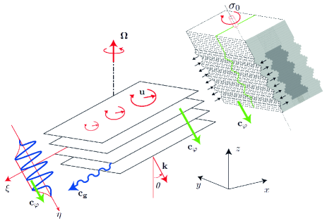
Figure 1: (Color online) Schematic representation of the wave generator. The excited plane inertial wave has a frequency $\sigma_{0}$, a downward phase velocity, a negative helicity ($s_{0}=-1$), and propagates at an angle $\theta=\cos^{-1}(\sigma_{0}/f)$, with $f=2\Omega$ the Coriolis parameter.

The equations of motion for a viscous fluid in a frame rotating at a rate $\Omega=f/2$ around the axis $z$ are

$$\partial_{t}{\bf u}+({\bf u}\cdot\nabla){\bf u} = -\frac{1}{\rho}{\bf\nabla}p-f{\bf e}_{z}\times{\bf u}+\nu\nabla^{2}{\bf u},$$ (1)

$${\bf\nabla}\bf\cdotp{\bf u} = 0,$$ (2)

where ${\bf u}=(u_{x},u_{y},u_{z})$ is the velocity field in cartesian coordinates ${\bf x}=(x,y,z)$. In the following, we restrict to the case of a flow invariant along the horizontal direction $y$. The fluid being incompressible, the motion in the vertical plane $(x,z)$ may be described by a streamfunction $\psi(x,z)$, such that ${\bf u}=(\partial_{z}\psi,u_{y},-\partial_{x}\psi)$. Neglecting viscosity, the linearized equations for small velocity disturbances are

$$\partial_{t}\partial_{z}\psi = -\frac{1}{\rho}\partial_{x}p+fu_{y},$$ (3)

$$\partial_{t}u_{y} = -f\partial_{z}\psi,$$ (4)

$$-\partial_{t}\partial_{x}\psi = -\frac{1}{\rho}\partial_{z}p.$$ (5)

These equations may be combined to obtain the equation of propagation for inertial waves,

$$\partial_{tt}(\partial_{xx}+\partial_{zz})\psi+f^{2}\partial_{zz}\psi = 0.$$ (6)

Considering a plane wave solution of frequency $\sigma$ and wavevector ${\bf k}=(k,0,m)$,

$$\psi(x,z,t)=\psi_{0}\,e^{i({\bf k}\cdot{\bf x}-\sigma t)}+{\rm c.c.}$$ (7)

(where c.c. means complex conjugate), we obtain the anisotropic dispersion relation for inertial waves

$$\sigma = sf\frac{m}{\kappa}=sf\cos\theta,$$ (8)

with $\kappa=(k^{2}+m^{2})^{1/2}$, $s=\pm 1$, and $\theta$ the angle between ${\bf k}$ and the rotation axis (see Fig. 1). We see from Eq. (8) that a given frequency $\sigma$ lower than $f$ selects a propagation angle $\pm\theta$, without specifying the norm of the wavevector $\kappa$. The corresponding velocity field is given by

$$u_{x} = im\,\psi_{0}\,e^{i(kx+mz-\sigma t)}+{\rm c.c.}$$ (9)

$$u_{y} = s\kappa\,\psi_{0}\,e^{i(kx+mz-\sigma t)}+{\rm c.c.}$$ (10)

$$u_{z} = -ik\,\psi_{0}\,e^{i(kx+mz-\sigma t)}+{\rm c.c.}$$ (11)

We recover here that the fluid particles describe anticyclonic circular motions in tilted planes perpendicular to ${\bf k}$, as sketched in Fig. 1. The wave travels with a phase velocity ${\bf c}_{\varphi}=\sigma{\bf k}/\kappa^{2}$ and a group velocity ${\bf c}_{g}=\nabla_{\bf k}\sigma$ normal to ${\bf c}_{\varphi}$. The vorticity $\boldsymbol{\omega}=\nabla\times{\bf u}$, given by

$$\boldsymbol{\omega}=-s\kappa\mathbf{u},$$ (12)

is associated to the shearing motion between planes of constant phase. Because the velocity and vorticity are aligned, inertial waves are also called helical waves, and the sign $s$ in Eq. (8) identifies to the sign of the wave helicity ${\bf u}\cdot\boldsymbol{\omega}$, with $s=+1$ for a right-handed wave and $s=-1$ for a left-handed wave. For instance, in the classical St. Andrew’s wave pattern emitted from a point source,Cortet2010 the two upper beams are right-handed and the two lower beams are left-handed, although the fluid motion is always anticyclonic.

II.2 Generation of a plane inertial wave

In order to generate a plane inertial wave, we have made use of a wavemaker, introduced by Gostiaux et al.,Gostiaux2007 which was originally designed to generate internal gravity waves (see Mercier et al.Mercier2010 for a detailed characterization of the wavemaker). This wavemaker consists in a series of oscillating stacked plates, designed to reproduce the fluid motion in the bulk of an internal gravity wave invariant along $y$. The use of this internal wave generator for the generation of inertial waves is motivated by the similarity of the spatial structure of the two types of waves in the vertical plane $(x,z)$. However, the fluid motion in the internal wave is a simple oscillating translation in the direction of the group velocity, whereas fluid particles describe anticyclonic circular translation in the case of inertial waves. As a consequence, the oscillating plates of the wavemaker only force the longitudinal component of the circular motion of the inertial waves, whereas the lateral component is let to freely adjust according to the spatial structure of the wave solution.

The wavemaker is made of a series of 48 parallelepipedic plates stacked around a helical camshaft, with the appropriate shifts between successive cames in order to form a sinusoidal profile at the surface of the generator. We introduce the local coordinate system $(\xi,y,\eta)$, tilted at an angle $\theta$ about $y$, where $\xi$ is along the wave propagation and $\eta$ is parallel to the camshaft axis (see Fig. 1). The group velocity and the phase velocity of the wave are oriented along $\xi$ and $\eta$ respectively. As the camshaft rotates at frequency $\sigma_{0}$, the plates, which are constrained in the $y$ direction, oscillate back and forth along $\xi$. The sign of the rotation of the helical camshaft selects the helicity of the excited wave, and hence an upward or downward phase velocity. In the present experiment, the rotation of the camshaft is set to produce a downward phase velocity, resulting in a left-handed inertial wave of negative helicity $s_{0}=-1$.

The cames are 14 cm wide in the $y$ direction, and their eccentricities are chosen to produce a sinusoidal displacement profile, $\xi_{0}(\eta)=\xi_{o}\,\sin(\kappa_{0}\eta)$, of wavelength $\lambda=2\pi/\kappa_{0}=7.6$ cm and amplitude $\xi_{o}=0.5$ cm at the center of the beam. The wave beam has a width 30.5 cm with a smooth decrease to 0 at the borders, and contains approximately 4 wavelengths. The generator is only forcing the $\xi$ component of the inertial wave, and the $y$ component is found to adjust according to the inertial wave structure after a distance of order of 2 cm.

The wavemaker is placed in a tank of 120 cm length, 80 cm width and 70 cm depth which is filled with 58 cm of water. The tank is mounted on the precision rotating platform “Gyroflow” of 2 m in diameter. The angular velocity $\Omega$ of the platform is set in the range 1.05 to 3.15 rad s^-1, with relative fluctuations $\Delta\Omega/\Omega$ less than $10^{-3}$. A cover is placed at the free surface, preventing from disturbances due to residual surface waves. The rotation of the fluid is set long before each experiment (at least 1 hour) in order to avoid transient spin-up recirculations and to achieve a clean solid body rotation.

The propagation angle $\theta$ of the inertial wave is varied by changing the rotation rate of the platform, while keeping the wavemaker frequency constant, $\sigma_{0}=1.05$ rad s^-1. This allows to have a fixed wave amplitude $\sigma_{0}\,\xi_{o}=0.52$ cm s^-1 for all angles. The Coriolis parameter has been varied in the range $f=1.004\,\sigma_{0}$ to $3\,\sigma_{0}$, corresponding to angles $\theta$ from 5^o to 70^o. For each value of the rotation rate, the axis of the wavemaker camshaft is tilted to the corresponding angle $\theta=\cos^{-1}(\sigma_{0}/f)$, in order to keep the plate oscillation aligned with the fluid motion in the excited wave. As a consequence, the efficiency of the forcing should not depend significantly on the angle $\theta$. For each experiment, the fluid is first reset to a solid body rotation before the wavemaker is started.

II.3 PIV measurements

Velocity fields are measured using a 2D particle image velocimetry (PIV) system Davis ; pivmat mounted on the rotating platform. The flow is seeded by 10 $\mu$m tracer particles, and illuminated by a vertical laser sheet, generated by a 140 mJ Nd:YAG pulsed laser. A vertical 59$\times$59 cm² field of view is acquired by a 14 bits 2048$\times$2048 pixels camera synchronized with the laser pulses. For each rotation rate, a set of 3200 images is recorded, at a frequency of 4 Hz, representing 24 images per wavemaker period. This frame rate is set to achieve a typical particle displacement of 5 to 10 pixels between each frame, ensuring an optimal signal-to-noise ratio for the velocity measurement. PIV computations are performed over successive images, on 32$\times$32 pixels interrogation windows with 50% overlap. The spatial resolution is 4.6 mm, which represents 17 points per wavelength of the inertial wave.

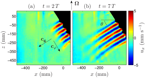
Figure 2: (Color) Horizontal velocity field after 2 and 7 periods from the start of the wavemaker for $\sigma_{0}/f=0.84$. The wavemaker is on the top-right, forcing a wave propagating along ${\bf c_{g}}$ with a phase propagating along ${\bf c_{\varphi}}$.

Figure 2 shows typical instantaneous horizontal velocity fields after 2 and 7 periods $T=2\pi/\sigma_{0}$ from the start of generator, for an experiment performed with $\sigma_{0}/f=0.84$. A well defined truncated plane wave propagates downward, making an angle $\theta=\cos^{-1}(\sigma_{0}/f)\simeq 34$^o  to the horizontal. The front of the plane wave is propagating at a velocity $8.3\pm 0.6$ mm s^-1, which agrees well with the expected group velocity $c_{g}=f\sin\theta/\kappa=8.5$ mm s^-1. The phase velocity is downward, normal to the group velocity, and also agrees with the expected value $c_{\varphi}=\sigma_{0}/\kappa=12.7$ mm s^-1.

Two sources of noise have been identified, which can be seen in the temporal energy spectrum of the velocity fields (Fig. 3, described in the next subsection): an oscillatory motion at frequency $\sigma=\Omega=0.5f$, due to a residual modulation of the rotation rate of the platform, and slowly drifting thermal convection structures at frequency $\sigma\rightarrow 0$, due to slight temperature inhomogeneities in the tank. Both effects contribute to a velocity noise of order of 0.2 mm s^-1, i.e. 25 times lower than the wave amplitude close to the wavemaker. This noise could be safely removed using a temporal Fourier filtering of the velocity fields at the forcing frequency $\sigma_{0}$. This filtering however fails in the particular case where $\sigma_{0}=\Omega$, for which the mechanical noise of the platform cannot be filtered out of the inertial wave signal.

The wavemaker is found to successfully generate well defined plane waves for frequencies $\sigma_{0}\geq 0.65f$. For lower frequency, i.e. for steeper angle of propagation [$\theta=\cos^{-1}(\sigma_{0}/f)>50$^o], the wave pattern shows significant departure from the expected plane wave profile, which may be attributed to the interference of the incident wave with the reflected wave on the bottom of the tank.

III Subharmonic Instability

III.1 Experimental observations

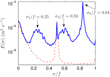
Figure 3: (Color online) Temporal energy spectra for two experiments performed at rotation rate $\Omega=0.63$ rad s^-1 with (continuous line) and without (dashed line) the wavemaker operating at $\sigma_{0}/f=0.84$. The spectrum with the generator working has been computed on the time interval between 24 and 116 periods after the start of the generator. The peak at $\sigma/f=0.5$ present in the two spectra is the trace of the mechanical noise of the platform at the rotation frequency $\sigma=\Omega$, whereas the low frequencies are due to thermal convection effects (see text).

After a few excitation periods, the front of the inertial wave has travelled outside the region of interest, and the inertial wave can be considered locally in a stationary regime. However, after typically 15 wavemaker periods (the exact value depends on the ratio $\sigma_{0}/f$), the inertial wave becomes unstable and show slow disturbances of scale slightly smaller than the excited wavelength.

We have characterized this instability using Fourier analysis of the PIV time series. We compute, at each location $(x,z)$ of the PIV field, the temporal Fourier transform of the two velocity components over a temporal window $\Delta t$,

$$\hat{\bf u}_{\sigma}(x,z)=\frac{1}{\sqrt{2\pi}}\int_{t_{0}}^{t_{0}+\Delta t}{\bf u}(x,z,t)e^{i\sigma t}dt.$$ (13)

The temporal energy spectrum is then defined as

$$E(\sigma)=\langle|\hat{\bf u}_{\sigma}|^{2}\rangle_{x,z},$$ (14)

where $\langle\cdot\rangle_{x,z}$ is the spatial average over the PIV field.

If we compute $E(\sigma)$ over a temporal window $\Delta t$ spanning a few excitation periods, we observe, as $t_{0}$ is increased, the emergence of two broad peaks at frequencies smaller than the excitation frequency $\sigma_{0}$, suggesting the growth of a subharmonic instability. These two subharmonic peaks can be seen in Fig. 3, for an experiment performed at rotation rate $\Omega=0.63$ rad s^-1 with the wavemaker operating at $\sigma_{0}/f=0.84$. Here, the temporal window $\Delta t$ is chosen equal to 92 wavemaker periods, yielding a spectral resolution of $\Delta\sigma=2\pi/\Delta t\simeq 9\times 10^{-3}\,f$. The two secondary peaks are centered on $\sigma_{1}/f=0.25\pm 0.03$ and $\sigma_{2}/f=0.59\pm 0.03$, and their sum matches well with the forcing frequency $\sigma_{0}/f=0.84$, as expected for a subharmonic resonance. The significant width of the secondary peaks, of order $0.07\,f$, indicates that this resonance is weakly selective. This broad-band selection will be further discussed in Sec. IV.2.

The subharmonic instability of the primary wave is found for all forcing frequencies $\sigma_{0}$ ranging from $0.65f$ to $f$; the measured frequencies $\sigma_{1,2}$ are given in Tab. 1. The absence of clear subharmonic instability at lower forcing frequency may be due to an intrinsic stability of the primary wave for $\sigma_{0}<0.65f$, or to the low quality of the plane wave at steep angles because of the interference with the reflected wave beam on the bottom of the tank.

$\sigma_{0}/f$	$(\sigma_{1}+\sigma_{2})/f$	$\sigma_{1}/f$	$\sigma_{2}/f$
0.64	0.64	0.19	0.45
0.71	0.71	0.21	0.50
0.84	0.84	0.25	0.59
0.91	0.94	0.27	0.67
0.95	0.97	0.29	0.68
0.98	0.98	0.32	0.66
0.99	1.00	0.34	0.66

Table 1: Frequencies of the secondary waves $\sigma_{1}/f$ and $\sigma_{2}/f$, determined from the peaks in the temporal energy spectra, as a function of the frequency of the primary wave $\sigma_{0}/f$. The uncertainty for $\sigma_{1}/f$ and $\sigma_{2}/f$ is $\pm 0.03$.

Using temporal Hilbert filtering, Mercier2008 ; Croquette1989 the spatial structure of the wave amplitude ${\bf u}_{o}({\bf x})$ and phase $\varphi({\bf x},t)={\bf k}\cdot{\bf x}-\sigma t$ can be extracted for each secondary wave. The procedure consists in (i) computing the Fourier transform $\hat{\bf u}_{\sigma}(x,z)$ of the velocity field according to Eq. (13), with a temporal window $\Delta t$ of at least 42 excitation periods; (ii) band-pass filtering $\hat{\bf u}_{\sigma}(x,z)$ around the frequency of interest $\sigma_{1}$ or $\sigma_{2}$ with a bandwidth of $\delta\sigma=2.0\,10^{-2}f$, but without including the associated negative frequency; (iii) reconstructing the complex velocity field by computing the inverse Fourier transform (including a factor 2, which accounts for the redundant negative frequency, in order to conserve energy),

$${\bf u}_{H}({\bf x},t)={\bf u}_{o}({\bf x})\,e^{i\varphi({\bf x},t)}.$$ (15)

The physical velocity field is finally given by Re$\left({\bf u}_{H}\right)$. The wave amplitude ${\bf u}_{o}$ and phase field $\varphi$ are finally obtained from the Hilbert-filtered field ${\bf u}_{H}$.

In Figs. 4(c) and (d), for the experiment at $\sigma_{0}/f=0.84$, we show the maps of the phase of the secondary waves, extracted from Hilbert filtering at frequencies $\sigma_{1}$ and $\sigma_{2}$ respectively. It is worth to note, as can be verified from Fig. 3, that the corresponding typical velocity amplitude is at least ten times smaller than for the primary wave [see Fig. 4(a)]. The spatial structures of the phase of these secondary waves are not as clearly defined as for the primary wave [Fig. 4(b)]. In particular, dislocations can be distinguished in the phase field. The finite extent of the primary wave and its spatial decay due to viscous attenuation are probably responsible for this departure of the secondary waves from pure plane waves. It is also important to note that the monochromaticity of the first subharmonic wave [Fig. 4(c)] is affected by interferences with its reflection on the wavemaker which is due to the fact this secondary wave is propagating toward the wavemaker. However, to a reasonable degree of accuracy, the two secondary waves can be considered locally as plane waves, characterized by local wavevectors ${\bf k}_{1}$ and ${\bf k}_{2}$.

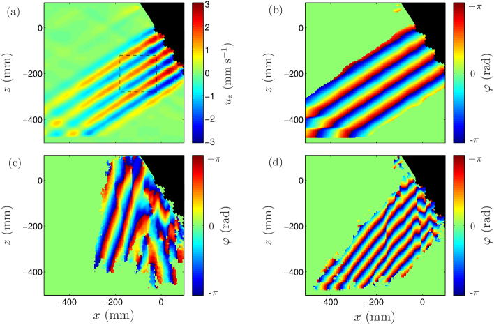
Figure 4: (Color) Hilbert filtered vertical velocity (a) and phase (b) of the primary wave at $\sigma_{0}/f=0.84$, and phase of the Hilbert filtered first [(c), $\sigma_{1}/f=0.25$] and second [(d), $\sigma_{2}/f=0.59$] subharmonic waves. The phase is displayed only where the wave amplitude is larger than $1.3\,10^{-1}\,\sigma_{0}\xi_{0}$ for (b) and $7.7\,10^{-3}\,\sigma_{0}\xi_{0}$ for (c) and (d). In (a), the square in dashed lines indicates the region where the primary wave amplitude $A_{0}$ has been measured.

III.2 Helical modes

The approximate plane wave structure of the two secondary waves suggests to analyze the instability in terms of a triadic resonance between the primary wave, of wavevector ${\bf k}_{0}$, and the two secondary waves, of wavevectors ${\bf k}_{1}$ and ${\bf k}_{2}$. This resonance may be conveniently analyzed in the framework of the helical decomposition, introduced by Waleffe, Waleffe1992 ; Waleffe1993 which we briefly recall here.

Helical modes have been introduced as a general spectral decomposition basis, which is useful to analyze the energy transfers via triadic interactions. Although this decomposition also applies for non-rotating flows, it is particularly relevant for rotating flows, because inertial plane waves have exactly the structure of helical modes. Waleffe1993 Any velocity field can actually be decomposed as a superposition of helical modes of amplitudes $A_{s_{\bf k}}({\bf k},t)$,

$${\bf u}({\bf x},t)=\sum_{\bf k}\sum_{s_{\bf k}=\pm 1}A_{s_{\bf k}}({\bf k},t)\,{\bf h}_{s_{\bf k}}({\bf k})e^{i({\bf k\cdot x}-\sigma_{s_{\bf k}}^{\bf k}t)},$$ (16)

where $\sigma_{s_{\bf k}}^{\bf k}$ is the frequency associated to a plane wave of wavevector ${\bf k}$ and helicity sign $s_{\bf k}$. The helical mode ${\bf h}_{s_{\bf k}}({\bf k})$ is normal to ${\bf k}$ (by incompressibility), and given by

$${\bf h}_{s_{\bf k}}({\bf k})=\frac{\mathbf{k}}{|\mathbf{k}|}\times\frac{\mathbf{k}\times\mathbf{e_{z}}}{|\mathbf{k}\times\mathbf{e_{z}}|}+is_{\bf k}\frac{\mathbf{k}\times\mathbf{e_{z}}}{|\mathbf{k}\times\mathbf{e_{z}}|},$$ (17)

where $s_{\bf k}=\pm 1$ is the sign of the mode helicity.fn_sign Injecting the decomposition (16) into the Navier-Stokes equation (1) yields

$$\left(\frac{\partial}{\partial t}+\nu\kappa^{2}\right)A_{\bf k}=\frac{1}{2}\sum C_{\bf kpq}^{s_{\bf k}s_{\bf p}s_{\bf q}}A^{*}_{\bf p}A^{*}_{\bf q}e^{i(\sigma_{\bf k}+\sigma_{\bf p}+\sigma_{\bf q})t},$$ (18)

with stars denoting complex conjugate, and $A_{\bf k}$, $\sigma_{\bf k}$ being short-hands for $A_{s_{\bf k}}({\bf k},t)$, $\sigma_{s_{\bf k}}^{\bf k}$. In Eq. (18), the sum is to be understood over all wavevectors ${\bf p}$ and ${\bf q}$ such that ${\bf k+p+q=0}$ and all corresponding helicity signs $s_{\bf p}$ and $s_{\bf q}$. In the following, the equation ${\bf k+p+q=0}$ will be referred to as the spatial resonance condition for a triad of helical modes. The interaction coefficient is given by

$$C_{\bf kpq}^{s_{\bf k}s_{\bf p}s_{\bf q}}=\frac{1}{2}\left[s_{\bf q}\kappa_{\bf q}-s_{\bf p}\kappa_{\bf p}\right]\left(\mathbf{h}^{*}_{s_{\bf p}}({\bf p})\times\mathbf{h}^{*}_{s_{\bf q}}({\bf q})\right)\cdot\mathbf{h}^{*}_{s_{\bf k}}({\bf k}).$$ (19)

III.3 Resonant triads

The helical mode decomposition (16) applies for any velocity field, containing an arbitrary spectrum of wavevectors. We restrict in the following the analysis to a set of three interacting inertial waves of wavevectors (${\bf k},{\bf p},{\bf q}$). Equation (18) shows that the amplitude of the mode of wavevector ${\bf k}$ is related to the two other modes ${\bf p}$ and ${\bf q}$ according to

$$\left(\frac{\partial}{\partial t}+\nu\kappa^{2}\right)A_{\bf k}=C_{\bf k}A^{*}_{\bf p}A^{*}_{\bf q}e^{i(\sigma_{\bf k}+\sigma_{\bf p}+\sigma_{\bf q})t}$$ (20)

where $C_{\bf k}$ is short-hand for $C_{\bf kpq}^{s_{\bf k}s_{\bf p}s_{\bf q}}=C_{\bf kqp}^{s_{\bf k}s_{\bf q}s_{\bf p}}$. Cyclic permutation of ${\bf k}$, ${\bf p}$ and ${\bf q}$ in Eq. (20) gives the two other relevant interaction equations between the three waves. We further restrict the analysis to plane inertial waves invariant along $y$ (i.e., $\mathbf{k}\cdot{\bf e_{y}=0}$). The three considered helical modes (17) therefore reduce to

$$\mathbf{h}_{s_{\bf r}}({\bf r})=\frac{m_{\bf r}\mathbf{e_{x}}-k_{\bf r}\mathbf{e_{z}}}{\kappa_{\bf r}}-is_{\bf r}\mathbf{e_{y}},$$ (21)

where ${\bf r}$ stands for ${\bf k}$, ${\bf p}$ or ${\bf q}$. From Eq. (21), the interaction coefficients (19) can be explicitly computed,

$$C_{\bf k}=\frac{i}{2\kappa_{\bf k}\kappa_{\bf p}\kappa_{\bf q}} \left[m_{\bf p}k_{\bf q}-m_{\bf q}k_{\bf p}\right][\kappa_{\bf q}^{2}-\kappa_{\bf p}^{2}+s_{\bf q}s_{\bf k}\kappa_{\bf q}\kappa_{\bf k}-s_{\bf p}s_{\bf k}\kappa_{\bf p}\kappa_{\bf k}],$$ (22)

and similarly for the two cyclic permutations.

Since in Eq. (20) and in its two cyclic permutations the $A_{\bf r}(t)$ coefficients have to be understood as complex velocity amplitudes evolving slowly compared to wave periods $2\pi/\sigma_{\bf r}$, temporal resonance is needed in addition to spatial resonance for the left-hand coefficients $A_{\bf r}$ to be nonzero. Using $0,1,2$ for reindexing the three waves ${\bf k}$, ${\bf p}$ and ${\bf q}$, this leads to the triadic resonance conditions

$${\bf k_{0}+k_{1}+k_{2}=0},$$ (23)

$$\sigma_{0}+\sigma_{1}+\sigma_{2}=0.$$ (24)

We consider in the following that only the primary wave $A_{0}$, of given frequency $\sigma_{0}$, wavevector ${\bf k_{0}}$ = $(k_{0},m_{0})$ and helicity sign $s_{0}$, is present initially in the system (i.e., $A_{1,2}(0)=0$). The two secondary waves ($s_{1}$, $\sigma_{1}$, ${\bf k_{1}}$) and ($s_{2}$, $\sigma_{2}$, ${\bf k_{2}}$) which could form a resonant triad with the primary wave may be determined using the resonance conditions (23) and (24). From the dispersion relation for inertial waves (8), the resonance conditions lead to

$$s_{0}\frac{m_{0}}{\sqrt{k_{0}^{2}+m_{0}^{2}}} + s_{1}\frac{m_{1}}{\sqrt{k_{1}^{2}+m_{1}^{2}}}-s_{2}\frac{m_{0}+m_{1}}{\sqrt{(k_{0}+k_{1})^{2}+(m_{0}+m_{1})^{2}}}=0.$$ (25)

For a given primary wave $(s_{0},k_{0},m_{0})$, the solution of this equation for each sign combination $(s_{0},s_{1},s_{2})$ is a curve in the $(k_{1},m_{1})$ plane (see Fig. 5). Without loss of generality, once we have taken $s_{0}=-1$ (which corresponds to the experimental configuration), it is necessary to consider four sign combinations: $(-,-,-)$, $(-,+,-)$, $(-,-,+)$ and $(-,+,+)$. Notice that the three first combinations always admit solutions, whereas the fourth one, $(-,+,+)$, admits a solution only if $|m_{0}|\leq\kappa_{0}/2$, i.e. $\theta>60$^o. The exchange of ${\bf k}_{1}$ and ${\bf k}_{2}$ keeps the $(-,-,-)$ and $(-,+,+)$ resonances unchanged, but exchanges the $(-,-,+)$ and $(-,+,-)$ resonances. Eventually, three independent sign combinations remain: $(-,-,-)$, $(-,\mp,\pm)$ and $(-,+,+)$.

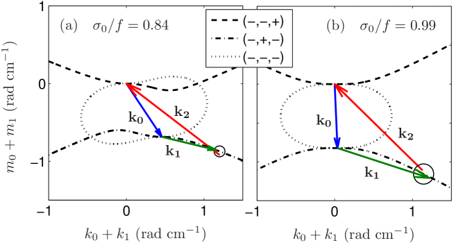
Figure 5: (Color online) Resonance curves for the primary waves (a) [$s_{0}=-1,\sigma_{0}=0.84f$, $\kappa_{0}=0.82$ rad cm^-1] and (b) [$s_{0}=-1,\sigma_{0}=0.99f$, $\kappa_{0}=0.82$ rad cm^-1]. The curves represent the location of ${\bf k}_{0}+{\bf k}_{1}=(k_{0}+k_{1},m_{0}+m_{1})$ satisfying Eq. (25) for the 3 possible combinations of signs. The wavevectors measured experimentally are shown using arrows. The circle is the theoretical prediction for the location of ${\bf k}_{0}+{\bf k}_{1}$ obtained from the maximum growth rate criterion, determined using the experimental primary wave amplitude [$A_{0}=0.29\pm 0.07$ cm s^-1 for (a) and $A_{0}=0.34\pm 0.11$ cm s^-1 for (b)]. The diameter of the circle measures the uncertainty of the prediction due to the uncertainty on the wave amplitude $A_{0}$.

III.4 Experimental verification of the resonance condition

The predictions of the triadic resonance theory are compared here with the measured wavevectors of the secondary waves. Figure 5 shows the theoretical resonance curves for two forcing frequencies, $\sigma_{0}/f=0.84$ and $0.99$. For both curves, helicity sign and wavenumber of the primary wave are chosen according to the experimental values, $s_{0}=-1$ and $\kappa_{0}=0.82$ rad cm^-1.

For both frequencies $\sigma_{0}$ considered here, only the three first sign combinations admit solutions. The $(-,-,-)$ combination gives a closed loop, whereas the two others, $(-,\mp,\pm)$, give infinite branches, tending asymptotically to constant angles. The limit of large secondary wavevectors is such that $|\sigma_{1}|=|\sigma_{2}|=|\sigma_{0}|/2$: when a wave ${\bf k}_{0}$ excites two waves of wavelength $\lambda\ll 2\pi/\kappa_{0}$, both secondary waves have frequency $\sigma_{0}/2$, with opposite wavevectors, leading to a stationary wave pattern. However, such large wavenumbers are prevented by viscosity, as will be shown in Sec. IV.1.

Figure 5 also shows the measured secondary wavevectors ${\bf k}_{1}$ and ${\bf k}_{2}$. These wavevectors are obtained from the phase fields $\varphi_{1,2}$ extracted by Hilbert filtering, using

$${\bf k}_{1,2}={\bf\nabla}\varphi_{1,2}.$$ (26)

These measurements are then averaged over regions of about (130 mm)² where the secondary waves can be considered as reasonably spatially monochromatic. It must be noted that a same plane wave can be equivalently described by ($s$, $\sigma>0$, ${\bf k}$) and ($s$, $-\sigma<0$, ${-\bf k}$). Since we always consider primary waves with positive frequency $\sigma_{0}>0$, according to Eq. (24), the subharmonic frequencies $\sigma_{1,2}$ have to be taken negative. As a consequence, the Hilbert filtering should be performed for the negative peaks in the temporal Fourier transform, in order to produce phase fields with the appropriate sign. Practically, the Hilbert filtering has been performed around the positive peaks $-\sigma_{1,2}$, and the signs of the measured wavevectors have been changed accordingly.

The secondary wavevectors ${\bf k}_{1}=(k_{1},m_{1})$ and ${\bf k}_{2}=(k_{2},m_{2})$ measured experimentally, shown in Fig. 5, are in good agreement with the triadic condition (23), forming a triangle such that ${\bf k}_{0}+{\bf k}_{1}+{\bf k}_{2}=0$. Moreover, the apex of the triangle, at ${\bf k}_{0}+{\bf k}_{1}$, falls onto one of the three resonant curves. The selected resonant curve corresponds to the sign combination $(-,+,-)$, in agreement with the observed experimental helicities. We actually verify that $s_{1}=\sigma_{1}\kappa_{1}/fm_{1}$ is positive ($\sigma_{1}<0$ and $m_{1}<0$) and that $s_{2}=\sigma_{2}\kappa_{2}/fm_{2}$ is negative ($\sigma_{2}<0$ and $m_{2}>0$), confirming the $(-,+,-)$ nature of the experimental resonance.

Interestingly, the shape of the triangle ${\bf k}_{0}+{\bf k}_{1}+{\bf k}_{2}=0$ in Fig. 5 indicates that the group velocity of the secondary wave ${\bf k}_{1}$ is oriented towards the wavemaker. Indeed, we recall that, for a given wavevector ${\bf k}$, the group velocity ${\bf c}_{g}$ is normal to ${\bf k}$, and the vertical projections of ${\bf c}_{g}$ and ${\bf k}$ are oriented in the same direction if $\sigma>0$ and in opposite directions if $\sigma<0$. Accordingly, Fig. 5 shows that ${\bf c}_{g0}$ and ${\bf c}_{g2}$ are oriented downward, pointing from the wavemaker towards the bottom of the tank, whereas ${\bf c}_{g1}$ is oriented upward, pointing towards the wavemaker. As a consequence, the secondary wave ${\bf k}_{1}$ is fed by the primary wave, but releases its energy back to the wavemaker.

For all the primary wave angles for which the instability is observed, the secondary waves are systematically such that $|\sigma_{1}|$ and $|\sigma_{2}|$ are lower than $|\sigma_{0}|$. The dispersion relation hence yields secondary wavevectors ${\bf k}_{1,2}$ more horizontal than ${\bf k}_{0}$, as illustrated in Fig. 5. This property, which actually follows from the conservation of energy and helicity,Smith1999 illustrates the natural tendency of rotating flows to transfer energy towards slow quasi-two-dimensional modes. If the process is repeated, as in rotating turbulence, the energy becomes eventually concentrated on nearly horizontal wavevectors, corresponding to a quasi-2D flow, with weak dependence along the rotation axis. Cambon2008 ; Lamriben2011b

IV Selection of the most unstable resonant triad

IV.1 Maximum growth rate criterion

In order to univocally predict the resonant secondary waves, a supplementary condition must be added to Eq. (25): we assume that the selected resonant triad is the one with the largest growth rate. Going back to the wave interaction equations (20) associated to the temporal resonance condition (24), the amplitudes of the secondary waves are governed by

$$\frac{dA_{1}}{dt}=C_{1}A^{*}_{0}A^{*}_{2}-\nu\kappa_{1}^{2}A_{1},$$ (27)

$$\frac{dA_{2}}{dt}=C_{2}A^{*}_{0}A^{*}_{1}-\nu\kappa_{2}^{2}A_{2},$$ (28)

with $C_{1,2}$ given by Eq. (22) taking ${\bf k}={\bf k}_{1,2}$ (see also Appendix A in Ref. Smith1999, ). Solving this system with initial conditions $A_{1,2}(0)=0$, and assuming that $A_{0}$ remains almost constant at short time, lead to the solutions

$$A_{1,2}(t)=B_{1,2}\,(e^{\gamma_{+}t}-e^{\gamma_{-}t}),$$ (29)

where the growth rates $\gamma_{\pm}$ write

$$\gamma_{\pm}=-\frac{\nu}{2}(\kappa_{1}^{2}+\kappa_{2}^{2})\pm\sqrt{\frac{\nu^{2}}{4}(\kappa_{1}^{2}-\kappa_{2}^{2})^{2}+C_{1}C_{2}|A_{0}|^{2}}.\quad$$ (30)

In the following, we consider the primary wave amplitude as real without loss of generality, so $|A_{0}|=A_{0}$.

The coefficient $\gamma_{-}$ is always negative, so the stability of the system is governed by the sign of $\gamma_{+}$, which we simply note $\gamma$ in the following. Interestingly, this growth rate $\gamma$ depends on the amplitude $A_{0}$ of the primary wave. As a consequence, the primary wave is unstable with respect to a given set of secondary waves, selected by the resonance condition and unequivocally denoted by $\kappa_{1}$, only if $A_{0}$ exceeds the threshold $A_{c}(\kappa_{1})=\nu\kappa_{1}\kappa_{2}/\sqrt{C_{1}C_{2}}$ in which case $\gamma(\kappa_{1})>0$. In other words, for a given couple of secondary waves (denoted by $\kappa_{1}$) to be possibly growing, the Reynolds number based on the primary wave, $Re_{0}=A_{0}/(\kappa_{0}\nu)$, must exceed a critical value $Re_{c}(\kappa_{1})=A_{c}(\kappa_{1})/(\kappa_{0}\nu)$ for the onset of the parametric instability. This critical Reynolds number is actually an increasing function of $\kappa_{1}$ and tends to zero as $\kappa_{1}\rightarrow 0$, showing that whatever the value of $Re_{0}$, there is always a continuum of resonant triads with $Re_{0}>Re_{c}(\kappa_{1})$, i.e. with a positive growth rate. The main consequence is that, whatever the value of $Re_{0}$, the most unstable triad always has a positive (maximum) growth rate and the parametric instability does not have any $Re_{0}$ threshold to proceed.

If viscosity can be neglected, Eq. (30) reduces to $\gamma=\sqrt{C_{1}C_{2}}\,A_{0}$. In the limit of large secondary wavenumbers $\kappa_{1,2}\gg\kappa_{0}$, one has ${\bf k}_{1}\simeq-{\bf k}_{2}$, and the growth rate $\gamma$ is found to tend asymptotically toward a maximum value,Koudella2006 i.e., the selected secondary waves have frequency exactly half the forcing frequency. Taking viscosity into account reduces the growth rate of the large wavenumbers, and hence selects finite wavenumbers. Equation (30) indicates that larger wavenumbers are selected for larger primary wave amplitudes $A_{0}$ and/or lower viscosity, i.e. for larger Reynolds number $Re_{0}$.

IV.2 Selection of the most unstable wavenumbers

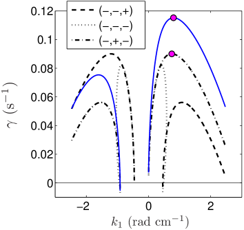
Figure 6: (Color online) Growth rates $\gamma$ as a function of $k_{1}$, computed from Eq. (30), for the three possible resonances for a primary wave $(s_{0}=-1,\sigma_{0}=0.84f$, $\kappa_{0}=0.82$ rad cm^-1). The growth rates have been computed using the average value $A_{0}=0.29$ cm s^-1 for the primary wave amplitude. For resonance $(-,+,-)$, an additional curve (continuous line) has been computed using a wave amplitude 25% larger.

In Fig. 6, the predicted growth rates $\gamma$ are plotted for the three possible sign combinations, for the primary wave defined by $s_{0}=-1,\sigma_{0}=0.84f$, $\kappa_{0}=0.82$ rad cm^-1. These growth rates have been computed using the primary wave amplitude averaged over the area where the secondary wavevectors have been measured (see the square in Fig. 4(a)), $A_{0}=0.29$ cm s^-1. For the 3 types of resonance, the growth rates tend to zero when $k_{1}\rightarrow-k_{0}/2$ and $k_{1}\rightarrow\infty$ (because of viscosity). If the secondary waves ${\bf k}_{1}$ and ${\bf k}_{2}$ are exchanged, which amounts to exchange the $(-,-,+)$ and $(-,+,-)$ resonances, the same growth rates are obtained: the curves for $(-,-,+)$ and $(-,+,-)$ are symmetrical with respect to $k_{0}/2$.

Interestingly, the growth rate is positive for a broad range of wavenumbers. Together with the broad subharmonic peaks observed in the temporal spectrum of Fig. 3, this confirms that the parametric resonance is weakly selective in this system. Values of $k_{1}$ corresponding to significant growth rates are of the same order of magnitude as the primary wavenumber $\kappa_{0}=0.82$ rad cm^-1, indicating that the viscosity has a significant effect on the selection of the excited resonant triad. For the value of $\sigma_{0}/f$ considered in Fig. 6, the maximum growth rate is obtained for the $(-,+,-)$ resonance, for $k_{1}^{\rm max}=0.75$ rad cm^-1. The corresponding predicted wavevector ${\bf k}_{1}$ is represented as a circle in the resonance curve of Fig. 5(a), and is found in excellent agreement with the experimental measurement of ${\bf k}_{1}$ (shown with an arrow).

Because of the viscous attenuation, the primary wave amplitude $A_{0}$ actually depends on the distance from the wavemaker. In the measurement area shown in Fig. 4(a), spatial variations of $\pm 25\%$ are found around the average $A_{0}=0.29$ cm s^-1. Since the growth rate (30) depends on $A_{0}$, this introduces an uncertainty on the predicted value of $\gamma$, and consequently on the selected secondary wavenumbers. In order to appreciate the influence of the measured value of $A_{0}$ on the predicted triadic resonance, we also plot in Fig. 6 the growth rate of the selected $(-,+,-)$ resonance, but for a value of $A_{0}$ increased by an amount of 25% (continuous line), which corresponds to the wave amplitude in the close vicinity of the wavemaker. The maximum growth rate is actually found to strongly depend on $A_{0}$, with an increase of 30%, indicating that the onset of the parametric instability will take place first close to the wavemaker. This strong sensitivity would make any direct comparison with an experimental growth rate too difficult. On the other hand, the selected wavenumber $k_{1}^{\rm max}$ is quite robust, showing a slight increase of 6% only when $A_{0}$ is increased by 25%. As a consequence, the uncertainty in the measurement of $A_{0}$, which is unavoidable because of the viscous attenuation of the primary wave, does not affect significantly the prediction for the most unstable secondary wavevectors.

The size of the circles in Figs. 5(a) and (b) illustrates the uncertainty in the determination of the most unstable wavevectors due to the spatial variation of $A_{0}$. The relative uncertainty lies in the range $5-15\%$ for the range of wave frequencies considered here. In spite of this uncertainty, we can conclude that the secondary wavevectors predictions from the maximum growth rate criterion are in good agreement with the observed resonant triads.

IV.3 Dependence of the secondary waves properties on the primary wave frequency

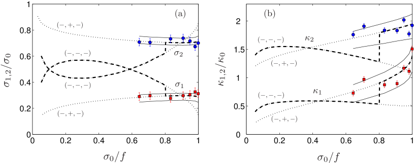
Figure 7: (Color online) Normalized frequencies $\sigma_{1,2}/\sigma_{0}$ (a), and wavenumbers $\kappa_{1,2}/\kappa_{0}$ (b) of the secondary waves, as a function of the primary wave frequency $\sigma_{0}/f$. Filled circles and squares with errorbars correspond to experimental measurements. Predictions from the triadic resonance instability are represented with dashed thick lines (using absolute maximum growth rate criterion) and dotted lines (using maximum growth rate criterion for the ($-,-,-$) and ($-,+,-$) resonances). Predictions for the most unstable resonance are ($-,-,-$) for $\sigma_{0}/f<0.79$, and ($-,+,-$) for $\sigma_{0}/f>0.79$. These predictions have been computed with a typical amplitude $A_{0}=0.30$ cm s^-1 for the primary wave. Continuous solid lines show the allowed range around the ($-,+,-$) curves, determined by considering an uncertainty of $\pm 50\%$ on $A_{0}$.

We finally characterize here the evolution of the secondary wave properties (frequencies and wavenumbers) as the frequency of the primary wave is changed. For a given primary wave amplitude $A_{0}$, the secondary frequencies $\sigma_{1,2}$ and wavenumbers $\kappa_{1,2}$ have been systematically computed according to the maximum growth rate criterion, and are reported in Fig. 7 as a function of $\sigma_{0}/f\in[0,1]$. The dotted lines correspond to the $(-,-,-)$ and $(-,+,-)$ resonances, whereas the dashed thick lines are computed from the absolute maximum growth rate among all the possible resonances. For $\sigma_{0}/f>0.79$, the growth rate is maximum on the $(-,\pm,\mp)$ branch, whereas for $\sigma_{0}/f<0.79$ it is maximum on the $(-,-,-)$ branch.

In Fig. 7, we also show the experimental measurements of $\sigma_{1,2}$ and $\kappa_{1,2}$ for the range of primary wave frequencies for which a subharmonic instability is observed, $0.65<\sigma_{0}/f<0.99$. The errorbars show the uncertainties computed from the measured frequencies and wavenumbers. The agreement with the predictions from the triadic resonance theory is excellent for the $(-,+,-)$ branch. However, it is not clear why all the measurements actually follow the $(-,+,-)$ branch, although the $(-,-,-)$ branch is expected to be more unstable for the two data points at $\sigma_{0}/f<0.79$.

The limited spatial extent of the primary wave along its transverse direction (which represents 4 wavelengths only) and its amplitude decay along its propagation direction (because of viscous attenuation) may be responsible for this unexpected stability of the $(-,-,-)$ branch at low $\sigma_{0}/f$. Indeed, the $(-,-,-)$ branch is associated to wavelengths significantly larger than the primary wavelength, so that a large spatial region of nearly homogeneous primary wave amplitude is required to sustain such large wavelength secondary waves. On the other hand, the $(-,+,-)$ resonance generates lower wavelengths, which can more easily fit into the limited extent of the primary wave. Finite size effects may therefore explain both the preferred $(-,+,-)$ resonance at $\sigma_{0}/f<0.79$, and the unexpected global stability of the primary wave for $\sigma_{0}/f<0.65$. Confinement effects are not described by the present triadic resonance theory, which assumes plane waves of infinite spatial extent. Apart from this open issue, we can conclude that, at least for sufficiently large forcing frequency, the observed secondary frequencies and wavenumbers are in good quantitative agreement with the predictions from the triadic resonance theory.

V Discussion and conclusion

Using a wavemaker initially designed to generate beams of internal gravity waves in stratified fluids, we have successfully generated well-defined plane inertial waves in a rotating water tank. Spectral analysis, performed on particle image velocimetry measurements of this plane inertial wave, has revealed the onset of a parametric instability, leading to the emergence of two secondary subharmonic waves. The wavevectors and frequencies of the primary and secondary waves are found in good agreement with the spatial and temporal resonance conditions for a resonant triad of inertial waves. Moreover, using the triadic resonance theory for inertial waves derived by Smith and Waleffe, Smith1999 the growth rate of the instability has been computed, yielding predictions for the secondary wavevectors and frequencies in agreement with the measurements. At low forcing frequency, we observe a departure from these predictions which may be associated to the finite size of the primary wave. These finite size effects cannot actually be described within the triadic resonant theory, which relies on plane waves of infinite extent.

Triadic resonant instability for inertial and internal waves share a number of common properties. In particular, equations governing the wave amplitudes equivalent to Eqs. (27) and (28) may also be derived for a triad of internal waves, but in this case, they concern the amplitude of streamfunctions and not of velocities. Koudella2006 The interaction coefficients for internal waves $\tilde{C}_{r}$ (with $r=0,1,2$) can be readily obtained from the interaction coefficients for inertial waves $C_{r}$ through a simple exchange of the vertical and horizontal components of the wavevectors, and introducing a prefactor:

$$\tilde{C}_{r}(k,m)=\frac{\kappa_{p}\kappa_{q}}{\kappa_{r}}C_{r}(m,k).$$ (31)

The $\kappa_{p}\kappa_{q}/\kappa_{r}$ prefactor between the two types of coefficients comes from the fact the wave amplitude is directly given by the velocity ${\bf u}$ in the case of inertial waves, whereas it is given by the streamfunction $\widetilde{\psi}\sim u/\kappa$ in the case of internal waves. The exchange of the vertical and horizontal components of the wavevectors comes from the comparison between the dispersion relations for inertial and internal waves, $\sigma/f=sm/\kappa$ and $\sigma/N=sk/\kappa$ respectively, with $f=2\Omega$ the Coriolis parameter and $N$ the Brunt–Väisälä frequency. The inviscid growth rate of the parametric instability $\tilde{\gamma}$ for the internal waves is actually equal to the one of inertial waves $\gamma$ through

$$\tilde{\gamma}=\sqrt{\tilde{C}_{1}\tilde{C}_{2}}\widetilde{A}_{0}=\sqrt{C_{1}C_{2}}\kappa_{0}\widetilde{A}_{0}=\gamma,$$ (32)

where $\widetilde{A}_{0}$ is the primary internal wave amplitude (homogeneous to a streamfunction). Here, the inertial wave amplitude $A_{0}$ (homogeneous to a velocity) identifies with $\kappa_{0}\widetilde{A}_{0}$. This equality between inertial and internal growth rates finally shows that the predicted secondary waves should be identical for the two types of waves.

Interacting inertial waves are of primary importance for the dynamics of rotating turbulence. In the limit of low Rossby numbers $Ro=U/\Omega L$, where $U$ and $L$ are characteristic velocity and length scales, rotating turbulence can be described as a superposition of weakly interacting inertial waves, whose interactions are directly governed by triadic resonances. This is precisely the framework of wave turbulence as analyzed in Refs. Galtier03, and Cambon04, in the context of rotating turbulence. The parametric instability between three inertial waves can be seen as an elementary process by which energy is transferred between wavevectors in rotating turbulence. This anisotropic energy transfer takes place both in scales (or wavenumbers) and directions (or angles). The angular energy transfer is always directed towards more horizontal wavevectors, providing a clear mechanism by which slow quasi-2D motions become excited.Smith1999 However, the nature of energy transfers through triadic resonance in terms of wavenumbers (or scales) —i.e., whether the energy proceeds from large to small scales or inversely— is found to depend on wave amplitude and viscosity. Indeed, it can be shown theoretically, within the present triadic resonance framework, that waves of amplitude large compared to $\nu\kappa_{0}$ are unstable with respect to secondary waves of large wavenumbers, producing a direct energy cascade towards small scales. On the other hand, waves of amplitude much lower than $\nu\kappa_{0}$ are found to excite secondary waves of smaller wavenumber, hence producing an inverse energy cascade towards larger scales. The net result of this competition is delicate to decide, and may contain an answer to the debated issue concerning the direction of the energy cascade in rapidly rotating turbulence.

- (1) H. Greenspan, “The Theory of Rotating Fluids,” (Cambridge University Press, London, 1968).
- (2) J. Lighthill, “Waves in Fluids,” (Cambridge University Press, London, 1978).
- (3) J. Pedlosky, “Geophysical Fluid Dynamics,” (Springer-Verlag, Heidelberg, 1987).
- (4) O.M. Phillips, “Energy transfer in rotating fluids by reflection of inertial waves,” Phys. Fluids 6, 513 (1963).
- (5) L. Gostiaux, T. Dauxois, H. Didelle, J. Sommeria and S. Viboud, “Quantitative laboratory observations of internal wave reflection on ascending slopes,” Phys. Fluids 18, 056602 (2006).
- (6) D. Fultz, “A note on overstability and the elastoid-inertia oscillations of Kelvin, Soldberg, and Bjerknes,” J. Meteo. 16, 199–207 (1959).
- (7) A. D. McEwan, “Inertial oscillations in a rotating fluid cylinder,” J. Fluid Mech. 40, 603–639 (1970).
- (8) R. Manasseh, “Distortions of inertia waves in a rotating fluid cylinder forced near its fundamental mode resonance,” J. Fluid Mech. 265, 345–370 (1994).
- (9) L. R. M. Maas, “Wave focusing and ensuing mean flow due to symmetry breaking in rotating fluids,” J. Fluid Mech. 437, 13–28 (2001).
- (10) Y. Duguet, J. F. Scott, L. Le Penven, “Instability inside a rotating gas cylinder subject to axial periodic strain,” Phys. Fluids 17, 114103 (2005).
- (11) Y. Duguet, J. F. Scott, L. Le Penven, “Oscillatory jets and instabilities in a rotating cylinder,” Phys. Fluids 18, 104104 (2006).
- (12) P. Meunier, C. Eloy, R. Lagrange and F. Nadal, “A rotating fluid cylinder subject to weak precession,” J. Fluid Mech. 599, 405–440 (2008).
- (13) G. P. Bewley, D. P. Lathrop, L. R. M. Maas, and K. R. Sreenivasan, “Inertial waves in rotating grid turbulence,” Phys. Fluids 19, 071701 (2007).
- (14) C. Lamriben, P.-P. Cortet, F. Moisy and L.R.M. Maas, “Excitation of inertial modes in a closed grid turbulence experiment under rotation,” Phys. Fluids 23, 015102 (2011).
- (15) L. Messio, C. Morize, M. Rabaud and F. Moisy, “Experimental observation using particle image velocimetry of inertial waves in a rotating fluid,” Exp. Fluids 44, 519-528 (2008).
- (16) P.-P. Cortet, C. Lamriben and F. Moisy, “Viscous spreading of an inertial wave beam in a rotating fluid,” Phys. Fluids 22, 086603 (2010).
- (17) S. A. Thorpe, “On standing internal gravity waves of finite amplitude,” J. Fluid Mech. 32, 489 (1969).
- (18) A. D. McEwan, “Degeneration of resonantly-excited standing internal gravity waves,” J. Fluid Mech. 50, 431 (1971).
- (19) D. Benielli and J. Sommeria, “Excitation and breaking of internal gravity waves by parametric instability,” J. Fluid Mech. 374, 117 (1998).
- (20) C. Staquet and J. Sommeria, “Internal gravity waves: From instabilities to turbulence,” Ann. Rev. Fluid Mech. 34, 559-593 (2002).
- (21) D. J. Olbers and N. Pomphrey, “Disqualifying 2 candidates for the energy-balance of oceanic internal waves,” J. Phys. Ocean. 11, 1423 (1981).
- (22) E. Kunze and S. G. Llewellyn Smith, “The Role of Small-Scale Topography in Turbulent Mixing of the Global Ocean,” Oceanography 17, 55 (2004).
- (23) J. A. MacKinnon and K. B. Winters, “Subtropical catastrophe: Significant loss of low-mode tidal energy at 28.9o,” Geophys. Res. Lett. 32, L15605 (2005).
- (24) C. R. Koudella and C. Staquet, “Instability mechanisms of a two-dimensional progressive internal gravity wave,” J. Fluid Mech. 548, 165–196 (2006).
- (25) L. M. Smith and F. Waleffe, “Transfer of energy to two-dimensional large scales in forced, rotating, three-dimensional turbulence,” Phys. Fluids 11, 1608 (1999).
- (26) P. Sagaut and C. Cambon, “Homogeneous turbulence dynamics,” Cambridge (2008).
- (27) C. Lamriben, P.-P. Cortet and F. Moisy, “Direct Measurements of Anisotropic Energy Transfers in a Rotating Turbulence Experiment,” Phys. Rev. Lett. 107, 024503 (2011).
- (28) P.J. Staplehurst, P.A. Davidson, S.B. Dalziel, “Structure formation in homogeneous freely decaying rotating turbulence,” J. Fluid Mech. 598, 81-105 (2008).
- (29) L. Gostiaux, H. Didelle, S. Mercier and T. Dauxois, “A novel internal waves generator,” Exp. Fluids 42, 123–130 (2007).
- (30) M. Mercier, N. Garnier and T. Dauxois, “Reflection and diffraction of internal waves analyzed with the Hilbert transform,” Phys. Fluids 20, 0866015 (2008).
- (31) M. Mercier, D. Martinand, M. Mathur, L. Gostiaux, T. Peacock and T. Dauxois, “New wave generation,” J. Fluid Mech. 657, 310–334 (2010).
- (32) DaVis, LaVision GmbH, Anna-Vandenhoeck-Ring 19, 37081 Goettingen, Germany.
- (33) F. Moisy, PIVMat toolbox for Matlab, http://www.fast.u-psud.fr/pivmat.
- (34) V. Croquette and H. Williams, “Nonlinear waves of the oscillatory instability on finite convective rolls,” Physica D 37, 300-314 (1989).
- (35) F. Waleffe, “The nature of triad interactions in homogeneous turbulence,” Phys. Fluids A 4 (2), 350 (1992).
- (36) F. Waleffe, “Inertial transfers in the helical decomposition,” Phys. Fluids A 5 (3), 577 (1993).
- (37) The definition of the helical mode used here corresponds to the one in Ref. Smith1999, . In Refs. Waleffe1992, and Waleffe1993, , the helical mode is defined as the complex conjugate of Eq. (17), resulting in a sign change of the helicity.
- (38) S. Galtier, “Weak inertial-wave turbulence theory,” Phys. Rev. E 68, 015301(R) (2003).
- (39) C. Cambon, R. Rubinstein, and F. S. Godeferd, “Advances in wave turbulence: rapidly rotating flows,” New J. Phys. 6, 73 (2004).