A multi-point Metropolis scheme with generic weight functions

Abstract

The multi-point Metropolis algorithm is an advanced MCMC technique based on drawing several correlated samples at each step and choosing one of them according to some normalized weights. We propose a variation of this technique where the weight functions are not specified, i.e., the analytic form can be chosen arbitrarily. This has the advantage of greater flexibility in the design of high-performance MCMC samplers. We prove that our method fulfills the balance condition, and provide a numerical simulation. We also give new insight into the functionality of different MCMC algorithms, and the connections between them.

1 Introduction

Monte Carlo statistical methods are powerful tools for numerical inference and stochastic optimization (see Robert and Casella (2004), for instance). Markov chain Monte Carlo (MCMC) methods are classical Monte Carlo techniques that generate samples from a target probability density function (pdf) by drawing from a simpler proposed pdf, usually to approximate an otherwise-incalculable (analytically) integral (Liu, 2004; Liang et al., 2010). MCMC algorithms produce a Markov chain with a stationary distribution that coincides with the target pdf.

The Metropolis-Hastings (MH) algorithm (Metropolis et al., 1953; Hastings, 1970) is the most famous MCMC technique. It can be applied to almost any target distribution. In practice, however, finding a “good” proposal pdf can be difficult. In some applications, the Markov chain generated by the MH algorithm can remain trapped almost indefinitely in a local mode meaning that, in practice, convergence may not be reached.

The Multiple-Try Metropolis (MTM) method of Liu et al. (2000) is an extension of the MH algorithm in which the next state of the chain is selected among a set of independent and identically distributed (i.i.d.) samples. This enables the MCMC sampler to make large step-size jumps without a lowering the acceptance rate; and thus MTM is can explore a larger portion of the sample space in fewer iterations.

An interesting special case of the MTM, well-known in molecular simulation field, is the orientational bias Monte Carlo, as described in Chapter 13 of Frenkel and Smit (1996) and Chapter 5 of Liu (2004), where i.i.d. candidates are drawn from a symmetric proposal pdf, and one of these is chosen according to some weights directly proportional to the target pdf. Here, however, the analytic form of the weight functions is fixed and unalterable.

Casarin et al. (2011) introduced a MTM scheme using different proposal pdfs. In this case the samples produced are independent but not identically distributed. In Qin and Liu (2001), another generalization of the MTM (called the multi-point Metropolis method) is proposed using correlated candidates at each step. Clearly, the proposal pdfs are also different in this case.

Moreover, in Pandolfi et al. (2010) an extension of the classical MTM technique is introduced where the analytic form of the weights is not specified. In Pandolfi et al. (2010), the same proposal pdf is used to draw samples, so that the candidates generated each step of the algorithm are i.i.d. Further interesting and related considerations about the use of auxiliary variables for building acceptance probabilities within a MH approach can be found in Storvik (2011).

In this paper, we draw from the two approaches (Qin and Liu, 2001) and (Pandolfi et al., 2010) to create a novel algorithm that selects a new state of the chain among correlated samples using generic weight functions, i.e., the analytic form of the weights can be chosen arbitrarily. Furthermore, we formulate the algorithm and the acceptance rule in order to fulfill the detailed balance condition.

Our method allows more flexibility in the design of efficient MCMC samplers with a larger coverage and faster exploration of the sample space. In fact, we can choose any bounded and positive weight functions to either improve performance or reduce computational complexity, independently of the chosen proposal pdf. Moreover, since in our approach the proposal pdfs are different, adaptive or interacting techniques can be applied, such as those introduced by Andrieu and Moulines (2006); Casarin et al. (2011). An important advantage of our procedure is that, since in our procedure a new candidate is drawn from a conditional pdf which depends on the samples generated earlier during the same time step, it constructs an improved proposal by automatically building on the information obtained from the generated samples.

The rest of the paper is organized as follows. In Section 2 we recall the standard multi-point Metropolis algorithm. In Section 3 we introduce our novel scheme with generic weight functions and correlated samples. Section 4 provides a rigorous proof that the novel scheme satisfies the detailed balance condition. A numerical simulation is provided in Section 5 and finally, in Section 6, we discuss the advantages of our proposed technique and provide insight into the relationships among different MTM schemes in literature.

2 Multi-point Metropolis algorithm

In the classical MH algorithm, a new possible state is drawn from the proposal pdf and the movement is accepted with a suitable decision rule. In the multi-point approach, several correlated samples are generated and, from these, a “good” one is chosen.

Specifically, consider a target pdf $p_{o}(x)$ known up to a constant (hence, we can evaluate $p(x)\propto p_{o}(x)$). Given a current state $x\in\mathbb{R}$ (we assume scalar values only for simplicity in the treatment), we draw $N$ correlated samples each step from a sequence of different proposal pdfs $\{\pi_{j}\}_{j=1}^{N}$, i.e.,

$$\begin{split}y_{1}\sim\pi_{1}(\cdot|x),&y_{2}\sim\pi_{2}(\cdot|x,y_{1}),y_{3}\sim\pi_{3}(\cdot|x,y_{1},y_{2}),\ldots\\ &\ldots y_{N}\sim\pi_{N}(\cdot|x,y_{1},...,y_{N-1}).\end{split}$$ (1)

Therefore, we can write the joint distribution of the generated samples as

$$\small q_{N}(y_{1},...,y_{N}|x)=q_{N}(y_{1:N}|x)=\pi_{1}(y_{1}|x)\pi_{2}(y_{2}|x,y_{1})\cdots\pi_{N}(y_{N}|x,y_{1:N-1}),$$ (2)

i.e.,

$$q_{N}(y_{1:N}|x)=\pi_{1}(y_{1}|x)\prod_{j=2}^{N}\pi_{j}(y_{j}|x,y_{1:j-1})$$ (3)

where, for brevity, we use the notation $y_{1:j}\triangleq[y_{1},...,y_{j}]$ and $y_{j:1}\triangleq[y_{j},...,y_{1}]$ denotes the vector with the reverse order.

A “good” candidate among the generated samples is chosen according to weight functions

$$\omega_{j}(z_{1},...,z_{j+1})\in\mathbb{R}^{j+1}\rightarrow\mathbb{R}^{+}$$

where $z_{1},...,z_{j+1}$, are generic variables and $j=1,...,N$. The specific analytic form of the weights needed in this technique is

$$\begin{split}&\omega_{j}(z_{1},...,z_{j+1})\triangleq p(z_{1})\pi_{1}(z_{2}|z_{1})\cdots\pi_{N}(z_{j}|z_{1:j-1})\lambda_{j}(z_{1},....,z_{j+1}),\end{split}$$ (4)

where $p(x)\propto p_{o}(x)$ is the target pdf, $\lambda_{j}$ can be any bounded, positive, and sequentially symmetric function, i.e.,

$$\lambda_{j}(z_{1},z_{2:j+1})=\lambda_{j}(z_{j+1:2},z_{1}).$$ (5)

Note that, since $q_{j}(z_{2:j+1}|z_{1})=\pi_{1}(z_{2}|z_{1})\cdots\pi_{N}(z_{j}|z_{1:j-1})$ (see Eq. (2)), we can rewrite the weight functions as

$$\begin{split}\omega_{j}(z_{1},...,z_{j+1})=p(z_{1})q_{j}(z_{2:j+1}|z_{1})\lambda_{j}(z_{1},z_{2:j+1}).\end{split}$$ (6)

2.1 Algorithm

Given a current state $x=x_{t}$, the multi-point Metropolis algorithm consists of the following steps:

1. Draw $N$ samples $y_{1:N}=[y_{1},y_{2},...,y_{N}]$ from the joint pdf

   $$q_{N}(y_{1:N}|x)=\pi_{1}(y_{1}|x)\prod_{j=2}^{N}\pi_{j}(y_{j}|x,y_{1:j-1})$$

   namely, draw $y_{j}$ from $\pi_{j}(\cdot|x,y_{1:j-1})$, with $j=1,...,N$.

2. Calculate the weights $\omega_{j}(y_{j:1},x)$ as in Eq. (4), and normalize them to obtain $\bar{\omega}_{j}$, $j=1,...,N$.

3. Draw a $y=y_{k}\in\{y_{1},....,y_{N}\}$ according to their weights $\bar{\omega}_{1},...,\bar{\omega}_{N}$.

4. Set

   $$x_{1}^{*}=y_{k-1},x_{2}^{*}=y_{k-2},\ldots,x_{k-1}^{*}=y_{1},$$ (7)

   and finally $x_{k}^{*}=x$. Then, draw other “reference” samples

   $$x_{j}^{*}\sim\pi_{i}(\cdot|y,x^{*}_{1:j-1}),$$ (8)

   for $j=k+1,...,N$. Note that for $j=k+1$ we have

   $$\pi_{j}(\cdot|y,x^{*}_{1:j-1})=\pi_{j}(\cdot|y,x^{*}_{1}=y_{k-1},...,x^{*}_{k-1}=y_{1},x^{*}_{k}=x),$$

   and, for $j=k+2,...,N$, we have

   $$\pi_{j}(\cdot|y,x^{*}_{1:j-1})=\pi_{j}(\cdot|y,x^{*}_{1}=y_{k-1},...,x^{*}_{k-1}=y_{1},x^{*}_{k}=x,x^{*}_{k+1:j-1}).$$

5. Compute $\omega_{j}(x_{j:1}^{*},y)$ as in Eq. (4).

6. Let $x_{t+1}=y_{k}$ with probability

   $$\alpha=\min\left[1,\frac{\sum_{j=1}^{N}\omega_{j}(y_{j:1},x)}{\sum_{j=1}^{N}\omega_{j}(x_{j:1}^{*},y)}\right],$$ (9)

   otherwise set $x_{t+1}=x$ with probability $1-\alpha$.

7. Set $t=t+1$ and repeat from step 1.

The kernel of this technique satisfies the detailed balance condition as shown in Qin and Liu (2001). However, to fulfill this condition, the algorithm needs that the weights are defined exactly with the form in Eq. (4).

3 Extension with generic weight functions

Now, we consider generic weight functions $\omega_{j}(z_{1},...,z_{j+1})\in\mathbb{R}^{j+1}\rightarrow\mathbb{R}^{+},$ that have to be (a) bounded and (b) positive. In this case, the algorithm can be described as follows.

1. Draw $N$ samples $y_{1:N}=[y_{1},y_{2},...,y_{N}]$ from the joint pdf

   $$q_{N}(y_{1:N}|x)=\pi_{1}(y_{1}|x)\prod_{j=2}^{N}\pi_{j}(y_{j}|x,y_{1:j-1})$$

   namely, draw $y_{j}$ from $\pi_{j}(\cdot|x,y_{1:j-1})$, with $j=1,...,N$.

2. Choose some suitable (bounded and positive) weight functions. Then, calculate each weight $\omega_{j}(y_{j:1},x)$, and normalize them to obtain $\bar{\omega}_{j}$, $j=1,...,N$.

3. Draw a $y=y_{k}\in\{y_{1},....,y_{N}\}$ according to $\bar{\omega}_{1},...,\bar{\omega}_{N}$, and set $\bar{W}_{y}=\bar{\omega}_{k}$, i.e.,

   $$\bar{W}_{y}\triangleq\frac{\omega_{k}(y_{k:1},x)}{\sum_{j=1}^{N}\omega_{j}(y_{j:1},x)}.$$ (10)

4. Set

   $$x_{1}^{*}=y_{k-1},x_{2}^{*}=y_{k-2},\ldots,x_{k-1}^{*}=y_{1},$$ (11)

   and finally $x_{k}^{*}=x$. Then, draw the remaining “reference” samples

   $$x_{j}^{*}\sim\pi_{j}(\cdot|y,x^{*}_{1:j-1}),$$ (12)

   for $j=k+1,...,N$.

5. Compute the general weights $\omega_{j}(x_{j:1}^{*},y)$ and calculate the normalized weight

   $$\bar{W}_{x}\triangleq\frac{\omega_{k}(x^{*}_{k:1},y)}{\sum_{j=1}^{N}\omega_{j}(x^{*}_{j:1},y)}.$$ (13)

6. Set $x_{t+1}=y_{k}$ with probability

   $$\small\alpha=\min\left[1,\frac{p(y)\pi_{1}(x^{*}_{1}|y)\pi_{2}(x^{*}_{2}|y,x^{*}_{1})\cdots\pi_{k}(x^{*}_{k}|y,x^{*}_{1},...,x^{*}_{k-1})}{p(x)\pi_{1}(y_{1}|x)\pi_{2}(y_{2}|x,y_{1})\cdots\pi_{k}(y_{k}|x,y_{1},...,y_{k-1})}\frac{\bar{W}_{x}}{\bar{W}_{y}}\right].$$ (14)

   We can rewrite it in a more compact form as

   $$\alpha=\min\left[1,\frac{p(y)q_{k}(x^{*}_{1:k}|y)}{p(x)q_{k}(y_{1:k}|x)}\frac{\bar{W}_{x}}{\bar{W}_{y}}\right],$$ (15)

   where we recall

   $$q_{k}(y_{1:k}|x)=\pi_{1}(y_{1}|x)\prod_{j=2}^{k}\pi_{j}(y_{j}|x,y_{1:j-1}).$$ (16)

   where $k$ is the index of the chosen sample $y_{k}$.
   Otherwise, set $x_{t+1}=x$ with probability $1-\alpha$.

7. Set $t=t+1$ and repeat from step 1.

We emphasise that in the algorithm above we have not specifically defined the weight functions.

3.1 Examples of weight functions

The weight functions must to be bounded and positive. The choice can depend on some criteria such as improving performance or reducing computational complexity. If the target density is bounded, two possibilities are

$$\omega_{j}(z_{1},...,z_{j+1})=p(z_{1}),$$ (17)

or

$$\omega_{j}(z_{1},...,z_{j+1})=p(z_{1})p(z_{2})\cdots p(z_{j+1}),$$ (18)

with $j=1,...,N$. Another possible choices are the following

$$\omega_{j}(z_{1},...,z_{j+1})=\left[\frac{p(z_{1})}{q_{j}(z_{1:j}|z_{j+1})}\right]^{\theta},$$ (19)

where $\theta>0$ is a positive constant, or

$$\omega_{j}(z_{1},...,z_{j+1})=\frac{p(z_{j})}{q_{1}(z_{j}|z_{j+1})}\frac{p(z_{j-1})}{q_{2}(z_{j-1:j}|z_{j+1})}\cdots\frac{p(z_{1})}{q_{j}(z_{1:j}|z_{j+1})},$$ (20)

and a third possible choice

$$\omega_{j}(z_{1},...,z_{j+1})=\frac{p(z_{1})}{\pi_{j+1}(z_{1}|z_{j+1:2})},$$ (21)

where $\pi_{j+1}(z_{1}|z_{j+1:2})$ is the $j+1$-th proposal pdf used in the step 1 of the algorithm. It is important to remark that the $z$-variables are ordered such that $z_{1}$ is the most recently generated sample, $z_{j}$ is the first drawn sample, and $z_{j+1}$ represents the previous step of the chain.

Clearly, owing to the great flexibility in the construction of the weight functions, it can be difficult to assert which is the best choice in terms of performances of the algorithm. However, evidently, in general including more statistical information in the weights can improve performance yet, at the same time, increases the computational cost of the designed technique.

More specific theoretical or empirical studies are needed to clear up this issue. Indeed, observe that the point of the best selection of the weights is even unclear in the classical MTM by Liu et al. (2000), as for the method in Pandolfi et al. (2010), for instance.

3.2 Relationship with the independent multiple tries scheme

In Pandolfi et al. (2010) i.i.d. candidates are proposed at each time step. The acceptance probability $\alpha$ in Eqs. (14)-(15) may appear similar to the acceptance probability in Pandolfi et al. (2010). However, note that the expression of $\alpha$ in Eq. (15) is different to the acceptance probability in Pandolfi et al. (2010) for two main reasons:

• the first factor $\frac{p(y)q_{k}(x^{*}_{1:k}|y)}{p(x)q_{k}(y_{1:k}|x)}$ is distinct (see Eqs. (16)), and

• the definition and computation of $\bar{W}_{x}$ and $\bar{W}_{y}$ (see Eqs. (10) and (13)) are also different since here the weight functions take in account the previous generated samples (in the same time step).

If here we set $\pi_{j}(y_{j}|x,y_{1:j-1})=\pi(y_{j}|x)$ for all $j=1,...,N$, then the steps of our algorithm coincides exactly with those of technique in Pandolfi et al. (2010) except for the step 4. Indeed, the way of choosing the “reference” points are different in the two methods (in our case, some of them are fixed while in Pandolfi et al. (2010) all the reference point are chosen random). We can find a specular difference between the methods in Liu et al. (2000) and Qin and Liu (2001).

3.3 Multi-point Metropolis as specific case

In the case when the weight functions are chosen as in Eq. (6), i.e., $\omega_{k}(z_{1},...,z_{j+1})=p(z_{1})q_{j}(z_{2:j+1}|z_{1})\lambda_{j}(z_{1},....,z_{j+1}),$ where

$$\lambda_{j}(z_{1},z_{2:j+1})=\lambda_{j}(z_{j+1:2},z_{1}),$$ (22)

is sequentially symmetric, then our scheme coincides exactly with the standard multi-point Metropolis method in Qin and Liu (2001). Indeed, first of all we can rewrite the expression (15) as

$$\alpha=\min\left[1,\frac{p(y)q_{k}(x^{*}_{1:k}|y)}{p(x)q_{k}(y_{1:k}|x)}\frac{\omega_{k}(x^{*}_{k:1},y)}{\omega_{k}(y_{k:1},x)}\frac{\sum_{j=1}^{N}\omega_{j}(y_{j:1},x)}{\sum_{j=1}^{N}\omega_{j}(x_{j:1}^{*},y)}\right].$$ (23)

Then, recalling the Eq. (11), i.e., $x_{1}^{*}=y_{k-1},x_{2}^{*}=y_{k-2},....,x_{k-1}^{*}=y_{1},$ $x_{k}^{*}=x$ and $y=y_{k}$, the two weights $\omega_{k}(x^{*}_{k:1},y)$ and $\omega_{k}(y_{k:1},x)$ can be expressed exactly as

$$\begin{split}\omega_{k}(x^{*}_{k:1},y)&=\omega_{k}(x^{*}_{k}=x,x^{*}_{k-1}=y_{1},...,x^{*}_{1}=y_{k-1},y=y_{k})\\ &=p(x)q_{k}(y_{1:k}|x)\lambda_{k}(x,y_{1:k}),\\ \end{split}$$

and

$$\begin{split}\omega_{k}(y_{k:1},x)&=\omega_{k}(y_{k}=y,y_{k-1}=x^{*}_{1},...,y_{1}=x^{*}_{k-1},x=x^{*}_{k})\\ &=p(y)q_{k}(x^{*}_{1:k}|y)\lambda_{k}(y,x^{*}_{1:k}),\end{split}$$

respectively. Therefore replacing the weights $\omega_{k}(x^{*}_{k:1},y)$ and $\omega_{k}(y_{k:1},x)$ in Eq. (23), we obtain

$$\alpha=\min\left[1,\frac{\lambda_{k}(x,y_{1:k})}{\lambda_{k}(y,x^{*}_{1:k})}\frac{\sum_{j=1}^{N}\omega_{j}(y_{j:1},x)}{\sum_{j=1}^{N}\omega_{j}(x_{j:1}^{*},y)}\right]=\min\left[1,\frac{\sum_{j=1}^{N}\omega_{j}(y_{j:1},x)}{\sum_{j=1}^{N}\omega_{j}(x_{j:1}^{*},y)}\right],$$

that coincides with acceptance probability in Eq. (9) of the standard multi-point Metropolis algorithm. Note that we have considered $\lambda_{k}(x,y_{1:k})=\lambda_{k}(y,x^{*}_{1:k})$. Indeed, since $x^{*}_{k}=x$ we can write $\lambda_{k}(x,y_{1:k})=\lambda_{k}(y,x^{*}_{1:k-1},x),$ then because $x^{*}_{1:k-1}=y_{k-1:1}$, we obtain $\lambda_{k}(x,y_{1:k})=\lambda_{k}(y,y_{k-1:1},x),$ and as $y=y_{k}$, finally we have

$$\lambda_{k}(x,y_{1:k})=\lambda_{k}(y_{k:1},x),$$

that is exactly the condition assumed in Eq. (22). In the following, we show the proposed technique satisfies the detailed balance condition.

4 Proof of the detailed balance condition

To guarantee that a Markov chain generated by an MCMC method converges to the target distribution $p(x)\propto p_{o}(x)$, the kernel $A(y|x)$ of the corresponding algorithm fulfills the following detailed balance condition

$$p(x)A(y|x)=p(y)A(x|y).$$

First of all, we have to find the kernel $A(y|x)$ of the algorithm, i.e., the conditional probability to move from $x$ to $y$. For simplicity, we consider the case $x\neq y$ (case $x=y$ is trivial). The kernel can be expressed as

$$A(y=y_{k}|x)=\sum_{j=1}^{N}h(y=y_{k}|x,k=j),$$ (24)

where $h(y=y_{k}|x,k=j)$ is the probability of accepting $x_{t+1}=y_{k}$ given $x_{t}=x$ when the chosen sample $y_{k}$ is the $j$-th candidate, i.e., when $y_{k}=y_{j}$.

In the sequel, we study just one $h(y=y_{k}|x,k)$ for a generic $k\in\{1,...,N\}$. Indeed, if $h(y=y_{k}|x,k)$ fulfills the detailed balance condition (it is symmetric w.r.t. $x$ and $y$), then $A(y|x)$ also satisfies the detailed balance because it is a sum of symmetric functions. Therefore, we want to show that

$$p(x)h(y|x,k)=p(y)h(x|y,k),$$

for a generic $k\in\{1,...,N\}$. Following the steps above of the algorithm, we can write

$$\begin{split}&p(x)h(y|x,k)=\\ &=p(x)\int\cdots\int\left[\prod_{j=1}^{N}\pi_{j}(y_{j}|x,y_{1:j-1})\right]\frac{\omega_{k}(y_{k:1},x)}{\sum_{j=1}^{N}\omega_{j}(y_{j:1},x)}\left[\prod_{i=k+1}^{N}\pi_{i}(x^{*}_{i}|y,x^{*}_{1:i-1})\right]\cdot\\ &\mbox{ }\mbox{ }\mbox{ }\mbox{ }\mbox{ }\mbox{ }\mbox{ }\mbox{ }\mbox{ }\mbox{ }\mbox{ }\mbox{ }\mbox{ }\mbox{ }\mbox{ }\mbox{ }\mbox{ }\mbox{ }\mbox{ }\mbox{ }\cdot\min\left[1,\frac{p(y)q_{k}(x^{*}_{1:k}|y)}{p(x)q_{k}(y_{1:k}|x)}\frac{\bar{W}_{x}}{\bar{W}_{y}}\right]dy_{1:k-1}dy_{k+1:N}dx^{*}_{k+1:N}.\end{split}$$

Note that each factor inside the integral corresponds to a step of the method described in the previous section. The integral is over all auxiliary variables. Recalling the definition of the joint probability $q_{k}(y_{1:k}|x)$ and $\bar{W}_{y}$, the expression can be simplified to

$$\small\begin{split}&p(x)h(y|x,k)=\\ &=p(x)\int\cdots\int q_{k}(y_{1:k}|x)\cdot\left[\prod_{j=k+1}^{N}\pi_{j}(y_{j}|x,y_{1:j-1})\right]\cdot\bar{W}_{y}\cdot\left[\prod_{i=k+1}^{N}\pi_{i}(x^{*}_{i}|y,x^{*}_{1:i-1})\right]\cdot\\ &\mbox{ }\mbox{ }\mbox{ }\mbox{ }\mbox{ }\mbox{ }\mbox{ }\mbox{ }\mbox{ }\mbox{ }\mbox{ }\mbox{ }\mbox{ }\mbox{ }\mbox{ }\mbox{ }\mbox{ }\mbox{ }\mbox{ }\mbox{ }\min\left[1,\frac{p(y)q_{k}(x^{*}_{1:k}|y)}{p(x)q_{k}(y_{1:k}|x)}\frac{\bar{W}_{x}}{\bar{W}_{y}}\right]dy_{1:k-1}dy_{k+1:N}dx^{*}_{k+1:N},\end{split}$$

and we only arrange it, obtaining

$$\small\begin{split}&p(x)h(y|x,k)=\\ &=\int\cdots\int p(x)q_{k}(y_{1:k}|x)\bar{W}_{y}\left[\prod_{j=k+1}^{N}\pi_{j}(y_{j}|x,y_{1:j-1})\right]\left[\prod_{i=k+1}^{N}\pi_{i}(x^{*}_{i}|y,x^{*}_{1:i-1})\right]\cdot\\ &\mbox{ }\mbox{ }\mbox{ }\mbox{ }\mbox{ }\mbox{ }\mbox{ }\mbox{ }\mbox{ }\mbox{ }\mbox{ }\mbox{ }\mbox{ }\mbox{ }\mbox{ }\mbox{ }\mbox{ }\mbox{ }\mbox{ }\mbox{ }\min\left[1,\frac{p(y)q_{k}(x^{*}_{1:k}|y)}{p(x)q_{k}(y_{1:k}|x)}\frac{\bar{W}_{x}}{\bar{W}_{y}}\right]dy_{1:k-1}dy_{k+1:N}dx^{*}_{k+1:N}.\end{split}$$

Now, we multiply the two members of the function $\min[\cdot,\cdot]$ by the factor $p(x)q_{k}(y_{1:k}|x)\bar{W}_{y}$ so that

$$\begin{split}&p(x)h(y|x,k)=\int\cdots\int\left[\prod_{j=k+1}^{N}\pi_{j}(y_{j}|x,y_{1:j-1})\right]\left[\prod_{i=k+1}^{N}\pi_{i}(x^{*}_{i}|y,x^{*}_{1:i-1})\right]\cdot\\ &\mbox{ }\mbox{ }\mbox{ }\mbox{ }\mbox{ }\mbox{ }\mbox{ }\mbox{ }\mbox{ }\mbox{ }\mbox{ }\mbox{ }\mbox{ }\mbox{ }\mbox{ }\mbox{ }\mbox{ }\mbox{ }\mbox{ }\mbox{ }\min\left[p(x)q_{k}(y_{1:k}|x)\bar{W}_{y},p(y)q_{k}(x^{*}_{1:k}|y)\bar{W}_{x}\right]dy_{1:k-1}dy_{k+1:N}dx^{*}_{k+1:N}.\end{split}$$

Therefore, it is straightforward that the expression above is symmetric in $x$ and $y$. Indeed, we can exchange the notations of $x$ and $y$, and $x^{*}_{i}$ and $y_{j}$, respectively, and the expression does not vary. Then we can write

$$p(x)h(y|x,k)=p(y)h(x|y,k).$$ (25)

We can repeat the same development for each $k$ obtaining

$$p(x)A(y|x)=p(y)A(x|y),$$ (26)

that is the detailed balance condition. Therefore, the generated Markov chain converges to our target pdf.

5 Toy example

Now we provide a simple numerical simulation to show an example of multi-point scheme with generic weight functions and compare it with the technique in Pandolfi et al. (2010). Let $X\in\mathbb{R}$ be a random variable with bimodal pdf

$$p_{o}(x)\propto p(x)=\exp\left\{-(x^{2}-4)^{2}/4\right\}.$$ (27)

Our goal is to draw samples from $p_{o}(x)$ using our proposed multi-point technique.

We consider a Gaussian densities as proposal pdfs (a standard choice)

$$\pi_{j}(y_{j}|x_{t},y_{1:j-1})\propto\exp\left\{-\frac{(y_{j}-\mu_{j})^{2}}{2\sigma^{2}}\right\}$$ (28)

where we use $\sigma^{2}=1$ and

$$\mu_{j}=\frac{\gamma_{1}}{i-1}(x_{t}+y_{1}+...+y_{i-2})+\gamma_{2}y_{i-1},$$ (29)

i.e, $\mu$ is a weighted mean ($\gamma_{1}+\gamma_{2}=1$) of the previous state $x_{t}$ and the previous generated samples (at the same time step). Specifically, we set $\gamma_{1}=0.2$ and $\gamma_{2}=0.8$.

Moreover, we choose very simple weight functions depending only on first variable and on the target pdf

$$\omega_{j}^{(1)}(z_{1},z_{2},....,z_{j+1})=[p(z_{1})]^{\theta},$$ (30)

with $\theta=1/2$. Note that $p(\cdot)$ is bounded and also positive (since it is a pdf). This kind of weights cannot be used in the multi-point scheme of Qin and Liu (2001), expect for $\theta=1$ and using a specific sequence of the proposal pdfs. Moreover, for $\theta=1$ this weight function can be also used in a standard MTM of Liu et al. (2000) if the chosen proposal density $\pi(y|x)$ is symmetric (i.e, $\pi(y|x)=\pi(x|y)$ and choosing $\lambda(x,y)=\frac{1}{\pi(x|y)}$).

We also compare the performances of the proposed algorithms with the weights as

$$\omega_{j}^{(2)}(z_{1},...,z_{j+1})=p(z_{1})p(z_{2})\cdots p(z_{j+1}),$$ (31)

and

$$\omega_{j}^{(3)}(z_{1},...,z_{j+1})=\frac{p(z_{1})}{\pi_{j+1}(z_{1}|z_{j+1:2})}.$$ (32)

Then, we run the proposed multi-point algorithm with different numbers $N$ of candidates and calculate the estimated acceptance rate (the averaged probability of accepting a movement) and linear correlation coefficient (between one state of the chain and the next). We also run the method in Pandolfi et al. (2010) with proposal pdf $\pi(y_{j}|x_{t})\propto\exp\left\{-\frac{(y_{j}-x_{t})^{2}}{2\sigma^{2}}\right\}$ and compare the performances, using weight functions as in Eq. (30) and third type in Eq. (32). Because the samples are generated independently, we do not compare using weights in Eq. (31), as statistically this no longer makes sense.

Moreover, observe that in the scheme of Pandolfi et al. (2010) (where the candidates are drawn independently), the weight functions in Eq. (32) become $\omega^{(3)}(y_{j},x_{t-1})=\frac{p(y_{j})}{\pi(y_{j}|x_{t-1})}$ where $x_{t-1}$ is the previous step of the chain. Note also that this particular choice of weights $\omega^{(3)}$ can be used in the standard MTM of Liu et al. (2000) (by choosing $\lambda(x,y)=\frac{1}{\pi(y|x)\pi(x|y)}$) and, in this case, the technique of Pandolfi et al. (2010) coincides with a standard MTM.

Figure 1(a) depicts the target density $p_{o}(x)$ (solid line) and the normalized histogram of $100,000$ samples drawn using our proposed scheme and $N=10$. Figures 1(b)-(c) illustrate the mean acceptance probability and the estimated correlation coefficient (for different values of $N$ and averaged using $5,000$ runs) of the two techniques and different choice of weights: our method is shown with squares using $\omega_{j}^{(1)}$, with solid line using $\omega_{j}^{(2)}$ and with circles using $\omega_{j}^{(3)}$. The performances of the method in Pandolfi et al. (2010) are depicted with dashed line corresponding to the first choice $\omega_{j}^{(1)}$, and dotted line with triangles for $\omega_{j}^{(3)}$.

We can see although the proposed technique always attains smaller acceptance rates, the resulting correlations are always smaller than the correlations obtained by the other method, except using weights $\omega_{j}^{(2)}$ in Eq. (31). Moreover, the best results are obtained with the proposed technique using the weights $\omega_{j}^{(3)}$ in Eq. (32). In this case, the correlation decreases when $N$ increases, up to $0.72$ with $N=100$.

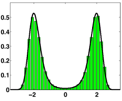
Figure 1: (a) The target density $p_{o}(x)$ (solid line) and the normalized histogram of the samples generated using the proposed scheme and with $N=10$. (b) The mean acceptance probability of jumping in a new state, depending on the number of tries $N$. We show the results of the technique in Pandolfi et al. (2010) (dashed line for weights $\omega_{j}^{(1)}$ and dotted line with triangles for $\omega_{j}^{(3)}$) and our method (squares for $\omega_{j}^{(1)}$, solid line with $\omega_{j}^{(2)}$, and with circles with $\omega_{j}^{(3)}$). (c) Estimated linear correlation coefficient depending on the number of tries $N$ for the different techniques.

6 Discussion

In this work, we have introduced a Metropolis scheme with multiple correlated points where the weight functions are not defined specifically, i.e., the analytic form can be chosen arbitrarily. We proved that our novel scheme satisfies the detailed balance condition.

Our approach draws from two different approaches (Pandolfi et al., 2010; Qin and Liu, 2001) to form a novel efficient and flexible multi-point scheme.

The multi-point approach with correlated samples provides different advantages over the standard MTM. For instance, the multi-point procedure can iteratively improve the proposal pdfs in two different ways. Firstly, since the proposal pdfs can be distinct, as in Casarin et al. (2011), it is possible to tune the parameters of each proposal in every time step. Secondly, since the candidates are generated sequentially, successive proposal pdfs can be improved learning from the previously produced samples during the same time step.

Moreover, in our technique, the only constraints of the weight functions are that they must be bounded and positive, unlike in the existing multi-point Metropolis algorithm (Qin and Liu, 2001) which is based on a specific definition of the weight functions. Here the weights can be chosen with respect to some criteria such as improving performance or reducing computational complexity. Thus our method avoids any control or check the existence of a suitable function $\lambda$ and, therefore, the selection of the weight functions is broader and easier.

It is interesting to observe that, in general, the function $\lambda$ may depend on the proposal pdf for a specific choice of weights and, in some cases, may entail certain constraints on the proposal pdf (such as that it be symmetric, for instance). An important consequence of this, it is that the weights can be chosen independently of the specific proposal pdf used in the algorithm. Namely, the proposal distribution and the weight functions can be selected separately, to fit well to the specific problem and to improve the performance of the technique. However, further theoretical or empirical studies are needed to determine the best choice of weight functions given a certain proposal and target density.

Furthermore, unlike in Pandolfi et al. (2010), in our method the weights can depend on the previous candidates, and the dimension of the weight functions grows from $\mathbb{R}^{2}$ to $\mathbb{R}^{N}$, thus being more general and potentially more powerful. Figure 2 illustrates the relationships among different MTM schemes according to the flexibility in the choice of the proposal and weight functions. Finally, we have also shown a numerical simulation and a simple multi point scheme that provides good performances reducing the correlation in the produced chain.

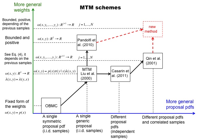
Figure 2: Comparison of different MTM schemes in literature according to the flexibility in the choice of the proposal and weight functions. With the acronym OBMC we indicate the orientational bias Monte Carlo introduced by Frenkel and Smit (1996).

7 Acknowledgements

We would like to thank the Reviewer for his comments which have helped us to improve the first version of manuscript. Moreover, this work has been partially supported by Ministerio de Ciencia e Innovación of Spain (project MONIN, ref. TEC-2006-13514-C02- 01/TCM, Program Consolider-Ingenio 2010, ref. CSD2008- 00010 COMONSENS, and Distribuited Learning Communication and Information Processing (DEIPRO) ref. TEC2009-14504-C02-01) and Comunidad Autonoma de Madrid (project PROMULTIDIS-CM, ref. S-0505/TIC/0233).

References

• Andrieu and Moulines (2006) Andrieu, C., Moulines, E., 2006. On the ergodicity properties of some adaptive MCMC algorithms. The Annals of Applied Probability 16 (3), 1462–1505.
• Casarin et al. (2011) Casarin, R., Craiu, R., Leisen, F., 2011. Interacting multiple try algorithms with different proposal distributions. To appear in Statistics and Computing, DOI: 10.1007/s11222–011–9301–9.
• Frenkel and Smit (1996) Frenkel, D., Smit, B., 1996. Understanding molecular simulation: from algorithms to applications. Academic Press, San Diego.
• Hastings (1970) Hastings, W. K., 1970. Monte Carlo sampling methods using Markov chains and their applications. Biometrika 57 (1), 97–109.
• Liang et al. (2010) Liang, F., Liu, C., Caroll, R., 2010. Advanced Markov Chain Monte Carlo Methods: Learning from Past Samples. Wiley Series in Computational Statistics, England.
• Liu (2004) Liu, J. S., 2004. Monte Carlo Strategies in Scientific Computing. Springer.
• Liu et al. (2000) Liu, J. S., Liang, F., Wong, W. H., March 2000. The multiple-try method and local optimization in metropolis sampling. Journal of the American Statistical Association 95 (449), 121–134.
• Metropolis et al. (1953) Metropolis, N., Rosenbluth, A., Rosenbluth, M., Teller, A., Teller, E., 1953. Equations of state calculations by fast computing machines. Journal of Chemical Physics 21, 1087–1091.
• Pandolfi et al. (2010) Pandolfi, S., Bartolucci, F., Friel, N., 2010. A generalization of the Multiple-try Metropolis algorithm for Bayesian estimation and model selection. Journal of Machine Learning Research (Workshop and Conference Proceedings Volume 9: AISTATS 2010) 9, 581–588.
• Qin and Liu (2001) Qin, Z. S., Liu, J. S., 2001. Multi-Point Metropolis method with application to hybrid Monte Carlo. Journal of Computational Physics 172, 827–840.
• Robert and Casella (2004) Robert, C. P., Casella, G., 2004. Monte Carlo Statistical Methods. Springer.
• Storvik (2011) Storvik, G., February 2011. On the flexibility of Metropolis-Hastings acceptance probabilities in auxiliary variable proposal generation. Scandinavian Journal of Statistics 38 (2), 342–358.