Numerical Study of Blowup in the Davey-Stewartson System

Abstract.

Nonlinear dispersive partial differential equations such as the nonlinear Schrödinger equations can have solutions that blow-up. We numerically study the long time behavior and potential blowup of solutions to the focusing Davey-Stewartson II equation by analyzing perturbations of the lump and the Ozawa exact solutions. It is shown in this way that the lump is unstable to both blowup and dispersion, and that blowup in the Ozawa solution is generic.

1. Introduction

The Davey-Stewartson (DS) system models the evolution of weakly nonlinear water waves that travel predominantly in one direction for which the wave amplitude is modulated slowly in two horizontal directions [8], [9]. It is also used in plasma physics [20, 21], to describe the evolution of a plasma under the action of a magnetic field. The DS system can be written in the form

(1) $$\begin{array}[]{ccc}i\partial_{t}u+\partial_{xx}u-\alpha\partial_{yy}u+2\rho\left(\Phi+\left|u\right|^{2}\right)u&=&0,\\ \partial_{xx}\Phi+\beta\partial_{yy}\Phi+2\partial_{xx}\left|u\right|^{2}&=&0,\end{array}$$

where $\alpha$, $\beta$ and $\rho$ take the values $\pm 1$, and where $\Phi$ is a mean field. The DS equations can be seen as a two-dimensional nonlinear Schrödinger (NLS) equation with a nonlocal term if the equation for $\Phi$ can be solved for given boundary conditions. They are classified [12] according to the ellipticity or hyperbolicity of the operators in the first and second line in (1). The case $\alpha=\beta$ is completely integrable [1] and thus provides a $2+1$-dimensional generalization of the integrable NLS equation in $1+1$ dimensions with a cubic nonlinearity. The integrable cases are elliptic-hyperbolic called DS I, and the hyperbolic-elliptic called DS II. For both there is a focusing ($\rho=-1$) and a defocusing ($\rho=1$) version. The complete integrability of the DS equation implies that it has an infinite number of conserved quantities, for instance the $L_{2}$ norm and the energy

$$E[u(t)] :=\frac{1}{2}\int_{\mathbb{T}^{2}}\bigg{[}|\partial_{x}u(t,x,y)|^{2}-|\partial_{y}u(t,x,y)|^{2}$$

$$\left.-\rho\left(|u(t,x,y)|^{4}-\frac{1}{2}\left(\Phi(t,x,y)^{2}+(\partial_{x}^{-1}\partial_{y}\Phi(t,x,y))^{2}\right)\right)\right]dxdy.$$

DS reduces to the cubic NLS in one dimension if the potential is independent of $y$, and if $\Phi$ satisfies certain boundary conditions (for instance rapidly decreasing at infinity or periodic). In the following, we will only consider the case DS II ($\alpha=1$) since the mean field $\Phi$ is then obtained by inverting an elliptic operator. The non-integrable elliptic-elliptic DS is very similar to the $2+1$ dimensional NLS equation, see for instance [12] and [6] for numerical simulations, and is therefore not studied here.

There exist many explicit solutions for the integrable cases which thus allow to address the question about the long time behavior of solutions for given initial data. For the famous Korteweg-de Vries (KdV) equation, it is known that general initial data are either radiated away or asymptotically decompose into solitons. The DS II system and the two-dimensional integrable generalization of KdV known as the Kadomtsev-Petviashvili I (KP I) equation have so-called lump solutions, a two-dimensional soliton which is localized in all spatial directions with an algebraic falloff towards infinity. For KP I it was shown [2] that small initial data asymptotically decompose into radiation and lumps. It is conjectured that this is also true for general initial data.

For the defocusing DS II global existence in time was shown by Fokas and Sung [10] for solutions of certain classes of Cauchy problems. These initial data will simply disperse. The situation is more involved for the focusing case. Pelinovski and Sulem [24] showed that the lump solution is spectrally unstable. In addition the focusing NLS equations in $2+1$ dimensions with cubic nonlinearity have the critical dimension, i.e., solutions from smooth initial data can have blowup. This means that the solutions lose after finite time the regularity of the initial data, a norm of the solution or of one of its derivatives becomes infinite. For focusing NLS equations in $2+1$ dimensions, it is known that blowup is possible if the energy of the initial data is greater than the energy of the ground state solution, see e.g. [27] and references therein, and [19] for an asymptotic description of the blowup profile. For the focusing DS II equation Sung [28] gave a smallness condition on the Fourier transform $\mathcal{F}[u_{0}]$ of the initial data to establish global existence in time for solutions to Cauchy problems

(2) $$||\mathcal{F}[u_{0}]||_{L_{1}}||\mathcal{F}[u_{0}]||_{L_{\infty}}<\frac{\pi^{3}}{2}\left(\frac{\sqrt{5}-1}{2}\right)^{2}\sim 5.92\ldots.$$

with initial data $u_{0}\in L_{p}$, $1\leq p<2$ with a Fourier transform $\mathcal{F}[u_{0}]\in L_{1}\cap L_{\infty}$.

It is not known whether there is generic blowup for initial data not satisfying this condition, nor whether the condition is optimal. Since the initial data studied in this paper are not in this class, we cannot provide further insight into this question. An explicit solution with blowup for lump-like initial data was given by Ozawa [22]. It has an $L_{\infty}$ blowup in one point ($x_{c},y_{c},t_{c}$) and is analytic for all other values of $(x,y,t)$. It is unknown whether this is the typical blowup behavior for the focusing DS II equation.

From the point of view of applications, a blowup of a solution does not mean that the studied equation is not relevant in this context. It just indicates the limit of the used approximation. It is thus of particular interest, not only in mathematics, but also in physics, since it shows the limits of the applicability of the studied model. This breakdown of the model will also in general indicate how to amend the used approximations.

In view of the open analytical questions concerning blowup in DS II solutions, we study the issue in the present paper numerically, which is a highly non-trivial problem for several reasons: first DS is a purely dispersive equation which means that the introduction of numerical dissipation has to be avoided as much as possible to preserve dispersive effects such as rapid oscillations. This makes the use of spectral methods attractive since they are known for minimal numerical dissipation and for their excellent approximation properties for smooth functions. But the algebraic falloff of both the lump and the Ozawa solution leads to strong Gibbs phenomena at the boundaries of the computational domain if the solutions are periodically continued there. We will nonetheless use Fourier spectral methods because they also allow for efficient time integration algorithms which should be ideally of high order to avoid a pollution of the Fourier coefficients due to numerical errors in the time integration.

An additional problem is the modulational instability of the focusing DS II equation, i.e., a self-induced amplitude modulation of a continuous wave propagating in a nonlinear medium, with subsequent generation of localized structures, see for instance [3, 7, 11] for the NLS equation. Thus to address numerically questions of stability and blowup of its solutions, high resolution is needed which cannot be achieved on single processor computers. Therefore we use parallel computers to study the related questions. The use of Fourier spectral method is also very convenient in this context, since for a parallel spectral code only existing optimized serial FFT algorithms are necessary. In addition such codes are not memory intensive, in contrast to other approaches such as finite difference or finite element methods. The first numerical studies of DS were done by White and Weideman [32] using Fourier spectral methods for the spatial coordinates and a second order time splitting scheme. Besse, Mauser and Stimming [6] used essentially a parallel version of this code to study the Ozawa solution and blowup in the focusing elliptic-elliptic DS equation. McConnell, Fokas and Pelloni [18] used Weideman’s code to study numerically DS I and DS II, but did not have enough resolution to get conclusive results for the blowup in perturbations of the lump in the focusing DS II case. In this paper we repeat some of their computations with considerably higher resolution.

We use a parallelized version of a fourth order time splitting scheme which was studied for DS in [17]. Obviously it is non-trivial to decide numerically whether a solution blows up or whether it just has a strong maximum. To allow to make nonetheless reliable statements, we perform a series of tests for the numerics. First we test the code on known exact solutions with algebraic falloff, the lump and the Ozawa solution. We establish that energy conservation can be used to judge the quality of the numerics if a sufficient spatial resolution is givem. It is shown that the splitting code continues to run in general beyond a potential blowup which makes it difficult to decide whether there is blowup. We argue at examples for the quintic NLS in $1+1$ dimensions (which is known to have blowup solutions) and the Ozawa solution that energy conservation is a reliable indicator in this case since the energy of the solution changes completely after a blowup, whereas it will be in accordance with the numerical accuracy after a strong maximum. Thus we reproduce well known blowup cases in this way and establish with the energy conservation a criterion to ensure the accuracy of the numerics also in unknown cases. Then we study perturbations of the lump and the Ozawa solution to see when blowup is actually observed.

The paper is organized as follows: in section 2, we describe the numerical code and its parallelization, and study as an example the lump solution. In section 3 we numerically study blowup in the focusing 1+1-dimensional quintic NLS and the Ozawa solution for DS II. In section 4 we discuss perturbations of the lump, and in section 5 perturbations of the Ozawa solution. In section 6 we give some concluding remarks.

2. Numerical methods

In this paper we are interested in the numerical study of solutions to the focusing DS II equation for initial data with algebraic falloff towards infinity in all spatial directions. This algebraic decrease of the initial data and consequently of the solution for all times is in principle not an ideal setting for the use of Fourier methods since the periodic continuation of the function at the boundaries of the computational domain will lead to Gibbs phenomena.

Nonetheless there are several reasons for the use of Fourier methods in this case: First the DS equation is a purely dispersive PDE, and we are interested in dispersive effects. Thus it important to use numerical methods that introduce as little numerical dissipation as possible, and spectral methods are especially effective in this context. Furthermore the discrete Fourier transform can be efficiently computed with a fast Fourier transform (FFT). In addition Fourier methods allow to use splitting techniques for the time integration as explained below in a very efficient way. Last but not least the focusing DS II equation is known to have a modulation instability which makes the use of high resolution necessary, especially close to the blowup situations we want to study. This instability leads to an artificial increase of the high wave numbers which eventually breaks the code, if not enough spatial resolution is provided (see for instance [16] for the focusing NLS equation). It is not possible to reach the necessary resolution on single processors which makes a parallelization of the code obligatory. As explained below, this can be conveniently done for 2-dimensional (even for 3-dimensional) Fourier transformations where the task of the 1-dimensional FFTs is performed simultaneously by several processors. This reduces also the memory requirements per processor over alternative approaches.

2.1. Splitting Methods

Splitting methods are very efficient if an equation can be split into two or more equations which can be directly integrated. They are unconditionally stable. The motivation for these methods is the Trotter-Kato formula [31, 15]

(3) $${\lim}_{n\rightarrow\infty}\left(e^{-tA/n}e^{-tB/n}\right)^{n}=e^{-t\left(A+B\right)}$$

where $A$ and $B$ are certain unbounded linear operators, for details see [15]. In particular this includes the cases studied by Bagrinovskii and Godunov in [5] and by Strang [26]. For hyperbolic equations, first references are Tappert [30] and Hardin and Tappert [14] who introduced the split step method for the NLS equation.

The idea of these methods for an equation of the form $u_{t}=\left(A+B\right)u$ is to write the solution in the form

$$u(t)=\exp(c_{1}tA)\exp(d_{1}tB)\exp(c_{2}tA)\exp(d_{2}tB)\cdots\exp(c_{k}tA)\exp(d_{k}tB)u(0)$$

where $(c_{1},\,\ldots,\,c_{k})$ and $(d_{1},\,\ldots,\,d_{k})$ are sets of real numbers that represent fractional time steps. Yoshida [33] gave an approach which produces split step methods of any even order. The DS equation can be split into

(4) $$i\partial_{t}u=(-\partial_{xx}u+\alpha\partial_{yy}u),\,\,\,\partial_{xx}\Phi+\alpha\partial_{yy}\Phi+2\partial_{xx}\left(\left|u\right|^{2}\right)=0,$$

(5) $$i\partial_{t}u=-2\rho\left(\Phi+\left|u\right|^{2}\right)u,$$

which are explicitly integrable, the first two in Fourier space, equation (5) in physical space since $|u|^{2}$ and thus $\Phi$ is constant in time for this equation. Convergence of second order splitting along these lines was studied in [6]. We use here fourth order splitting as given in [33] and already studied in [17] for the DS II equation. In the latter reference, it was shown that this scheme is very efficient in this context. The method is convenient for parallel computing, because of easy coding (loops) and low memory requirements.

Notice that the splitting method in the form (5) conserves the $L_{2}$ norm: the first equation implies that its solution in Fourier space is just the initial condition (from the last time step) multiplied by a factor $e^{i\phi}$ with $\phi\in\mathbb{R}$. Thus the $L_{2}$ norm is constant for solutions to this equation because of Parseval’s theorem. The second equation as mentioned conserves the $L_{2}$ norm exactly. Thus the used splitting scheme has the conservation of the $L_{2}$ norm implemented. As we will show in the following, this does not guarantee the accuracy of the numerical solution since other conserved quantities as the energy the conservation of which is not implemented might not be numerically conserved. In fact we will show that the numerically computed energy provides a valid indicator of the quality of the numerics.

2.2. Parallelization of the code

Since high resolution is needed to numerically examine the focusing DS II equation, the code is parallelized to reduce the wall clock time required to run the simulation and to allow the problem to fit in memory. The runs typically used $N_{x}=N_{y}=2^{15}$, where $N_{x}$ and $N_{y}$ denote the number of Fourier modes in $x$ and $y$ respectively. The parallelization is done by a slab domain decomposition. The grid points are given by

$$x_{n}=\frac{2\pi nL_{x}}{N_{x}},\quad y_{m}=\frac{2\pi mL_{y}}{N_{y}},$$

so that the numerical solution is in the computational domain

$$x\times y\in[-L_{x}\pi,L_{x}\pi]\times[-L_{y}\pi,L_{y}\pi].$$

In the computations, $L_{x}=L_{y}$ is chosen large enough so that the numerical solution is small at the boundaries, and hence a numerical solution on a periodic domain can be considered as a good approximation to the solution on an unbounded domain. The approximate solution $u$ is represented by an $N_{x}\times N_{y}$ matrix, which is distributed among the MPI processes (note that each MPI process uses a single core). For programming ease and for the efficiency of the Fourier transform, $N_{x}$ and $N_{y}$ are chosen to be powers of two. The number of MPI processes, $n_{p}$ is chosen to divide $N_{x}$ and $N_{y}$ perfectly, so that each process holds $N_{x}\times N_{y}/n_{p}$ elements of $u$, for example process $i$ holds the elements

$$u(1:N_{x},(i-1)\frac{N_{y}}{n_{p}}+1:i\frac{N_{y}}{n_{p}})$$

in the global array. To avoid performing global Fourier transforms which are inefficient, the array is transposed once all the one dimensional Fourier transforms in the $x$ direction have been done. Since the data is evenly distributed among the MPI processes, this transpose is efficiently implemented using MPI_ALLTOALL [13]. After the transpose, the Fourier transform $\hat{u}$ is distributed on the processes so that process $i$ holds the elements corresponding to

$$\hat{u}((i-1)\frac{N_{x}}{n_{p}}+1:\frac{iN_{x}}{n_{p}},1:Ny),$$

on which the second set of one dimensional FFTs can be done. The one dimensional FFTs were done using FFTW 3.0, FFTW 3.1 and FFTW 3.2 which are close to optimal on x86 architectures and allow the resulting program to be portable but still simple.

2.3. Lump solution of the focusing DS II equation

To test the performance of the code, we first propagate initial data from known exact solutions and compare the numerical and the exact solution at a later time.

The focusing DS II equation has solitonic solutions which are regular for all $x,y,t$, and which are localized with an algebraic falloff towards infinity, known as lumps [4]. The single lump is given by

(6) $$u(x,y,t)=2c\frac{\exp\left(-2i(\xi x-\eta y+2(\xi^{2}-\eta^{2})t)\right)}{|x+4\xi t+i(y+4\eta t)+z_{0}|^{2}+|c|^{2}}$$

where $(c,z_{0})\in\mathbb{C}^{2}$ and $(\xi,\eta)\in\mathbb{R}^{2}$ are constants. The lump moves with constant velocity $(-2\xi,-2\eta)$ and decays as $(x^{2}+y^{2})^{-1}$ for $x,y\to\infty$.

We choose $N_{x}=N_{y}=2^{14}$ and $L_{x}=L_{y}=50$, with $\xi=0,\eta=-1,z_{0}=1$ and $c=1$. The large values for $L_{x}$ and $L_{y}$ are necessary to ensure that the solution is small at the boundaries of the computational domain to reduce Gibbs phenomena. The difference for the mass of the lump and the computed mass on this periodic setting is of the order of $6*10^{-5}$. The initial data for $t=-6$ are propagated with $N_{t}=1000$ time steps until $t=6$. In Fig. 1 contours of the solution at different times are shown. Here and in the following we always show closeups of the solution. The actual computation is done on the stated much larger domain. In this paper we will always show the square of the modulus of the complex solution for ease of presentation. The time dependence of the $L_{2}$ norm of the difference between the numerical and the exact solution can be also seen there.

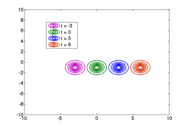
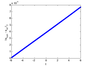
Figure 1. Contours of $|u|^{2}$ on the left and a plot of $||u_{exact}-u_{num}||_{2}$ on the right in dependence of time for the solution to the focusing DS II equation (1) for lump initial data (6).

The numerical error is here mainly due to the lack of resolution in time. Since the increase in the number of time steps is computationally expensive, a fourth order scheme is very useful in this context. The spatial resolution can be seen from the modulus of the Fourier coefficients at the final time of computation $t=6$ in Fig. 2. It decreases to $10^{-6}$, thus essentially the value for the initial data. For computational speed considerations we always use double precision which because of finite precision arithmetic give us a range of 15 orders of magnitude. Since function values computed using the split step method were for most of the computation of order 1, and less than 5,000, rounding errors allow for a precision of $10^{-14}$ when less than $2^{15}\times 2^{15}$ Fourier modes are used. When more modes than $2^{15}\times 2^{15}$ were used, we found a reduction in precision. Despite the algebraic falloff of the solution we have a satisfactory spatial resolution because of the large computational domain and the high resolution. The modulational instability does not show up in this and later examples before blowup.

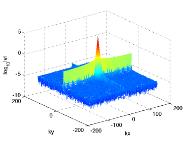
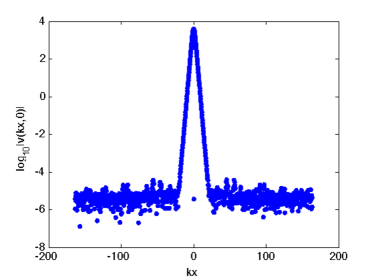
Figure 2. Fourier coefficients for the situation in Fig. 1 at $t=6$.

3. Blowup for the quintic NLS in $1+1$ dimensions and the focusing DS II

It is known that focusing NLS equations can have solutions with blowup, if the nonlinearity exceeds a critical value depending on the spatial dimension. For the $1+1$ dimensional case, the critical nonlinearity is quintic, for the $2+1$ dimensional it is cubic, see for instance [27] and references therein. Thus the focusing DS II equation can have solutions with blowup. In this section we will first study numerically blowup for the $1+1$ dimensional quintic NLS equation, and then numerically evolve initial data for a known exact blowup solution to the focusing DS II equation due to Ozawa [22]. We discuss some peculiarities of the fourth order splitting scheme in this context.

3.1. Blowup for the quintic one-dimensional NLS

The focusing quintic NLS in $1+1$ dimensions has the form

(7) $$i\partial_{t}u+\partial_{xx}u+|u|^{4}u=0,$$

where $u\in\mathbb{C}$ depends on $x$ and $t$ (we consider again solutions periodic in $x$). This equation is not completely integrable, but assuming the solution is in $L_{2}$, has conserved $L_{2}$ norm and, provided the solution $u\in H_{2}$, a conserved energy,

(8) $$E[u]=\int_{\mathbb{R}}\left(\frac{1}{2}|\partial_{x}u|^{2}-\frac{1}{6}|u|^{6}\right)dx.$$

It is known that initial data with negative energy blow up for this equation in finite time, and that the behavior close to blowup is given in terms of a solution to an ODE, see [19].

As discussed in sect. 2.1, the splitting scheme we are using here has the property that the $L_{2}$ norm is conserved. Thus the quality of the numerical conservation of the $L_{2}$ norm gives no indication on the accuracy of the numerical solution. However as discussed in [16], conservation of the numerically computed energy gives a valid criterion for the quality of the numerics: in general it overestimates the $L_{\infty}$ numerical error by two orders of magnitude at the typically aimed at precisions.

If we consider as in [25] for the quintic NLS the initial data $u_{0}(x)=1.8i\exp(-x^{2})$, the energy is negative. We compute the solution with $L_{x}=5$ and $N_{x}=2^{15}$ with $N_{t}=10^{4}$ time steps. The result can be seen in Fig. 3 (to obtain more structure in the solution after the blow up due to a less pronounced maximum, the plot on the left was generated with the lower spatial resolution $N=2^{12}$).

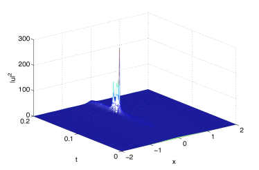
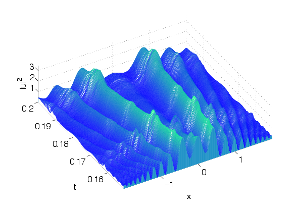
Figure 3. Solution to the focusing quintic NLS (7) for the initial data $u_{0}=1.8i\exp(-x^{2})$ with $N=2^{12}$ on the left and $N=2^{15}$ on the right for $t>t_{c}$.

The initial data clearly get focused to a strong maximum, but the code does not break. We note that this is in contrast to other fourth order schemes tested for $1+1$ dimensional NLS equations in [16], which typically produce an overflow close to the blowup. But clearly the solution shows spurious oscillations after the time $t_{c}\sim 0.155$. In fact the numerically computed energy, which will always be time-dependent due to unavoidable numerical errors, will be completely changed after this time. We consider

(9) $$\Delta_{E}=\left|1-\frac{E(t)}{E(0)}\right|,$$

where $E(t)$ is the numerically computed energy (8) and get for the example in Fig. 3 the behavior shown in Fig. 4. At the presumed blowup at $t_{c}\sim 0.155$ as in [25], the energy jumps to a completely different value. Thus this jump can and will be used to indicate blowup. To illustrate the effects of a lower resolution in time and space imposed by hardware limitations for the DS computations, we show this quantity for several resolutions in Fig. 4. If a lower resolution in time is used as in some of the DS examples in this paper, the jump is slightly smoothed out. But the plateau is still reached at essentially the same time which indicates blowup. Thus a lack of resolution in time in the given limits will not be an obstacle to identify a possible singularity. The reason for this is the use of a fourth order scheme that allows to take larger time steps. We will present computations with different resolutions to illustrate the steepening of the energy jump as above if this is within the limitations imposed by the hardware.

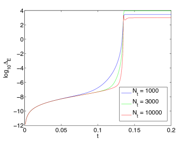
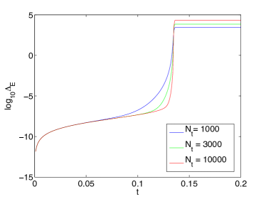
Figure 4. Numerically computed energy for the situation studied in Fig. 3 for $N=2^{12}$ on the left and $N=2^{15}$ on the right for several values of $N_{t}$. At the blowup, the energy jumps.

We show the modulus of the Fourier coefficients for $N=2^{12}$ and $N=2^{15}$ before and after the critical time in Fig. 5. It can be seen that the solution is well resolved before blowup in the latter case, and that the singularity leads to oscillations in the Fourier coefficients. A lack of spatial resolution as for $N=2^{12}$ in Fig. 5 triggers the modulation instability close to the blowup and at later times as can be seen from the modulus of the Fourier coefficients that increase for larger wavenumbers. Therefore we always aim at a sufficient resolution in space even for times close to a blowup. After this time the modulation instability will be present in the spurious solution produced by the splitting scheme as we will show for an example.

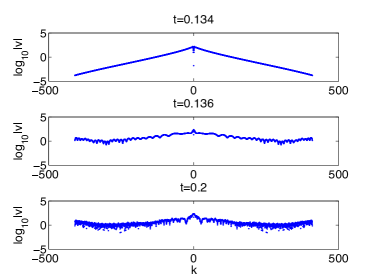
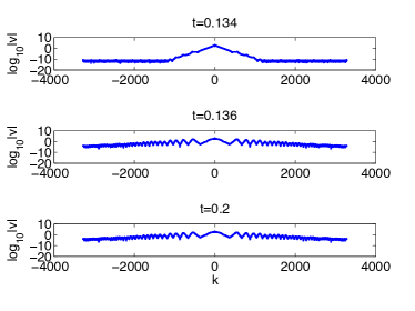
Figure 5. Fourier coefficients for the solution in Fig. 3 close to the critical and at a later time for $N=2^{12}$ on the left and $N=2^{15}$ on the right for $N_{t}=10^{4}$.

Remark 3.1.

Stinis [25] has recently computed singular solutions to the focusing quintic nonlinear Schrödinger equation in $1+1$ dimensions. This equation has solutions in $L_{\infty}L_{2}$ that may not be unique for given smooth initial data and that may exhibit blowup of the $L_{\infty}H_{1}$ norm. Following Tao [29], Stinis [25] has used a selection criteria to pick a solution after the blow up time of the $L_{\infty}H_{1}$ norm. They suggest that ‘mass’ is ejected (which means that the $L_{2}$ norm is changed) at times where the $L_{\infty}H_{1}$ norm blows up. The splitting scheme studied here in contrast produces a weak solution with a different energy since the $L_{2}$ norm conservation is built in.

3.2. Blowup in the Ozawa solution

For the focusing DS II equation, an exact solution was given by Ozawa [22] which is in $L_{2}$ for all times with an $L_{\infty}$ blowup in finite time. We can summarize his results as follows:

Theorem 3.1 (Ozawa).

Let $ab<0$ and $T=-a/b$. Denote by $u(x,y,t)$ the function defined by

(10) $$u(x,y,t)=\exp\left(i\frac{b}{4(a+bt)}(x^{2}-y^{2})\right)\frac{v(X,Y)}{a+bt}$$

where

(11) $$v(X,Y)=\frac{2}{1+X^{2}+Y^{2}},\,\,X=\frac{x}{a+bt},\,\,Y=\frac{y}{a+bt}$$

Then, $u$ is a solution of (1) with

(12) $$\|u(x,y,t)\|_{2}=\|v(X,Y)\|_{2}=2\sqrt{\pi}$$

and

(13) $$|u(t)|^{2}\rightarrow 2\pi\delta\,\,\mbox{when}\,\,t\rightarrow T.$$

where $\delta$ is the Dirac measure.

We thus consider initial data of the form

(14) $$u(x,y,0)=2\frac{\exp\left(-i(x^{2}-y^{2})\right)}{1+x^{2}+y^{2}}$$

($a=1$ and $b=-4$ in (10)). As for the quintic NLS in $1+1$ dimensions, we always trace the conserved energy for DS II (1).

The computation is carried out with $N_{x}=N_{y}=2^{15}$, $L_{x}=L_{y}=20$, and $N_{t}=1000$ respectively $N_{t}=4000$; we show the solution at different times in Fig. 6. The difference of the Ozawa mass and the computed $L_{2}$ norm on the periodic setting is of the order of $9*10^{-5}$.

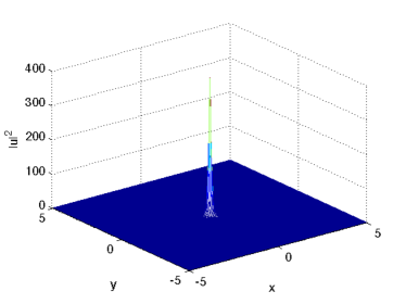
Figure 6. Solution to the focusing DS II equation (1) for $t=0.075$ and $t=0.15$ in the first row and $t=0.225$ and $t=0.3$ below for an initial condition of the form (14).

The time evolution of $\underset{x,y}{\max}|u(x,y,t)|^{2}$ and the difference between the numerical and the exact solution can be seen in Fig. 7 (the critical time $t_{c}$ is not on the shown grid, thus the solution is always finite on the grid points). The code continues to run after the critical time, but the numerical solution obviously no longer represents the Ozawa solution.

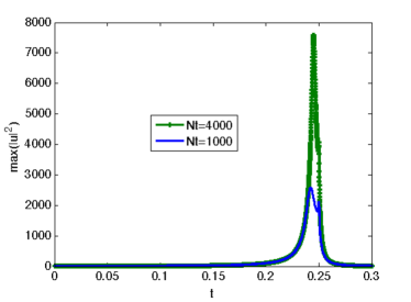
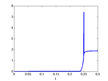
Figure 7. Time evolution of $max(|u_{num}|^{2})$ and of $\|u_{num}-u_{exact}\|_{2}$ for the situation in Fig. 6.

The numerically computed energy jumps at the blow up time as can be seen in Fig. 8.

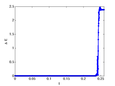
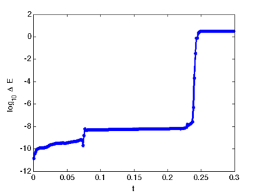
Figure 8. Numerically computed energy $E(t)$ and $\Delta E=|1-E(t)/E(0)|$ (9) for the situation in Fig. 6.

The Fourier coefficients at $t=0.15$ are shown in Fig. 9. Despite the Gibbs phenomenon the Fourier coefficients for the initial data decrease to $10^{-8}$. Spatial resolution is still satisfactory at half the blowup time.

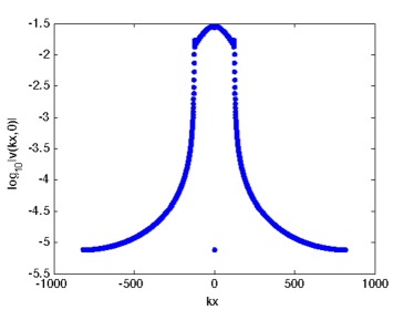
Figure 9. Fourier coefficients of $u$ at $t=0.15$ for an initial condition of the form (14).

Remark 3.2.

The jump of the computed energy at blowup is dependent on sufficient spatial resolution as can be seen in Fig. 10 for the example of the quintic NLS of Fig. 4 and the Ozawa solution in Fig. 8. For low resolution blow-up can be still clearly recognized from the computed energy, but the energy does not stay on the level at blow-up.

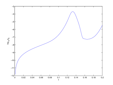
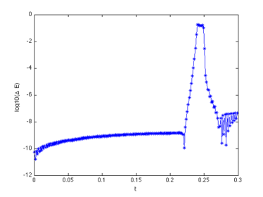
Figure 10. Computed numerical energy for quintic NLS in Fig. 4 with $N=2^{8}$ and for the Ozawa solution in Fig. 8 with $N_{x}=N_{y}=2^{12}$.

4. Perturbations of the lump solution

In this section we consider perturbations of the lump solution (6). First we propagate initial data obtained from the lump after multiplication with some scalar factor. Then we consider a perturbation with a Gaussian and a deformed lump.

4.1. Perturbation of the lump by rescaled initial data

We first consider rescaled initial data from the lump (6) denoted by $u_{l}$

$$u(x,y,-6)=Au_{l},$$

where $A\in\mathbb{R}$ is a scaling factor. The computations are carried out with $N_{x}=N_{y}=2^{14}$ points for $x\times y\in[-50\pi,50\pi]\times[-50\pi,50\pi]$ and $t\in[-6,6]$.

For $A=1.1$, and $N_{t}=1000$, we observe a blowup of the solution at $t_{c}\sim 1.6$. The time evolution of $\underset{x,y}{\max}|u(x,y,t)|^{2}$ and of the energy is shown in Fig. 11. The maximum of $|u|^{2}$ in Fig. 11 is clearly smaller than in the case of the Ozawa solution. This is due to the lower resolution in time which is used for this computation. Nevertheless, the jump in the energy is obviously present.

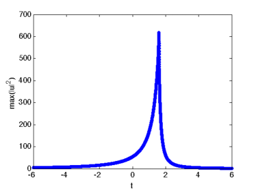
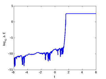
Figure 11. Evolution of $max(|u|^{2})$ and the numerically computed energy in dependence of time for a solution to the focusing DS II equation (1) for an initial condition of the form $u(x,y,-6)=1.1u_{l}$.

The Fourier coefficients at $t=0$ can be seen in Fig. 12. They again decrease by almost 6 orders of magnitude.

To illustrate the modulational instability at a concrete example, we show the Fourier coefficients after the critical time in Fig. 13. It can be seen that the modulus of the coefficients of the high wavenumbers increases instead of decreasing as to be expected for smooth functions. This indicates once more that the computed solution after the blowup time has to be taken with a grain of salt.

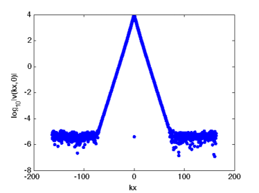
Figure 12. Fourier coefficients at $t=0$ for a solution to the focusing DS II equation (1) for an initial condition of the form $u(x,y,-6)=1.1u_{l}$.

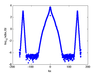
Figure 13. Fourier coefficients at $t=6$ for a solution to the focusing DS II equation (1) for an initial condition of the form $u(x,y,-6)=1.1u_{l}$.

For $A=0.9$, the initial pulse travels in the same direction as the exact solution, but loses speed and height and is broadened, see Fig. 14. It appears that this modified lump just disperses asymptotically. The solution can be seen in Fig. 15. Its Fourier coefficients in Fig. 16 show that the resolution of the initial data is almost maintained.

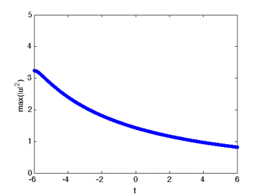
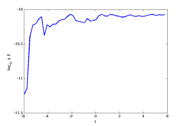
Figure 14. Evolution of $max(|u|^{2})$ and the numerically computed energy in dependence of time for a solution to the focusing DS II equation (1) for an initial condition of the form $u(x,y,-6)=0.9u_{l}$.

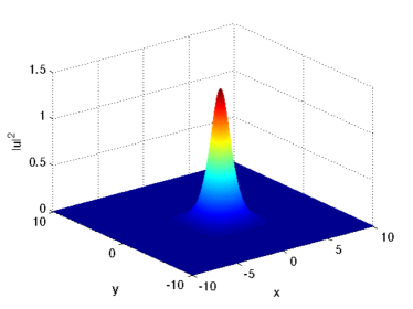
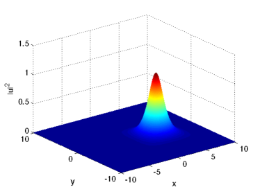
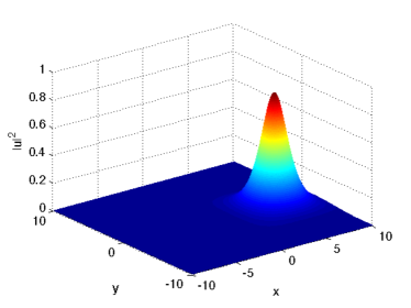
Figure 15. Solution to the focusing DS II equation (1) for an initial condition of the form $u(x,y,-6)=0.9u_{l}$ for $t=-3$ and $t=0$ in the first row and $t=3$ and $t=6$ below.

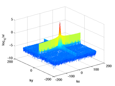
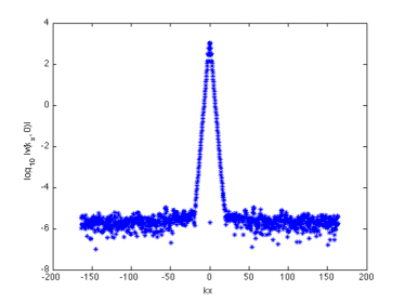
Figure 16. The Fourier coefficients at $t=0$ of the solution to the focusing DS II equation (1) for an initial condition of the form $u(x,y,-6)=0.9u_{l}$.

4.2. Perturbation of the lump with a Gaussian

We consider an initial condition of the form

(15) $$u(x,y,-6)=u_{l}+B\exp(-(x^{2}+y^{2})),\,\,B\in\mathbb{R}.$$

For $B=0.1$ and $N_{t}=1000$, we show the solution at different times in Fig. 17. The solution travels at the same speed as before, but its amplitude varies, growing and decreasing successively, see Fig. 18.

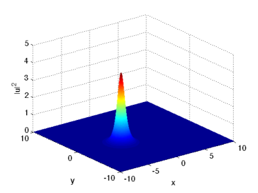
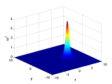
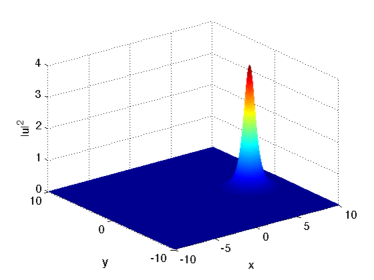
Figure 17. Solution to the focusing DS II equation (1) for an initial condition of the form (15) with $B=0.1$ for $t=-3$ and $t=0$ in the first row and $t=3$ and $t=6$ below.

The time evolution of the energy can be seen in Fig. 18. There is no indication of blowup in this example. The solution appears to disperse for $t\to\infty$.

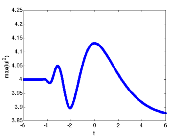
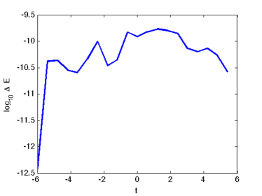
Figure 18. Evolution of $max(|u|^{2})$ and of the energy in dependence of time for an initial condition of the form (15) with $B=0.1$.

The Fourier coefficients at $t=6$ in Fig. 19 show the wanted spatial resolution.

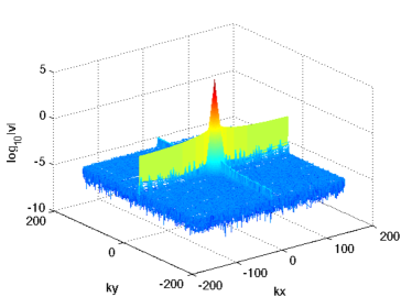
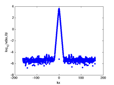
Figure 19. Fourier coefficients of $u$ at $t=6$ for an initial condition of the form (15) with $B=0.1$.

A similar behavior is observed if a larger value for the amplitude of the perturbation is chosen, e.g., $B=0.5$.

4.3. Deformation of the Lump

We consider initial data of the form

(16) $$u(x,y,-6)=u_{l}(x,\kappa y,-6),$$

i.e., a deformed (in $y$-direction) initial lump in this subsection. The computations are carried out with $N_{x}=N_{y}=2^{14}$ points for $x\times y\in[-50\pi,50\pi]\times[-50\pi,50\pi]$ and $t\in[-6,6]$.

For $\kappa=0.9$, the resulting solution loses speed and width as can be seen in Fig. 20. Its height and energy grow, but both stay finite, see Fig. 21. It is possible that the solution eventually blows up, but not on the time scales studied here.

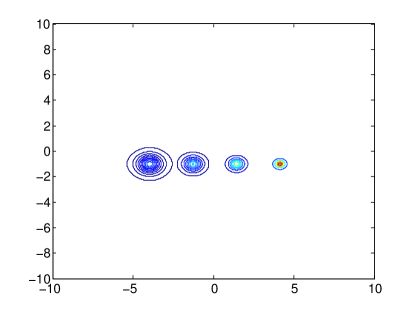
Figure 20. Contour plot for a solution to the focusing DS II equation (1) for an initial condition of the form (16) with $\kappa=0.9$ for different times.

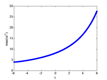
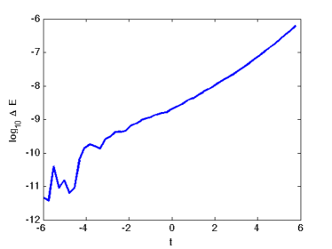
Figure 21. Evolution of $max(|u|^{2})$ and the numerically computed energy in dependence of time for the focusing DS II equation (1) for an initial condition of the form (16) with $\kappa=0.9$.

The Fourier coefficients at $t=0$ in Fig. 22 show the wanted spatial resolution.

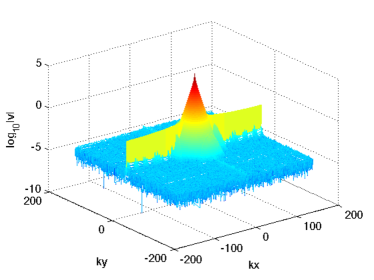
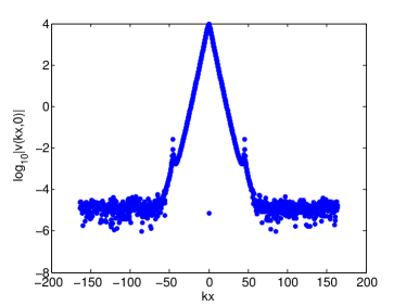
Figure 22. Fourier coefficients of the solution to the focusing DS II equation (1) for an initial condition of the form (16) with $\kappa=0.9$ at $t=0$.

For $\kappa=1.1$, we observe the opposite behavior in Fig. 23. The solution travels with higher speed than the initial lump and is broadened. The energy does not show any sudden change, see Fig. 24. It seems that the initial pulse will asymptotically disperse. The Fourier coefficients at $t=0$ in Fig. 25 show the wanted spatial resolution.

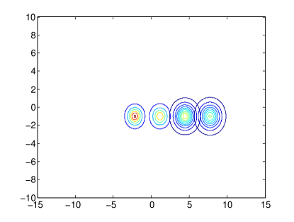
Figure 23. Contour plot for a solution to the focusing DS II equation (1) for an initial condition of the form (16) with $\kappa=1.1$ for different times.

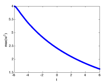
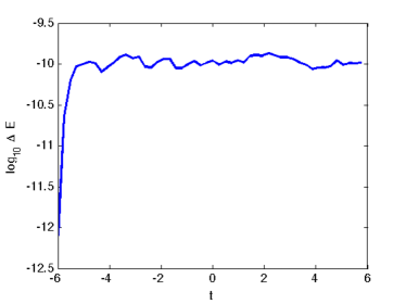
Figure 24. Evolution of $max(|u|^{2})$ and the numerically computed energy $E$for a solution to the focusing DS II equation (1) for an initial condition of the form (16) with $\kappa=1.1$.

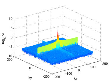
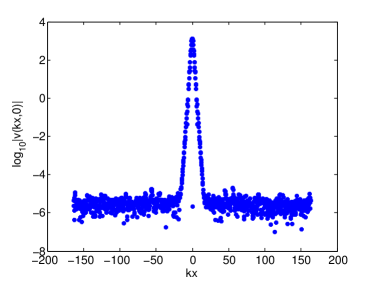
Figure 25. Fourier coefficients of the solution to the focusing DS II equation (1) for an initial condition of the form (16) with $\kappa=1.1$ at $t=0$.

5. Perturbations of the Ozawa solution

In this section we study as for the lump in the previous section various perturbations of initial data for the Ozawa solution to test whether blowup is generic for the focusing DS II equation.

5.1. Perturbation of the Ozawa solution by multiplication with a scalar factor

We consider initial data of the form

(17) $$u(x,y,0)=2C\frac{\exp\left(-i(x^{2}-y^{2})\right)}{1+x^{2}+y^{2}},$$

i.e., initial data of the Ozawa solution multiplied by a scalar factor. The computation is carried out with $N_{x}=N_{y}=2^{15}$ points for $x\times y\in[-20\pi,20\pi]\times[-20\pi,20\pi]$.

For $C=1.1$, and $N_{t}=2000$, we show the behavior of $|u|^{2}$ at different times in Fig. 26.

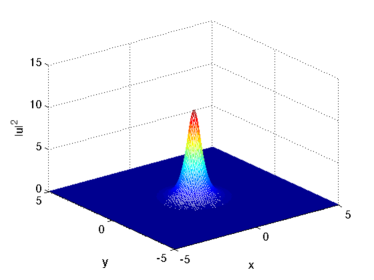
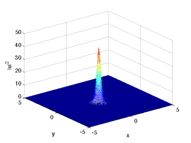
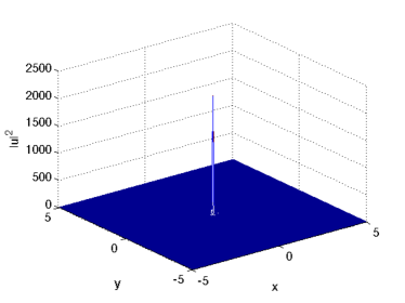
Figure 26. Solution to the focusing DS II equation (1) for an initial condition of the form (17) with $C=1.1$ for $t=0.075$ and $t=0.15$ in the first row and $t=0.225$ and $t=0.3$ below.

The time evolution of $\underset{x,y}{\max}|u(x,y,t)|^{2}$ and the numerically computed energy are shown in Fig. 27. We observe an $L_{\infty}$ blowup at the time $t_{c}\sim 0.2210$.

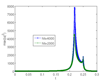
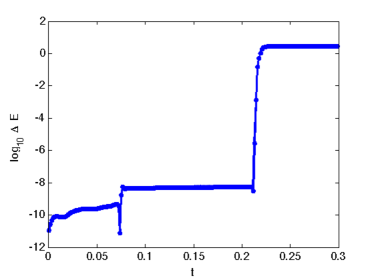
Figure 27. Evolution of $max(|u|^{2})$ and the numerically computed energy for an initial condition of the form (17) with $C=1.1$.

The Fourier coefficients at $t=0.15$ (before the blowup) in Fig. 28 show the wanted spatial resolution.

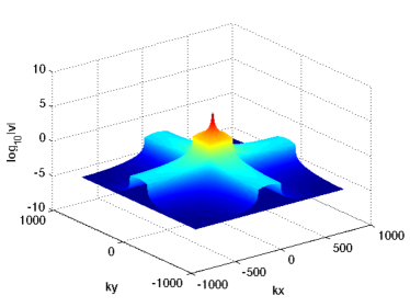
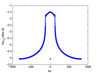
Figure 28. Fourier coefficients of solution to the focusing DS II equation (1) for an initial condition of the form (17) with $C=1.1$ at $t=0.15$.

For $C=0.9$, the initial pulse grows until it reaches its maximal height at $t=0.2501$, but there is no indication for blowup, see Fig. 29.

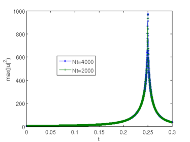
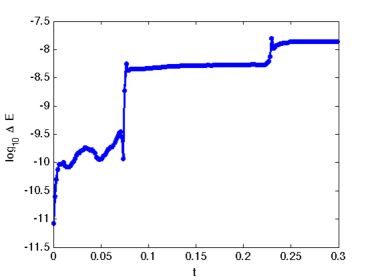
Figure 29. Evolution of $max(|u|^{2})$ in dependence of time, for an initial condition of the form (17) with $C=0.9$.

The solution at different times can be seen in Fig. 30.

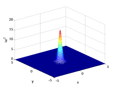
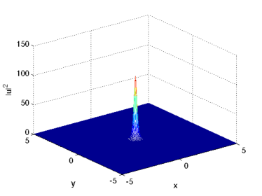
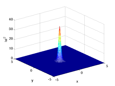
Figure 30. Solution to the focusing DS II equation (1) for an initial condition of the form (17) with $C=0.9$, $N_{t}=2000$ for $t=0.075$ and $t=0.15$ in the first row and $t=0.225$ and $t=0.3$ below.

The Fourier coefficients in Fig. 31 show again that the wanted spatial resolution is achieved.

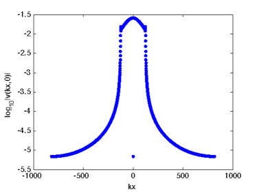
Figure 31. Fourier coefficients of the solution to the focusing DS II equation (1) at $t=0.15$ for an initial condition of the form (17) with $C=0.9$.

Thus for initial data given by the Ozawa solution multiplied with a factor $C$, we find that for $C>1$, blow up seems to occur before the critical time of the Ozawa solution, and for $C<1$ the solution grows until $t=0.25$ but does not blow up. Consequently the Ozawa initial data seem to be critical in this sense that data of this form with smaller norm do not blow up.

5.2. Perturbation of the Ozawa solution with a Gaussian

We consider an initial condition of the form

(18) $$u(x,y,0)=2\frac{\exp\left(-i(x^{2}-y^{2})\right)}{1+x^{2}+y^{2}}+D\exp(-(x^{2}+y^{2})).$$

For $D=0.1$ and $N_{t}=2000$, we show the behavior of $|u|^{2}$ at different times in Fig. 32.

Figure 32. Solution to the focusing DS II equation (1) for an initial condition of the form (18) with $D=0.1$ for $t=0.075$ and $t=0.15$ in the first row and $t=0.225$ and $t=0.3$ below .

The time evolution of $\underset{x,y}{\max}|u(x,y,t)|^{2}$ is shown in Fig. 33. We observe a jump of the energy indicating blowup at the time $t_{c}\sim 0.2332$.

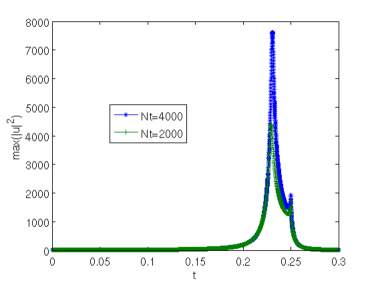
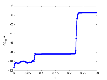
Figure 33. Evolution of $max(|u|^{2})$ and the numerically computed energy in dependence of time for the solution to the focusing DS II equation (1) for an initial condition of the form (18) with $D=0.1$.

The Fourier coefficients at $t_{c}=0.15$ in Fig. 34 show that the wanted spatial resolution is achieved.

Figure 34. Fourier coefficients of the solution to the focusing DS II equation (1) at $t=0.15$ for an initial condition of the form (18) with $D=0.1$.

The same experiment with $D=0.5$ appears again to show blow up, but at an earlier time $t_{c}\sim 0.1659$, see Fig. 35.

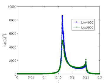
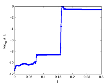
Figure 35. Evolution of $max(|u|^{2})$ and the numerically computed energy for the solution to the focusing DS II equation (1) for an initial condition of the form (18) with $D=0.5$.

Thus the energy added by the perturbation of the form $D\exp(-(x^{2}+y^{2}))$ seems to lead to a blowup before the critical time of the Ozawa solution. This means that the blowup in the Ozawa solution is clearly a generic feature at least for initial data close to Ozawa for the focusing DS II equation.

5.3. Deformation of the Ozawa solution

We study deformations of Ozawa initial data of the form

(19) $$u(x,y,0)=2\frac{\exp\left(-i(x^{2}-(\nu y)^{2})\right)}{1+x^{2}+(\nu y)^{2}},$$

i.e., a deformation in the $y$-direction. The computations are carried out with $N_{x}=N_{y}=2^{15}$ points for $x\times y\in[-20\pi,20\pi]\times[-20\pi,20\pi]$ and $t\in[0,0.3]$.

For $\nu=0.9$, we observe a maximum of the solution at $t=0.2441$, see Fig. 36, followed by a second maximum, but there is no indication of a blowup. Energy conservation is in principle high enough to indicate that the solution stays regular on the considered time scales.

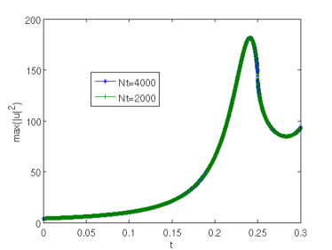
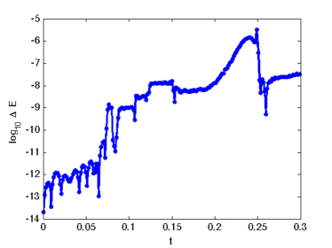
Figure 36. Evolution of $max(|u|^{2})$ and the numerically computed energy $E$ in dependence of time for a solution to the focusing DS II equation (1) for an initial condition of the form (19) with $\nu=0.9$.

The Fourier coefficients at $t=0.15$ in Fig. 37 show the wanted spatial resolution.

Figure 37. Fourier coefficients of the solution to the focusing DS II equation (1) for an initial condition of the form (19) with $\nu=0.9$ at $t=0$.

The situation is similar for $\nu=1.1$. The maximum of the solution is observed at $t=0.2254$, see Fig. 38, followed again by a second maximum. Energy conservation appears once more to rule out a blowup in this case.

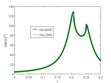
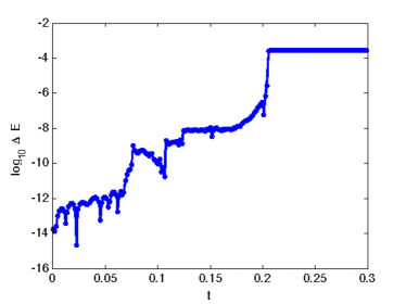
Figure 38. Evolution of $max(|u|^{2})$ and the numerically computed energy $E$ for a solution to the focusing DS II equation (1) for an initial condition of the form (19) with $\nu=1.1$.

The Fourier coefficients at $t=0.15$ in Fig. 39 again show the wanted spatial resolution.

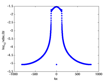
Figure 39. Fourier coefficients of the solution to the focusing DS II equation (1) for an initial condition of the form (19) with $\nu=1.1$ at $t=0.15$.

6. Conclusion

In this paper we have numerically studied long time behavior and stability of exact solutions to the focusing DS II equation with an algebraic falloff towards infinity. We have shown that the necessary resolution can be achieved with a parallelized version of a spectral code. The spatial resolution as seen at the Fourier coefficients was always well beyond typical plotting accuracies of the order of $10^{-3}$. For the time integration we used an unconditionally stable fourth order splitting scheme. As argued in [16, 17], the numerically computed energy of the solution gives a valid indicator of the accuracy for sufficient spatial resolution. To ensure the latter, we always presented the Fourier coefficients of the solution at a time before a singularity appeared. In addition we show here that the numerically computed energy indicates blowup by jumping to a different value in cases where the code runs beyond a singularity in time.

After testing the code for exact solutions, the lump and the blowup solution by Ozawa, we showed that both solutions are critical in the following sense: adding energy to it leads to a blowup for the lump, and an earlier blowup time for the Ozawa solution. For initial data with less energy, no blowup was observed in both cases, the initial data asymptotically just seem to be dispersed. This is in accordance with the conjecture in [18] that solutions to the focusing DS II equations either blow up or disperse. In particular the lump is unstable against both blowup and dispersion, in contrast to the lump of the KP I equation that appears to be stable, see for instance [23]. Note that the perturbations we considered here test the nonlinear regime of the PDE for which so far no analytical results appear to be established.

References

- [1] M. Ablowitz and R. Haberman, Nonlinear Evolution Equations in Two and Three Dimensions, Phys. Rev. Lett., 35 (1975), pp. 1185–8.
- [2] M. J. Ablowitz and A. Fokas, On the inverse scattering and direct linearizing transforms for the Kadomtsev-Petviashvili equation, Physics Letters A, 94 (1983), pp. 67–70.
- [3] G. Agrawal, Nonlinear Fiber Optics, Academic Press, San Diego, 2006.
- [4] V. Arkadiev, A. Pogrebkov, and M. Polivanov, Inverse Scattering Transform Method and Soliton Solutions for Davey-Stewartson II Equation, Physica D: Nonlinear Phenomena, 36 (1989), pp. 189–197.
- [5] K. A. Bagrinovskii and S. Godunov, Difference Schemes for multi-dimensional Problems, Dokl.Acad. Nauk., 115 (1957), pp. 431–433.
- [6] C. Besse, N. Mauser, and H. Stimming, Numerical Study of the Davey-Stewartson System, Math. Model. Numer. Anal., 38 (2004), pp. 1035–1054.
- [7] M. Cross and P. Hohenberg, Pattern formation outside of equilibrium, Rev. Mod. Phys., 65 (1993), p. 851 1112.
- [8] A. Davey and K. Stewartson, On Three-dimensional Packets of Surface Waves, Proc. R. Soc. Lond. A., 338 (1974), pp. 101–110.
- [9] V. Djordjevic and L. Redekopp, On Two-dimensional Packets of Capillarity-Gravity Waves, J. Fluid Mech., 79 part 4 (1977), pp. 703–714.
- [10] A. Fokas and L. Sung, The Inverse spectral Method for the KP I Equation without the Zero Mass Constraint, Math. Proc. Camb. Phil. Soc., 125 (1999), pp. 113–138.
- [11] M. Forest and J. Lee, Geometry and modulation theory for the periodic nonlinear Schrödinger equation, in Oscillation Theory, Computation, and Methods of Compensated Compactness, Minneapolis, MN, 1985. The IMA Volumes in Mathematics and Its Applications, vol. 2, Springer, New York, 1986, pp. 35 –69.
- [12] J.-M. Ghidaglia and J.-C. Saut, On the initial Value Problem for the Davey-Stewartson Systems, Nonlinearity, 3 (1990).
- [13] W. Gropp, E. Lusk, and A. Skjellum, Using MPI, MIT Press, Boston, 1999.
- [14] R. H. Hardin and F. D. Tappert, Applications of the Split-Step Fourier Method to the numerical Solution of nonlinear and variable Coefficient Wave Equations, SIAM Rev., 15 (1973), p. 423.
- [15] T. Kato, Trotter’s product formula for an arbitrary pair of self-adjoint contraction semigroups, vol. 3, Academic Press, Boston, 1978, pp. 185 –195.
- [16] C. Klein, Fourth-Order Time-Stepping for low Dispersion Korteweg-de Vries and nonlinear Schrödinger Equation, Electronic Transactions on Numerical Analysis., 39 (2008), pp. 116–135.
- [17] C. Klein and K. Roidot, Fourth order time-stepping for Kadomtsev-Petviashvili and Davey-Stewartson equations, SIAM J. Sci. Comp., (2011).
- [18] M. McConnell, A. Fokas, and B. Pelloni, Localised coherent Solutions of the DSI and DSII Equations a numerical Study, Mathematics and Computers in Simulation, 69 (2005), pp. 424–438.
- [19] F. Merle and P. Raphael, On universality of blow-up profile for critical nonlinear Schrödinger equation, Inventiones Mathematicae, 156 (2004), pp. 565–672.
- [20] K. Nishinari, K. Abe, and J. Satsuma, A new Type of Soliton Behaviour in a Two dimensional Plasma System, J. Phys. Soc. Jpn., 62 (1993), pp. 2021–2029.
- [21] , Multidimensional Behavior of an electrostaic Ion Wave in a magnetized Plasma, Phys. Plasmas, 1 (1994), pp. 2559–2565.
- [22] T. Ozawa, Exact Blow-Up Solutions to the Cauchy Problem for the Davey-Stewartson Systems, Proc. R. Soc. Lond. A., 436 (1992), pp. 345–349.
- [23] D. Pelinovsky and C. Sulem, Eigenfunctions and Eigenvalues for a scalar Riemann-Hilbert Problem associated to Inverse Scattering, Commun. Math. Phys., 208 (2000), pp. 713–760.
- [24] , Spectral decomposition for the dirac system associated to the dsii equation, Inv. Prob., 16 (2000), pp. 59–74.
- [25] Stinis, Numerical computation of solutions of the critical nonlinear Schrödinger equation after the singularity, arXiv:1010.2246v1, (2010).
- [26] G. Strang, On the Construction and Comparison of Difference Schemes, SIAM J. Numer. Anal., 5 (1968), pp. 506–517.
- [27] C. Sulem and P.-L. Sulem, The nonlinear Schrödinger Equation, vol. 139 of Applied Mathematical Sciences, Springer-Verlag, New York, 1999.
- [28] L.-Y. Sung, Long-Time Decay of the Solutions of the Davey-Stewartson II Equations, J. Nonlinear Sci., 5 (1995), pp. 433–452.
- [29] T. Tao, Global existence and uniqueness results for weak solutions of the focusing mass-critical nonlinear Schrödinger equation, Analysis and PDE, 2 (2009), pp. 61–81.
- [30] F. Tappert, Numerical Solutions of the Korteweg-de Vries Equation and its Generalizations by the Split-Step Fourier Method, Lectures in Applied Mathematics, 15 (1974), pp. 215–216.
- [31] H. Trotter, On the Product of Semi-Groups of Operators, Proceedings of the American Mathematical Society, 10 (1959), pp. 545–551.
- [32] P. White and J. Weideman, Numerical Simulation of Solitons and Dromions in the Davey-Stewartson System, Math. Comput. Simul., 37 (1994), pp. 469–479.
- [33] H. Yoshida, Construction of higher Order symplectic Integrators, Physics Letters A, 150 (1990), pp. 262–268.