Weak gravitational lensing effects on cosmological parameters and dark energy from gamma-ray bursts

Abstract

Context. Gamma-ray bursts (GRBs) are attractive objects for constraining the nature of dark energy in a way complementary to other cosmological probes, especially at high redshifts. However, the apparent magnitude of distant GRBs can be distorted by the gravitational lensing from the density fluctuations along the line of sight.

Aims. We investigate the gravitational lensing effect on the cosmological parameters and dark energy equation of state from GRBs.

Methods. We first calibrated the GRB luminosity relations without assuming any cosmological models. The luminosity distances of low-redshift GRBs were calibrated with the cosmography method using a latest type Ia supernova (SNe Ia) sample. The luminosity distances of high-redshift GRBs were derived by assuming that the luminosity relations do not evolve with redshift. Then we investigated the non-Gaussian nature of the magnification probability distribution functions and the magnification bias of the gravitational lensing.

Results. We find that the gravitational lensing has non-negligible effects on the determination of cosmological parameters and dark energy. The gravitational lensing shifts the best-fit constraints on cosmological parameters and dark energy. Because high-redshift GRBs are more likely to be reduced, the most probable value of the observed matter density $\Omega_{M}$ is slightly lower than its actual value. In the $\Lambda$CDM model, we find that the matter density parameter $\Omega_{M}$ will shift from $0.30$ to $0.26$ after including the gravitational lensing effect. The gravitational lensing also affects the dark energy equation of state by shifting it to a more negative value. We constrain the dark energy equation of state out to redshift $z\sim 8$ using GRBs for the first time, and find that the equation of state deviates from $\Lambda$CDM at the $1\sigma$ confidence level, but agrees with $w=-1$ at the $2\sigma$ confidence level.

1 Introduction

Our Universe is currently in accelerating expansion. This is revealed by observations of high-redshift type Ia supernovae (SNe Ia) (Riess et al. 1998; Perlmutter et al. 1999), cosmic microwave background (CMB) fluctuations (Spergel et al. 2003, 2007), and the large-scale structure (LSS) (Tegmark et al. 2006). These observations suggest that the composition of the universe may consist of an extra component such as dark energy, or that the equations governing gravity may need a variation to explain the acceleration of the universe at the present epoch.

In order to measure the expansion history of our Universe, we need the Hubble diagram of standard candles. Type Ia supernovae that have played an important role in constraining cosmological parameters are the well-known standard candles. Unfortunately, it is difficult to observe SNe Ia at $z>1.7$, even with excellent space-based projects such as SNAP (Aldering et al. 2004). They cannot provide any information on the cosmic expansion beyond redshift 1.7. On the other hand, gamma-ray bursts (GRBs) are ideal candidates for this investigation. The high luminosities of GRBs make them detectable out to the edge of the visible universe (Bromm & Loeb 2002, 2006). The farthest GRB is GRB 090429B at $z=9.4$ (Cucchiara et al. 2011). Schaefer (2007) compiled 69 GRBs to simultaneously use five luminosity indicators, which are relations of $\tau_{\rm lag}-L$ (Norris, Marani & Bonnell 2000), $V-L$ (Fenimore & Ramirez-Ruiz 2000), $E_{\rm peak}-L$ (Schaefer et al. 2003), $E_{\rm peak}-E_{\gamma}$(Ghirlanda, Ghisellini & Lazzati 2004), and $\tau_{\rm RT}-L$ (Schaefer 2007). Here the time lag ($\tau_{\rm lag}$) is the time shift between the hard and soft light curves, $L$ is the peak luminosity of a GRB, the variability $V$ of a burst denotes whether its light curve is spiky or smooth and it can be obtained by calculating the normalized variance of an observed light curve around a smoothed version of that light curve (Fenimore & Ramirez- Ruiz 2000), $E_{\rm peak}$ is the photon energy at which the $\nu F_{\nu}$ spectrum peaks, $E_{\gamma}=(1-\cos\theta_{j})E_{\rm\gamma,iso}$ is the collimation-corrected energy of a GRB, and the minimum rise time ($\tau_{\rm RT}$) in the gamma-ray light curve is the shortest time over which the light curve rises by half of the peak flux of the pulse. Qi & Lu (2010) found a new correlation in the X-ray band of GRB afterglows. After calibrating with luminosity relations, GRBs may be used as standard candles to provide information on the cosmic expansion at high redshift and, at the same time, to tighten the constraints on cosmic expansion at low redshift (Dai et al. 2004; Ghirlanda et al. 2004; Friedman & Bloom 2005; Liang & Zhang 2005, 2006; Wang & Dai 2006; Schaefer 2007a; Wright 2007; Wang, Dai & Zhu 2007; Wang 2008; Qi, Wang & Lu 2008a,b; Liang et al. 2008; Amati et al. 2008; Cardone et al. 2009; Liang et al. 2009; Qi, Lu & Wang 2009; Izzo et al. 2009). Gamma-ray bursts can also potentially probe the cosmographic parameters to distinguish between dark energy and modified gravity models (Wang, Dai & Qi 2009a, b; Vitagliano et al. 2010; Capozziello & Izzo 2008; Xia, et al. 2011). Samushia & Ratra (2010) also derived constraints on the $\Lambda$CDM and XCDM models using a smaller set of 69 GRBs analyzed in two different ways, following Schaefer (2007) and Wang (2008). They found that GRB data disfavor standard $\Lambda$CDM at a 1$\sigma$ confidence level, and is consistent with this model at a 2$\sigma$ confidence level. They also found that the two techniques give somewhat different cosmological constraints. This means that model-independent calibration method and more GRB data are needed to improve this situation. We will use the cosmographic parameters to calibrate the GRB luminosity correlations. More recently, Wang, Qi & Dai (2011) enlarged the GRB sample and put constraints on cosmological parameters and equation of state of dark energy. In this paper, we use this GRB sample which includes 116 GRBs.

However, the gravitational lensing by random fluctuations in the intervening matter distribution induces a dispersion in GRB brightness (Oguri & Takahashi 2006; Schaefer 2007), degrading their value as standard candles as well as SNe Ia (Holz 1998). Gamma-ray bursts can be magnified (or reduced) by the gravitational lensing produced by the structure of the Universe. The gravitational lensing has sometimes a great impact on high-redshift GRBs. First, the probability distribution functions (PDFs) of gravitational lensing magnification have much higher dispersions and are markedly farther from the Gaussian distribution more remarkably (Valageas 2000a; Wang et al. 2002; Ogri & Takahashi 2006). Second, there is effectively a threshold for the detection in the burst apparent brightness. With gravitational lensing, bursts just below this threshold might be magnified in brightness and detected, whereas bursts just beyond this threshold might be reduced in brightness and excluded. Schaefer (2007) considered the gravitational lensing biases and the Malmquist biases of 69 GRBs. He found that the gravitational lensing and Malmquist biases are much smaller than the intrinsic error bars. Our method differs in two ways from the one used in Schaefer (2007). First, we use the latest GRB sample that includes 116 GRBs. Second, we calculate the distance dispersions from the universal probability distribution function (UPDF) of the gravitational lensing amplification (Wang et al. 2002; Wang 2005). But Schaefer (2007) used the method of Gonzalez & Faber (1997), which relies on the poorly known luminosity function and number densities of GRBs.

We explore the gravitational lensing effects on constraints of cosmological parameters and equation of state from GRBs. We focus on the non-Gaussian nature of magnification probability distribution functions and the magnification bias of the gravitational lensing. The structure of this paper is arranged as follows: in section 2 we calibrate the luminosity relations of GRBs in a cosmological model-independent way. The constraints on the cosmological parameters and dark energy including gravitational lensing are presented in section 3. In section 4 we present model-independent constraints on the dark energy equation of state to $z\sim 8$ including the weak gravitational effect. In section 5 we summarize our findings and give a brief discussion.

2 Calibration of the luminosity relations of GRBs

In this section we calibrate the GRB luminosity relations with cosmographic parameters. The cosmographic parameters are cosmology-independent. The only assumption is the basic symmetry principles (the cosmological principle) that the universe can be described by the Friedmann-Robertson-Walker metric.

The expansion rate of the Universe can be written in terms of the Hubble parameter, $H=\dot{a}/a$, where $a$ is the scale factor and $\dot{a}$ is its first derivative with respect to time. Because we know that $q$ is the deceleration parameter, related to the second derivative of the scale factor, $j$ is the so-called “jerk” or statefinder parameter, related to the third derivative of the scale factor, and $s$ is the so-called “snap” parameter, which is related to the fourth derivative of the scale factor. These quantities are defined as

$$q=-\frac{1}{H^{2}}\frac{\ddot{a}}{a};$$ (1)

$$j=\frac{1}{H^{3}}\frac{\dot{\ddot{a}}}{a};$$ (2)

$$s=\frac{1}{H^{4}}\frac{\ddot{\ddot{a}}}{a}.$$ (3)

The deceleration, jerk and snap parameters are dimensionless, and a Taylor expansion of the scale factor around $t_{0}$ provides

$$a(t)=a_{0}\left\{1+H_{0}(t-t_{0})-\frac{1}{2}q_{0}H_{0}^{2}(t-t_{0})^{2}+\frac{1}{3!}j_{0}H_{0}^{3}(t-t_{0})^{3}\right.$$

$$+\frac{1}{4!}s_{0}H_{0}^{4}(t-t_{0})^{4}+O[(t-t_{0})^{5}]\},$$ (4)

and so the luminosity distance

$$d_{L}={{c}\over{H_{0}}}\left\{z+{{1\over 2}(1-q_{0})}z^{2}-{{1}\over{6}}\left(1-q_{0}-3q_{0}^{2}+j_{0}\right)z^{3}\right.$$

$$+{{1}\over{24}}\left[2-2q_{0}-15q_{0}^{2}-15q_{0}^{3}+5j_{0}+10q_{0}j_{0}+s_{0}\right]z^{4}+O(z^{5})\},$$ (5)

(Visser 2004). Cattoën & Visser (2007) pointed out that it is useful to recast $d_{L}$ as a function of an improved parameter $y=z/(1+z)$ and constrained the cosmographic parameters using SNe Ia data. In this way, because $z\in(0,\infty)$ mapped into $y\in(0,1)$, the luminosity distance with the fourth order in the $y$-parameter becomes

$$\begin{array}[]{l}d_{L}(y)=\frac{c}{{H_{0}}}\{y-\frac{1}{2}(q_{0}-3)y^{2}+\frac{1}{6}\left[{12-5q_{0}-(j_{0}+\Omega_{0})}\right]y^{3}\\ +\frac{1}{{24}}\left[{60-7j_{0}-10\Omega_{0}-32q_{0}+10q_{0}j_{0}+6q_{0}\Omega_{0}+21q_{0}^{2}-15q_{0}^{3}+s_{0}}\right]y^{4}\\ +O(y^{5})\},\\ \end{array}$$ (9)

where $\Omega_{0}=1+kc^{2}/H_{0}^{2}a^{2}(t_{0})$ is the total energy density.

We used the Union2 (Amanullah et al. 2010) dataset to fit the cosmographic parameters. We set the Hubble parameter $H_{0}=70$ km/s/Mpc. The likelihood function for $q_{0},j_{0},s_{0}$ can be determined from $\chi^{2}$ statistics

$$\chi^{2}=A-\frac{B^{2}}{C}+\ln\left(\frac{C}{2\pi}\right)\leavevmode\nobreak\ ,$$ (10)

where

$$A=\sum_{i}\frac{(\mu^{\rm data}-\mu^{\rm th})^{2}}{\sigma^{2}_{i}}\leavevmode\nobreak\ ,\leavevmode\nobreak\ \leavevmode\nobreak\ \leavevmode\nobreak\ B=\sum_{i}\frac{\mu^{\rm data}-\mu^{\rm th}}{\sigma^{2}_{i}}\leavevmode\nobreak\ ,\leavevmode\nobreak\ \leavevmode\nobreak\ \leavevmode\nobreak\ C=\sum_{i}\frac{1}{\sigma^{2}_{i}}\leavevmode\nobreak\ .$$ (11)

In the calculation, we used Markov chain Monte Carlo techniques. A Markov chain with samples on the order of $10^{6}$ is generated according to the likelihood function and then properly burned in and thinned to derive statistics of the parameters of interest $q_{0}$, $j_{0}$ and $s_{0}$. The best-fitting results are

$$q_{0}=-0.46\pm 0.15\leavevmode\nobreak\ \leavevmode\nobreak\ ,\leavevmode\nobreak\ \leavevmode\nobreak\ \leavevmode\nobreak\ j_{0}=-1.85\pm 2.25,\leavevmode\nobreak\ \leavevmode\nobreak\ \leavevmode\nobreak\ s_{0}=-25.53\pm 35.30.$$

The probability distribution of $q_{0}$, $j_{0}$ and $s_{0}$ are shown in Fig. 1. Our results are consistent with those in Vitagliano et al. (2009), but our results are tighter. Gao et al. (2010) and Capozziello & Izzo (2010) used the Union dataset to calibrate the correlations of GRBs. Izzo, Luongo & Capozziello (2010) also used the Union2 dataset to constrain the cosmography parameters.

Figure 1: The probability distribution of $q_{0}$, $j_{0}$ and $s_{0}$.

Table 1: Calibration results of five GRBs luminosity relations.

relations	a	b	$\sigma_{\rm int}$
$L-\tau_{\rm lag}$ ss	$52.01\pm 0.19$	$-0.83\pm 0.02$	0.52
$L-V$sssss	ss $51.29\pm 0.32\phantom{ss}$	$0.85\pm 0.32\phantom{ss}$	0.84
$L-E_{\rm peak}$ss	$51.79\pm 0.16$	$1.41\pm 0.06$	0.62
$L-\tau_{\rm RT}$ sss	$52.72\pm 0.23$	$-1.48\pm 0.26$	0.58
$E_{\gamma}-E_{\rm peak}$	$50.63\pm 0.10$	$1.62\pm 0.04$	0.18

We used the latest GRB sample and five luminosity relations in Wang et al. (2011). We first used the best-fitting cosmography parameters (see Eq.2) to calculate the luminosity distance of GRBs at $z\leq 1.4$. Then we fitted the five luminosity relations at $z\leq 1.4$. The calibrated relations are shown in Table1. The intrinsic scatter of the $L-V$ relation is too large, therefor we discard it below. The calibrated luminosity relations are completely cosmology-independent. Wang et al. (2011) established that these relations do not evolve with redshift and are valid at $z>1.40$. The luminosity or energy of a GRB can be calculated at high redshifts. In this way the luminosity distances and distance modulus can be obtained. After obtaining the distance modulus of each burst with one of these relations, we used the same method as Schaefer (2007) to calculate the real distance modulus,

$$\mu_{\rm fit}=(\sum_{i}\mu_{i}/\sigma_{\mu_{i}}^{2})/(\sum_{i}\sigma_{\mu_{i}}^{-2}),$$ (12)

where the summation runs from $1-4$ over the relations with available data, $\mu_{i}$ is the best-estimated distance modulus from the $i$-th relation, and $\sigma_{\mu_{i}}$ is the corresponding uncertainty. The uncertainty of the distance modulus for each burst is

$$\sigma_{\mu_{\rm fit}}=(\sum_{i}\sigma_{\mu_{i}}^{-2})^{-1/2}.$$ (13)

The calibrated GRB Hubble diagram is shown in Fig. 2.

Figure 2: Calibrated Hubble diagram of GRBs. The line shows the distance-redshift relation in a flat $\Lambda$CDM ($\Omega_{M}=0.3$).

3 Magnification probability distribution of gravitational lensing

Figure 3: The values of $-\kappa_{min}$ in the flat $\Lambda$CDM ($\Omega_{M}=0.3$).

Owing to the gravitational lensing, the convergence $\kappa$ is given by (Bernardeau et al. 1997; Kaiser 1998)

$$\kappa=\frac{3}{2}\,\Omega_{M}\int_{0}^{\chi_{s}}\mathrm{d}\chi\,w(\chi,\chi_{s})\,\delta(\chi).$$ (14)

Here $\chi$ is the comoving distance ($\chi_{s}$ corresponds to the redshift $z_{s}$ of the source),

$$\mathrm{d}\chi = \frac{cH_{0}^{-1}\,dz}{\sqrt{\Omega_{\Lambda}+\Omega_{k}(1+z)^{2}+\Omega_{M}(1+z)^{3}}},$$

$$w(\chi,\chi_{s}) = \frac{H_{0}^{2}}{c^{2}}\,\frac{{\cal{D}}(\chi)\,{\cal{D}}(\chi_{s}-\chi)}{{\cal{D}}(\chi_{s})}\,(1+z),$$

$${\cal{D}}(\chi) = \frac{cH_{0}^{-1}}{\sqrt{|\Omega_{k}|}}\,{\rm sinn}\left(\sqrt{|\Omega_{k}|}\,\frac{H_{0}}{c}\chi\right),$$

and where $\Omega_{k}=1-\Omega_{M}-\Omega_{\Lambda}$. The density contrast $\delta\equiv(\rho-\bar{\rho})/\bar{\rho}$. We can see from Eq.(10) that there exists a minimum value of the convergence:

$$\kappa_{min}=-\frac{3}{2}\,\Omega_{M}\int_{0}^{\chi_{s}}\mathrm{d}\chi\,w(\chi,\chi_{s}).$$ (15)

Accordingly the minimum magnification factor is $\tau_{min}=1/(1-\kappa_{min})^{2}$. The plot of $\kappa_{min}$ is shown in Fig. 3. We can derive the magnification PDF for an arbitrary cosmological model by using the universal probability distribution function (UPDF) of the gravitational lensing amplification (Wang et al. 2002; Wang 2005). The UPDF can be fitted to the stretched Gaussian (Wang et al. 2002),

$$g(\eta|\xi_{\eta})=C_{norm}\,\exp\left[-\left(\frac{\eta-\eta_{peak}}{w\,\eta^{q}}\right)^{2}\right],$$ (16)

where $C_{norm}$, ${\eta}_{peak}$, $w$, and $q$ depend on $\xi_{\eta}$ and are independent of $\eta$. The parameter $\eta$ is defined by (Valageas 2000a, 2000b)

$$\eta\equiv\frac{\tau-\tau_{min}}{1-\tau_{min}}=1+\frac{\kappa}{|\kappa_{min}|}=\frac{\int_{0}^{\chi_{s}}\mathrm{d}\chi\,w(\chi,\chi_{s})\,\left(\rho/\bar{\rho}\right)}{\int_{0}^{\chi_{s}}\mathrm{d}\chi\,w(\chi,\chi_{s})},$$ (17)

where $\tau$ is the magnification factor. Note that $\eta$ is the average matter density relative to the global mean. The variance of $\eta$ is given by (Valageas 2000a,2000b; Wang et al. 2002)

$$\xi_{\eta}=\int_{0}^{\chi_{s}}\mathrm{d}\chi\,\left(\frac{w}{F_{s}}\right)^{2}\,I_{\mu}(\chi).$$ (18)

Here

$$F_{s} = \int_{0}^{\chi_{s}}\mathrm{d}\chi\,w(\chi,\chi_{s}),$$

$$I_{\mu}(z) = \pi\int_{0}^{\infty}\frac{\mathrm{d}k}{k}\,\,\frac{\Delta^{2}(k,z)}{k}\,W^{2}({\cal D}k\theta_{0}),$$

where $\Delta^{2}(k,z)=4\pi k^{3}P(k,z)$, $k$ is the wavenumber, and $P(k,z)$ is the matter power spectrum. We used the non-linear power spectrum from Peacock & Dodds (1996), which is based on N-body simulations. The matter power spectrum is shown in Fig.4. $W({\cal D}k\theta_{0})=2J_{1}({\cal D}k\theta_{0})/({\cal D}k\theta_{0})$ is the window function for smoothing angle $\theta_{0}$. Because GRBs are point sources, we adopted a sufficiently small smoothing angle $\theta_{0}=0.1^{\prime\prime}$ (Oguri & Takahashi 2006). Here $J_{1}$ is the Bessel function of the first kind.

Figure 4: Linear and the nonlinear matter power spectrum at $z=1$. We used the matter transfer function from Bardeen et al. (1986). The parameters are $\Omega_{M}=0.27$, $h=0.7$, $\Omega_{b}=0.04$ and $\sigma_{8}=0.96$ (from the WMAP seven-year results).

Using $\tau=1+2|\kappa_{min}|(\eta-1)$ we can obtain

$$p(\tau)=\frac{g(\eta|\xi_{\eta})}{2|\kappa_{min}|}.$$ (19)

For an arbitrary cosmological model, one can compute $\xi_{\eta}$ from Eq.(14), and then the UPDF and $p(\tau)$ can be computed. In Fig.5 we present the magnification probability distribution functions $p(\tau)$ at redshifts $z=1$, $z=3$ and $z=7$ with $\Omega_{M}=0.27$ and $\Omega_{\Lambda}=0.73$. The results agree with the $p(\tau)$ derived in Wang et al. (2002), Oguri & Takahashi (2006) and Holz & Linder (2005). The probability distribution functions at high redshifts have a higher variance and a lower height of the maximum. The peaks reduce to a smaller magnification factor $\tau$. From the probability distribution functions, we can see that the gravitational lensing is crucial for high-redshift objects.

Figure 5: Magnification probability distribution functions of gravitational lensing at redshifts $z=1$, $z=3$ and $z=7$.

4 Constraints on cosmological parameters and dark energy including magnification bias

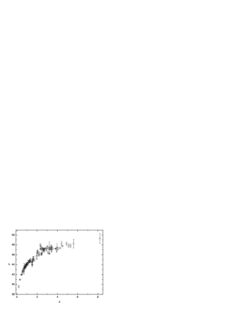
Figure 6: Dispersions of GRBs distance modulus induced by gravitational lensing.

The random magnification of distant sources by the gravitational lensing induces some bias in the observed sample. We calculated the magnification bias as follows. Once the distribution $p(\tau)$ of magnification factor $\tau$ is computed, the magnification bias is drawn from the distribution $p(\tau)$. The dispersion of distance modulus by the gravitational lensing is $\Delta\mu=-2.5$Log$\tau$. In Fig.6 we show the dispersions of the GRB distance modulus induced by the gravitational lensing. We can derive the likelihood function from Bayes’ rule (e.g., Gregory 2005). For each point in a cosmological parameter space, the likelihood function is determined by convolving the distribution of $\tau$ with the intrinsic dispersion distribution (Dodelson & Vallinotto 2006). We used $h=0.742\pm 0.036$ in our calculation (Riess et al. 2009).

4.1 The $\Lambda$CDM cosmology

The luminosity distance in a Friedmann-Robertson-Walker (FRW) cosmology with mass density $\Omega_{M}$ and vacuum energy density (i.e., the cosmological constant) $\Omega_{\Lambda}$ is (Carroll, Press & Turner 1992)

$$d_{L} = c(1+z)H_{0}^{-1}|\Omega_{k}|^{-1/2}{\rm sinn}\{|\Omega_{k}|^{1/2}$$ (20)

$$\times\int_{0}^{z}dz[(1+z)^{2}(1+\Omega_{M}z)-z(2+z)\Omega_{\Lambda}]^{-1/2}\}.$$

We used the GRB sample to constrain the cosmological parameters. Fig.7 shows the $1\sigma$ to $3\sigma$ contour plotting in the $\Omega_{M}-\Omega_{\Lambda}$ plane. The black line contours from 116 GRBs show $\Omega_{M}=0.30_{-0.10}^{+0.09}$ and $\Omega_{\Lambda}=0.84_{-0.78}^{+0.30}$ ($1\sigma$). The dashed contours from 116 GRBs including gravitational lensing magnification bias show $\Omega_{M}=0.26_{-0.09}^{+0.10}$ and $\Omega_{\Lambda}=0.87_{-0.72}^{+0.26}$ ($1\sigma$). From the two contours we can see that the gravitational lensing biases the constraints on cosmological parameters. Because the solid line in Fig.7 represents a flat universe, our result agrees with a flat universe. The contours of GRBs at higher redshifts are almost vertical to the $\Omega_{M}$ axis because the cosmology is matter-dominated at high redshifts.

Figure 7: Confidence contours of likelihood from $1\sigma$ to $3\sigma$ in the $\Lambda$CDM model. The solid-line and dotted-line contours from 116 GRBs without and with the magnification bias.

4.2 The $w(z)=w_{0}$ model

We consider an equation of state for dark energy

$$w(z)=w_{0}.$$ (21)

In this dark energy model, the luminosity distance for a flat universe is (Riess et al. 2004)

$$d_{L}=cH_{0}^{-1}(1+z)\int_{0}^{z}dz[(1+z)^{3}\Omega_{M}+(1-\Omega_{M})(1+z)^{3(1+w_{0})}]^{-1/2}.$$ (22)

Fig.8 shows the constraints on $w_{0}$ versus $\Omega_{M}$ in this dark energy model. The black solid line contours give constraints from 116 GRBs and we have $\Omega_{M}=0.29_{-0.28}^{+0.23}$($1\sigma)$ and $w_{0}=-1.1$. The dashed contours give constraints from 116 GRBs including a gravitational lensing magnification bias: $\Omega_{M}=0.26_{-0.25}^{+0.18}$($1\sigma)$ and $w_{0}=-1.05_{-2.03}^{+0.80}$.

Figure 8: Same as Fig.7 but in $w(z)=w_{0}$ model.

5 Model-independent constraints on the dark energy equation of state

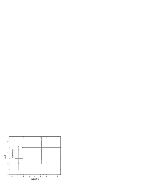
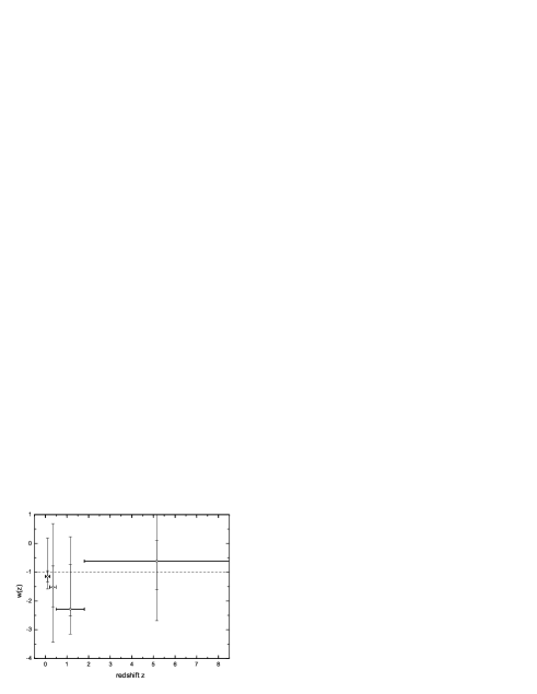
Figure 9: Estimates of the uncorrelated dark energy EOS parameters $w(z)$. Top: uncorrelated dark energy parameters versus redshift, in which the vertical errorbars correspond to $1\sigma$ and $2\sigma$ confidence levels of $w(z)$ and the horizontal errorbars span the corresponding redshift bins. Bottom: Same as top panel but including the weak lensing effect.

We first briefly describe a model-independent method to constrain the equation of state (EOS) (for more details, see Qi, Wang & Lu 2008a). We adopt the redshift binned parametrization for the dark energy EOS as proposed in Huterer & Cooray (2005), in which the redshifts are divided into several bins and the dark energy EOS is taken to be constant in each redshift bin but can vary from bin to bin. For this parametrization, $f(z)$ takes the form (Sullivan et al. 2007)

$$f(z_{n-1}<z\leq z_{n})=(1+z)^{3(1+w_{n})}\prod_{i=0}^{n-1}(1+z_{i})^{3(w_{i}-w_{i+1})},$$ (23)

where $w_{i}$ is the EOS parameter in the $i^{\mathrm{th}}$ redshift bin defined by an upper boundary at $z_{i}$, and the zeroth bin is defined as $z_{0}=0$. This parametrization scheme assumes less about the nature of the dark energy, especially at high redshift, compared with other simple parameterizations, because independent parameters are introduced in every redshift range and it could, in principle, approach any functional form with increasing the number of redshift bins (of course, we would need enough observational data to constrain all parameters well). For a given set of observational data, the parameters $w_{i}$ are usually correlated with each other, i.e. the covariance matrix

$$\textbf{C}=\langle\textbf{w}\textbf{w}^{\mathrm{T}}\rangle-\langle\textbf{w}\rangle\langle\textbf{w}^{\mathrm{T}}\rangle,$$ (24)

is not diagonal. In the above equation, w is a vector with components $\widetilde{w_{i}}$ and the average is calculated by letting w run over the Markov chain. A new set of dark energy EOS parameters $\widetilde{w_{i}}$ defined by

$$\widetilde{\textbf{w}}=\textbf{T}\textbf{w}$$ (25)

is introduced to diagonalize the covariance matrix. The transformation of T advocated by Huterer & Cooray (2005) has the advantage that the weights (rows of T) are positive almost everywhere and localized fairly well in redshift, which facilitates an interpretation of the uncorrelated EOS parameters $\widetilde{w_{i}}$. The evolution of the dark energy with respect to the redshift can be estimated from these decorrelated EOS parameters. The transformation of T is determined as follows. First, we define the Fisher matrix

$$\textbf{F}\equiv\textbf{C}^{-1}=\textbf{O}^{\mathrm{T}}\Lambda\textbf{O},$$ (26)

where O is orthogonal matrix and $\Lambda$ is diagonal. Then the transformation matrix T is given by

$$\textbf{T}=\textbf{O}^{\mathrm{T}}\Lambda^{\frac{1}{2}}\textbf{O},$$ (27)

except that the rows of the matrix T are normalized such that

$$\sum_{j}T_{ij}=1.$$ (28)

In addition to the Union2 SNe Ia sample and 116 GRBs, we also used the distance ratio $D_{V}(0.35)/D_{V}(0.2)=1.736\pm 0.065$ from SDSS7 data (Percival et al. 2010) and the shift parameter $R=1.725\pm 0.018$ from the WMAP seven-year data (Komatsu et al. 2010). The four redshift bins are $0-0.2$, $0.2-0.5$, $0.5-1.8$ and $1.8-8.5$. We marginalize over Hubble parameter $H_{0}$, assuming a broad uniform prior over the range $50<H_{0}<85$ km s^-1 Mpc^-1. We also marginalize over $\Omega_{M}$ assuming the quoted prior from Komatsu et al. (2010). Fig. 9 shows the constraints on EOS $w(z)$. This is the first time that the EOS is constrained beyond the redshift $1.7$. From this figure we can conclude that even though the EOS deviates from $\Lambda$ at $1\sigma$ confidence level, it agrees with $w=-1$ at a $2\sigma$ confidence level.

6 Discussion and conclusions

We have presented the gravitational lensing effects on constraints of cosmological parameters and dark energy from GRBs. We mainly focussed on the non-Gaussian nature of magnification probability distribution functions and the magnification bias of gravitational lensing. We first used an SNe Ia sample to calibrate the luminosity relations of GRBs. Because the luminosity distances of SNe Ia are completely cosmological-model-independent, the GRB luminosity relations can be calibrated in a cosmology-model-independent way. Then we calculated the PDFs of gravitational lensing. The probability distribution functions at high redshifts have higher variance and a lower height of the maximum. The peaks reduce to a smaller magnification factor $\tau$. From the probability distribution functions we can see that the gravitational lensing is more important for high-redshift objects. Finally we presented constraints on cosmological parameters and dark energy. We found that the gravitational lensing had non-negligible effects on the determination of cosmological parameters and dark energy. The gravitational lensing shifts the best-fit constraints of cosmological parameters and dark energy. Because high-redshift GRBs are more likely to be reduced, the most probable value of the observed matter density $\Omega_{M}$ is slightly lower than its actual value. The gravitational lensing also biases a more negative value of the dark energy equation of state. We also constrained the dark energy equation of state out to redshift $z\sim 8$ in a model-independent way using GRBs for the first time, and found that the equation of state deviates from $\Lambda$CDM at the $1\sigma$ confidence level, but agrees with $w=-1$ at a $2\sigma$ confidence level.

As shown in Samushia & Ratra (2010), the cosmological constraints from the two methods of Schaefer (2007) and Wang (2008) may be different when using 69 GRBs. Therefore we emphasize that we need detailed studies of new correlations with a much greater number of GRBs and an examination of systematic errors to be able to regard GRBs as more accurate standardizable candles. Now ongoing missions like Swift, Fermi and Suzaku, and the collaboration of many observers on ground will promise the progression of GRB cosmology.

Appendix A Calculation of the lensing power spectrum

The linear matter power spectrum $\Delta^{2}_{L}(k,z)$ is parameterized as

$$\Delta^{2}_{L}(k,z)=Ak^{n_{s}+3}T^{2}(k)D^{2}(z),$$ (29)

where $D(z)=g(z)/(1+z)g(0)$ is the linear growth factor, $T(k)$ is the transfer function, $A$ is the normalization factor and $n_{s}$ is the primordial fluctuation spectrum. We use the Harrison-Zel’dovich spectrum $n_{s}=1$ throughout. For the $\Lambda$CDM model ($w=-1$), the relative growth factor $g(z)$ is well approximated by (Carroll et al. 1992)

$$g_{\Lambda}(z)=\frac{(5/2)\Omega_{M}(z)}{\Omega_{M}^{7/4}(z)-\Omega_{\Lambda}(z)+(1+\Omega_{M}(z)/2)(1+\Omega_{\Lambda}(z)/70)},$$ (30)

with

$$\Omega_{M}(z)=\frac{\Omega_{M}(1+z)^{3}}{\Omega_{M}(1+z)^{3}+\Omega_{\Lambda}},\ \Omega_{\Lambda}(z)=\frac{\Omega_{\Lambda}}{\Omega_{M}(1+z)^{3}+\Omega_{\Lambda}}.$$ (31)

For the transfer function, we adopt the fitting result of Bardeen et al. (1986) for an adiabatic $\Lambda$CDM model

$$T_{\Lambda}(q)=\frac{\ln(1+2.34q)}{2.34q}[1+3.89q+(16.1q)^{2}+(5.46q)^{3}+(6.71q)^{4}]^{-1/4},$$ (32)

where $q=k/h\Gamma$, and $h=H_{0}/(100\,{\rm km}\,{\rm s}^{-1}\,{\rm Mpc}^{-1})$,and $\Gamma=\Omega_{M}h\exp[-\Omega_{b}(1+\sqrt{2h}/\Omega_{M})]$ is the shape parameter with baryon density $\Omega_{b}$.

For the non-linear power spectrum we adopt the formula given by Peacock & Dodds (1996),

$$\Delta_{NL}^{2}(k_{NL}) = f_{NL}[\Delta_{L}^{2}(k_{L})],$$

$$k_{L} = [1+\Delta_{NL}^{2}(k_{NL})]^{-1/3}k_{NL},$$

$$f_{NL}(x) = x\left[\frac{1+B\beta x+(Ax)^{\alpha\beta}}{1+[(Ax)^{\alpha}g^{3}(z)/(Vx^{1/2})]^{\beta}}\right]^{1/\beta}.$$ (33)

The parameters in the non-linear function $f_{NL}$ are

$$A = 0.428(1+n_{s}/3)^{-0.947},$$

$$B = 0.226(1+n_{s}/3)^{-1.778},$$

$$\alpha = 3.310(1+n_{s}/3)^{-0.244},$$

$$\beta = 0.862(1+n_{s}/3)^{-0.287},$$

$$V = 11.55(1+n_{s}/3)^{-0.423},$$

which are fitted to the numerical simulation results.