Distributed Source Localization in Wireless Underground Sensor Networks

Abstract

Node localization plays an important role in many practical applications of wireless underground sensor networks (WUSNs), such as finding the locations of earthquake epicenters, underground explosions, and microseismic events in mines. It is more difficult to obtain the time-difference-of-arrival (TDOA) measurements in WUSNs than in terrestrial wireless sensor networks because of the unfavorable channel characteristics in the underground environment. The robust Chinese remainder theorem (RCRT) has been shown to be an effective tool for solving the phase ambiguity problem and frequency estimation problem in wireless sensor networks. In this paper, the RCRT is used to robustly estimate TDOA or range difference in WUSNs and therefore improves the ranging accuracy in such networks. After obtaining the range difference, distributed source localization algorithms based on a diffusion strategy are proposed to decrease the communication cost while satisfying the localization accuracy requirement. Simulation results confirm the validity and efficiency of the proposed methods.

I Introduction

Wireless underground sensor networks (WUSNs) are an important extension of terrestrial wireless sensor networks, as they can be used to estimate the location of earthquake epicenters, underground explosions, microseismic activities in mines, etc. Normally, the sensor nodes in WUSNs are buried underground and they exchange information wirelessly via the dispersive underground channel. Some experimental results with WUSNs are reported in [5].

In terrestrial wireless sensor networks, time difference of arrival (TDOA) measurements are widely used for node localization [1]. Because of the physical characteristics of the dispersive underground channel and the heterogeneous network architecture of WUSNs, source localization for WUSNs based on TDOA is more challenging [2]. In a dispersive medium, we cannot directly obtain the range differences between the source and sensors from TDOA measurements since the propagation velocity is a function of frequency; different frequency components will have different propagation delays [3].

Determining the location of sensor nodes is important in many practical applications of wireless underground sensor networks. The objective of a positioning system is to determine accurate node locations with low complexity and communication cost. Localization algorithms for traditional terrestrial wireless sensor networks can be classified into two types: range-based methods and range-free methods. Range-based methods usually have higher location accuracy than range-free ones while demanding additional hardware cost [4].

In [6], a distributed TDOA estimation method that relies only on radio transceivers without other auxiliary measurement equipment was presented. Ultra-wideband (UWB) signaling can be used to accurately achieve time of arrival (TOA) or TDOA measurements, which has the advantages of low-cost and penetrating ability, but also has the weakness of short-range. TDOA based algorithms provide high localization accuracy, and represent a practical method for estimating range differences and source positions in WUSNs. However, this method also faces many challenges. In particular, limited range and directionality constraints decrease the accuracy of range difference estimation. We notice that the TDOA can usually be obtained from the measurement of a signal’s phase which is susceptible to phase ambiguity problems. The Chinese remainder theorem (CRT) offers a closed-form analytical algorithm to calculate a dividend from several of its corresponding divisors and remainders, and can be applied to solve the ambiguity problem here. In our ranging application, the remainders in the CRT are the measured “remainder” wavelengths, the divisors are the measuring wavelengths, and the dividend is the range difference to be estimated. However, directly using the CRT is not feasible due to its over-sensitivity to noise, i.e., a small error in a remainder can lead to very large error in the estimated dividend. To avoid this weakness of the CRT, we propose to use a robust Chinese remainder theorem (RCRT) algorithm to estimate the range difference, in which the dividend can still be reconstructed with only a small error if the errors on remainders are bounded within a certain level [7]. As a result, the range differences or TDOAs can be robustly estimated from noisy measurements in WUSNs by using the RCRT.

After obtaining the range differences using the RCRT, we can estimate the source position based on statistical signal processing methods. For traditional terrestrial wireless sensor networks, TDOA based localization algorithms are normally implemented in a centralized way. In the centralized solution, all nodes relay their TDOA measurements to a fusion center, which uses a conventional localization algorithm to obtain the source position, and then sends the global estimate back to every node. This strategy requires a large amount of energy for communications [9] and has a potential failure point (the central node). Distributed strategies are an attractive alternative, since they are in general more robust, require less communications, and allow for parallel processing. To address this limitation of centralized processing, we propose distributed source localization algorithms using a diffusion strategy in this paper. Diffusion algorithms were proposed in [9, 10, 11] and are applicable to distributed implementations since nodes communicate in an isotropic manner with their one-hop neighbor nodes, and no restrictive topology constraints are imposed. Thus, the algorithms are easier to implement and are also more robust to node and link failures. This approach allows nodes to obtain better estimates than they would without cooperation.

The rest of the paper is organized as follows. Section II establishes the mathematical model of the problem, and derives the proposed ranging method based on the RCRT. Section III gives the distributed source localization algorithm based on the diffusion strategy. Simulation results are given in Section IV, and conclusions are drawn in Section V.

II System model and TDOA estimation via the robust CRT

Due to the large attenuations in underground environments, experimental results show that underground to underground (UG2UG) communication is not feasible at the 2.4GHz frequency band [12]. Underground communication becomes practical only at lower frequencies. As reported in [13] and [14], a WUSN system operating at 433MHz with a maximum transmit power of +10dBm usually achieves a communication range of around one meter for UG2UG communication and more than 30m for underground to aboveground (UG2AG) communication. These communication ranges have already exceeded the wavelength of the transmitted signal, which results in phase ambiguity when the distance difference is directly calculated from the phase. In this section, we first propose a method based on the robust CRT to resolve this phase ambiguity when computing the range distance.

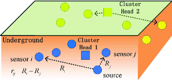
Figure 1: System model for WUSN localization.

Consider a WUSN with $L$ sensor nodes at known positions $({{x}_{i}},{{y}_{i}})$, $i=1,2,\ldots,L$, receiving a signal from a source at an unknown position $(x^{o},y^{o})$ through a dispersive medium, as shown in Fig. 1. The distance between the source and the $i$-th sensor is

$${{R}_{i}}=\sqrt{{{({{x}_{i}}-x^{o})}^{2}}+{{({{y}_{i}}-y^{o})}^{2}}}.$$ (1)

The range difference (RD) between the $i$-th and $j$-th receivers, denoted by ${r_{ij}}$, is ${r_{ij}}={{R}_{i}}-{{R}_{j}}$.

If the medium is non-dispersive, the propagation delay for any frequency is constant. However, in a dispersive medium, the signal propagation velocity is a function of the signal’s frequency, denoted by $v_{k}$ for frequency ${\omega_{k}}$; that is, the propagation delay is frequency dependent. We denote the delay of propagation at frequency $\omega_{k}$ for sensor $i$ as

$${{\tau}_{k,i}}=\frac{{{R}_{i}}}{v_{k}}.$$ (2)

We assume that the source transmits a sinusoid signal ${{s}_{k}}(t)=e^{j\,\omega_{k}t}$ at frequency $\omega_{k}$. The $i$-th sensor receives the signal as

$$\begin{split}{{s}_{k,i}}(t)=e^{j\,\omega_{k}(t-\tau_{k,i})}+n_{i}(t),\end{split}$$ (3)

where $n_{i}(t)$ is the noise at sensor $i$, and $\{{{n}_{i}}(t)\},i=1,2,\ldots,L$ are independent white Gaussian noise processes. Similarly, the received signal at sensor $j$ is

$$s_{k,j}(t)=e^{j\,\omega_{k}(t-\tau_{k,j})}+n_{j}(t).$$ (4)

By taking the cross-correlation of $s_{k,i}(t)$ and $s_{k,j}(t)$, we get

$$I_{k,ij}=\frac{\int^{T}_{0}[s_{k,i}(t)]^{*}s_{k,j}(t)dt}{T}.$$ (5)

It is easy to show that $I_{k,ij}$ is an asymptotically unbiased estimator of $e^{j\omega_{k}(\tau_{k,i}-\tau_{k,j})}$ [17], for which it follows that

$$\lim_{T\rightarrow\infty}\text{E}\{I_{k,ij}\}=e^{j\omega_{k}(\tau_{k,i}-\tau_{k,j})}=e^{j\frac{{{\omega}_{k}}{r_{ij}}}{v_{k}}},$$ (6)

where the range difference $r_{ij}$ is contained in the phase of $I_{k,ij}$. We denote the phase of $I_{k,ij}$ by $\phi_{k,ij}$, i.e.,

$${\phi}_{k,ij}=\left(\frac{{{\omega}_{k}}{r_{ij}}}{v_{k}}\right)\bmod 2\pi.$$ (7)

One can determine ${r_{ij}}$ from ${\phi}_{k,ij}$. However, there are two issues of concern with this approach: 1) the value of ${\phi}_{k,ij}$ is folded by $2\pi$ and 2) the measurements are noisy, i.e.,

$$\frac{{{\omega}_{k}}{r_{ij}}}{v_{k}}={\phi}_{k,ij}+2\pi b_{k}+\nu_{k},$$ (8)

where $b_{k}$ is the quotient (folding integer) and $\nu_{k}$ is the noise at frequency ${{\omega}_{k}}$.

For issue 1, since ${\phi}_{k,ij}\in[0,2\pi)$, no matter how large the actual ${r_{ij}}$ is, the RD ${r_{k,ij}}={\phi}_{k,ij}\cdot v_{k}/{{\omega}_{k}}$ converted directly from ${\phi}_{k,ij}$ is always within one wavelength of the signal, which is ${{\lambda}_{k}}=2\pi v_{k}/{{\omega}_{k}}$. Therefore, $r_{ij}$ cannot be determined uniquely from a single $\phi_{k,ij}$. We add more constraints to confine the solution space by measuring the phase at different frequencies, $\omega_{k},k=1,2,\ldots,K$. The Chinese remainder theorem (CRT) provides a solution to evaluate a dividend from its remainders. We can regard ${r_{ij}}$ as the dividend, ${{\lambda}_{k}}$ as the divisor, and ${r_{k,ij}}$ as the corresponding remainder, i.e.,

$${r_{ij}}=b_{k}{\lambda}_{k}+{r_{k,ij}}.$$ (9)

CRT tells that a positive integer $r_{ij}$ can be uniquely reconstructed from its remainders $r_{k,ij}$ modulo $K$ positive integers $\lambda_{k}$, if $r_{ij}<\text{lcm}\{\lambda_{k}\},k=1,...,K$, where lcm$\{\cdot\}$ denotes least common multiple. It seems that the CRT gives a perfect solution to this problem. However, when we consider measurement noise, the traditional CRT [16] is not suitable because it is sensitive to noise. A small error in the remainder can result in a large error in the estimated dividend. Therefore, we adopt a robust CRT method [7]. Theorem 1 in [7] proves that the robust CRT can tolerate an error in ${r_{k,ij}}$ that is bounded by $\upsilon<B/4$, where $B$ is the greatest common divisor (GCD) among the divisors. To be more specific, if all the remainder errors are not greater than the error bound $\upsilon$, the estimation error of the unknown dividend is upper bounded by $\upsilon$, i.e.

$$\left|r_{ij}-\hat{r}_{ij}\right|\leq\upsilon.$$ (10)

Based on this robust CRT, we provide the following solution to solve the problem:
Step 1. Estimate ${\phi}_{k,ij}$ by calculating the phase of $I_{k,ij}$. Denote the estimated phase by ${\tilde{\phi}}_{k,ij}\in[0,2\pi)$, and the corresponding distance converted from the phase by

$${{\tilde{r}_{k,ij}}}=\frac{{{{\tilde{\phi}}}_{k,ij}}}{2\pi}{{\lambda}_{k}},\quad\text{where }{{\tilde{r}_{k,ij}}}\in[0,{{\lambda}_{k}}),k=1,...,K.$$ (11)

Note that the CRT is commonly expressed over the ring of integers while the distance is a real number. Therefore, we extend the algorithm from the integers to the reals by introducing a real common factor among the divisors as in [18]. We choose those communication frequencies so that the ${{\lambda}_{k}},k=1,...,K$, have a real common factor of $B$ which satisfies

$${{\lambda}_{k}}=B{\Gamma}_{k},$$ (12)

where ${{\Gamma}_{k}}$ are co-prime integers, i.e., $\left({{\Gamma}_{m}},{{\Gamma}_{n}}\right)=1$, for $1\leq m,n\leq K,m\neq n$, and $\left(\cdot,\cdot\right)$ denotes GCD. According to the prior discussion, we have the following equation:

$$\begin{split}{r_{ij}}&={{b}_{k}}{{\lambda}_{k}}+{{r}_{k,ij}}\,\,\,\,,k=1,...,K,\\ &={{b}_{k}}{{\lambda}_{k}}+{{{\tilde{r}}}_{k,ij}}+\Delta{{r}_{k,ij}}\end{split}$$ (13)

where $\Delta{{r}_{k,ij}}$ denotes the measurement errors of ${{\tilde{r}}_{k,ij}}$ with $\left|\Delta{{r}_{ij}^{k}}\right|<\upsilon$, and $\upsilon$ is the error bound.
Step 2. For notational convenience, define the following symbols:

$$\Gamma\triangleq\prod\limits_{k=1}^{K}{{{\Gamma}_{k}}},$$ (14)

$${{\gamma}_{k}}=\Gamma/{{\Gamma}_{k}}.$$ (15)

Calculate and find the sets,

$${{S}_{k}}\triangleq\left\{({{{\bar{b}}}_{1}},{{{\bar{b}}}_{k}})=\arg\underset{({{{\hat{b}}}_{1}},{{{\hat{b}}}_{k}})\in{{\Omega}_{k}}}{\mathop{\min}}\,\left|{{{\hat{b}}}_{k}}{{\lambda}_{k}}+{{{\tilde{r}}}_{k,ij}}-{{{\hat{b}}}_{1}}{{\lambda}_{1}}-{{{\tilde{r}}}_{1,ij}}\right|\right\},k=2,3,...,K,$$ (16)

where

$${{\Omega}_{k}}\triangleq\left\{({{{\hat{b}}}_{1}},{{{\hat{b}}}_{k}})|0\leq{{{\hat{b}}}_{1}}\leq{{\gamma}_{1}}-1,0\leq{{{\hat{b}}}_{k}}\leq{{\gamma}_{k}}-1\right\}$$ (17)

is the solution space of the quotients.

The set $S_{k}$ can be regarded as the optimal combination of the quotients $b_{1}$ and $b_{k}$ with which the difference of the estimated dividends achieves its minimum.
Step 3. Let $S_{k,1}$ denote the first element ${{\bar{b}}_{1}}$ of the 2-tuples,

$$S_{k,1}\triangleq\{{{\bar{b}}_{1}}|({{\bar{b}}_{1}},{{\bar{b}}_{k}})\in{{S}_{k}}\ \textrm{for some}\ {{\bar{b}}_{k}}\}.$$ (18)

Calculate the intersection set of ${{S}_{k,1}}$:

$$S\triangleq\bigcap\limits_{k=2}^{K}{{{S}_{k,1}}}.$$ (19)

In [7], it was proved that if the error bound is less than $B/4$, the set $S$ contains only the true value of ${{b}_{1}}$, i.e., $S=\{{{b}_{1}}\}$. In addition, $b_{k}$ can also be determined from $S_{k}$, that is, if $({{b}_{1}},{{\bar{b}}_{k}})\in{{S}_{k}}$, then ${{\bar{b}}_{k}}={{b}_{k}}$ for $2\leq k\leq K$. Therefore, with all the quotients being determined correctly, the error of the estimated ${r_{ij}}$ is therefore bounded by (10), where $\hat{r}_{ij}$ is obtained by averaging the estimates corresponding to different wavelengths, i.e.,

$${{\hat{r}}_{ij}}=\frac{1}{K}\sum\limits_{k=1}^{K}{({{b}_{k}}{{\lambda}_{k}}+{{{\tilde{r}}}_{k,ij}})}.$$ (20)

Remark: One may notice that to find the set $S_{k}$ in (16) we need to search among the possible values of $\Omega_{k}$, which is a 2-D search problem with the order of $(\Gamma_{2}\Gamma_{3}...\Gamma_{K})^{2}$ and requires a high computational complexity. However, the complexity can be decreased by using a fast algorithm proposed in [7] and [8] to a 1-D search problem with the order of only $2(L-1)\Gamma_{i}$. One can easily apply the fast algorithm to the application in this paper. We do not describe this fast algorithm herein since this is not the focus of this paper.

III Diffusion Algorithms for Source Localization

After obtaining the range differences using the RCRT, a localization algorithm can be used to estimate the source position. Herein, we propose an algorithm for source localization that employs diffusion strategies proposed in [9, 10, 11]. First, the nodes in a cluster send their measurements to the cluster head. Then, the cluster head determines a local estimate using these measurements locally. After obtaining the local estimates, cluster heads exchange their local estimates to achieve diffusion. Before describing the distributed diffusion process, we first discuss the global WLS estimate when all measurements are sent to a fusion center for estimating the source location.

III-A Global Weighted Least Squares Problem

Consider a set of $N$ cluster heads and $K=MN$ sensor nodes (each cluster head is associated with $M$ sensor nodes) spatially distributed over some region with known locations $x_{i}$’s (we consider the 2-D Cartesian coordinate system). The objective of the network is to collectively estimate an unknown deterministic column vector - the location $x$ of a source. All the nodes (cluster heads and sensor nodes) in the network can measure the signal transmitted from the source. The sensor nodes transmit their measurements to the corresponding cluster head and each cluster head forms a set of $M$ TDOA measurements with itself being the reference. Then, cluster heads can send their TDOA measurements to the fusion center. The TDOA measurements are formed one at a time by comparing the signal from the cluster head and the signal from a sensor node, thus leading to uncorrelated estimates if the estimation period is longer than the typical coherence time of the mobile radio channel. Finally, the fusion center obtains altogether $K$ TDOA based range difference measurements $r_{i,j}$’s in the network.

The scalar model for TDOA based range difference is given by

$$r_{i,j}=\|x-x_{i}\|-\|x-x_{j}\|+n_{i,j},$$ (21)

stack all the $r_{i,j}$’s into a vector and write

$$r=s(x)+n$$

where $t=\mathrm{col}\{r_{i,j}\}$, $s(x)=\mathrm{col}\{\|x-x_{i}\|-\|x-x_{j}\|\}$ and $n=\mathrm{col}\{n_{i,j}\}$. Each $r_{i,j}$ can be alternatively denoted as $[r]_{l}$ to reflect its location in vector $r$. The corresponding covariance matrix for $n$ is denoted as $W$ and $W=\mathrm{diag}\{\sigma_{1}^{2},\dots,\sigma_{K}^{2}\}$.

The global weighted least squares estimator for estimating $x$ given $t$ is thus

$$\hat{x}_{G}=\arg\min(r-s(x))^{T}W^{-1}(r-s(x))$$

$$\ \ \ \ =\arg\min\sum_{i=1}^{K}\sigma_{i}^{2}([r]_{i}-[s(x)_{i}])^{2}.$$ (22)

Assuming the $n_{i,j}$’s are Gaussian, then the covariance of $\hat{x}_{G}$ attains the corresponding CRLB, which is given by [15]

$$\mathrm{cov}(\hat{x}_{G})=(P^{T}W^{-1}P)^{-1}$$ (23)

where

$$[P]_{i,j}=\frac{\partial[s(x)]_{i}}{\partial[x]_{j}}\Big{|}_{x=x_{0}}$$ (24)

and $x_{0}$ denotes the true position of the source.

For the TDOA measurements, $P$ is a $K\times 2$ matrix and the elements of $P$ are given by

$$[P]_{l,1}=\frac{[x_{i}]_{1}-[x]_{1}}{\|x_{i}-x\|}-\frac{[x_{j}]_{1}-[x]_{1}}{\|x_{j}-x\|}\Big{|}_{x=x_{0}},$$

$$[P]_{l,2}=\frac{[x_{i}]_{2}-[x]_{2}}{\|x_{i}-x\|}-\frac{[x_{j}]_{2}-[x]_{2}}{\|x_{j}-x\|}\Big{|}_{x=x_{0}}$$

where we assume $[s(x)]_{l}$ involves nodes (a sensor node and a cluster head) $i$ and $j$.

III-B Local Weighted Least Squares Problem

For each cluster head $k$, it has access to limited data from its neighbors. It can then solve the WLS problem locally as

$$\hat{x}_{k}=\arg\min\sum_{i=1}^{K}c_{i,k}\sigma_{i}^{2}([r]_{i}-[s(x)_{i}])^{2}$$ (25)

where $c_{i,k}$’s are the associated weights for node $k$ and $c_{i,k}=0$ if $[t]_{i}$ is not accessible by node $k$. Let $C$ denote the $K\times N$ matrix with elements $c_{i,k}$. We require $\mathds{1}^{T}C=\mathds{1}^{T}$, where $\mathds{1}$ denotes the $N\times 1$ column vector with unit entries.

A local estimate can also be written as

$$\hat{x}_{k}=(P^{T}W^{-1}C_{k}P)^{-1}P^{T}W^{-1}C_{k}z\triangleq L_{k}z$$ (26)

where $C_{k}=\mathrm{diag}\{Ce_{k}\}$ ($e_{k}$ is an $N\times 1$ vector with a unity entry in position $k$ and zeros elsewhere) and $z=r-s(x)+Px|_{x=x_{0}}$. $P$ can be estimated at $\hat{x}_{k}$.

The covariance matrix associated with $\hat{x}_{k}$ is given by $\mathrm{cov}(\hat{x}_{k})=L_{k}WL_{k}^{T}$. Here $L_{k}$ contains only local information due to the selection ability of $C_{k}$.

The estimation fusion method can then be used to fuse these local estimates in a distributed manner by utilizing the local covariance matrices as proper weights and the estimation fusion method can be shown to achieve the performance of the global estimation. However, it involves covariance estimation and matrix inversion.

III-C Diffusion Algorithm

Besides estimator fusion, we can also use a diffusion algorithm to perform distributed estimation. For each cluster head $k$, at the $i$th time epoch, it exchanges its local estimate with its neighboring cluster heads and updates its local estimate using a diffusion algorithm:

$$\hat{x}_{k,i}=\sum_{l=1}^{N}a_{l,k}\hat{x}_{l,i},$$ (27)

where the $a_{l,k}$’s are the diffusion coefficients. Eq. (27) can be considered as a weighted average of the local estimates in the neighborhood of node $k$. Assume all the local estimates are unbiased. Then in order for $\hat{x}_{k,i}$ to be unbiased, we require $\mathds{1}^{T}a_{k}=\mathds{1}^{T}$ where $a_{k}=[a_{1,k},\dots,a_{N,k}]^{T}$. The diffusion process is repeated until all the local estimates have converged, i.e., $\|\hat{x}_{k,i+1}-\hat{x}_{k,i}\|\leq\epsilon\ \forall k$, where $\epsilon$ is a (small positive) design parameter.

One possible choice for the weights $a_{l,k}$ is to consider the degree of connectivity, which is

$$a_{l,k}=\left\{\begin{split}&\mathrm{deg}_{l}/\sum_{n\in N_{k}}\mathrm{deg}_{n},&l\in N_{k}\\ &0,&\textrm{otherwise}\end{split}\right.$$ (28)

where $\mathrm{deg}_{l}$ denotes the cardinality of cluster head $l$’s neighbors (also cluster heads) and $N_{k}$ denotes the set of neighboring cluster heads of head $l$. Such choice has been observed to yield good results for the diffusion algorithm in general [9].

However, this method does not consider the reliability of different local estimates. The reliability of a local estimate is reflected in its associated covariance matrix. But estimating the covariance matrix is not an easy task for a nonlinear weighted least-squares estimator (WLSE). Here we propose a method for setting appropriate $a_{l,k}$’s which reflects the reliability of different local estimates to a certain extent without requiring use of the covariance matrices.

Since each local estimate contains certain errors, when sorting them in respective dimensions (each dimension of $\hat{x}_{k}$ is treated separately), the middle ones are more reliable. Therefore, for cluster head $k$, at the $i$th time epoch, it first finds the median $\tilde{x}_{k,i}$ along respective dimensions among its received local estimates $\hat{x}_{l,i}$’s. Then for each obtained local estimate, head $k$ calculates $w^{i}_{l,k}=\exp(-\|\hat{x}_{l,i}-\tilde{x}_{k,i}\|^{2}/\gamma)$ if $l\in N_{k}$. Otherwise, $w^{i}_{l,k}$ = 0. $\gamma$ is a parameter which controls how rapidly the weight decays as $\|\hat{x}_{l,i}-\tilde{x}_{k,i}\|$ grows. The diffusion coefficient $a^{i}_{l,k}$ is then set to

$$a^{i}_{l,k}=w^{i}_{l,k}/\sum_{j\in N_{k}}w^{i}_{j,k}.$$ (29)

Here we explicitly indicate the time epoch of $w^{i}_{l,k}$ and $a^{i}_{l,k}$ in the superscript. It can be seen that the larger the deviation between a local estimate $\hat{x}_{l,i}$ and $\tilde{x}_{k,i}$, the smaller the weight assigned to this local estimate and vice versa. Obviously, $\mathds{1}^{T}a^{i}_{l,k}=\mathds{1}^{T}$.

Another method of interest is to use an optimization technique. That is, to set $a_{l,k}$’s such that the trace of the covariance matrix of $\hat{x}_{k,i}$ is minimized. We start by examining the first time epoch $i=1$. Then, we have

$$\hat{x}_{k,i}=\sum_{l=1}^{N}a^{i}_{l,k}\hat{x}_{l,i}=\sum_{l=1}^{N}a^{i}_{l,k}L_{l,i}z$$ (30)

where we have used (26).

The covariance matrix of $\hat{x}_{k,i}$ is thus given by

$$\mathrm{cov}(\hat{x}_{k,i})=(\sum_{l=1}^{N}a^{i}_{l,k}L_{l,i})W(\sum_{l=1}^{N}a^{i}_{l,k}L_{l,i})^{T}$$ (31)

and its trace is

$$\mathrm{tr}(\mathrm{cov}(\hat{x}_{k,i}))=\sum_{m,n=1}^{N}a^{i}_{m,k}a^{i}_{n,k}\mathrm{tr}(WL_{m,i}^{T}L_{n,i})=(a^{i}_{k})^{T}Qa^{i}_{k}$$ (32)

where $a^{i}_{k}=[a^{i}_{1,k},\dots,a^{i}_{N,k}]^{T}$ and $[Q]_{m,n}=\mathrm{tr}(WL_{m,i}^{T}L_{n,i})$. To be unbiased, we also require $\mathds{1}^{T}a^{i}_{k}=\mathds{1}^{T}$.

Therefore, to find the optimal $a^{i}_{k}$ in the sense of minimizing the diffusion covariance matrix, we need to solve an optimization problem:

$$\hat{a}^{i}_{k}=\arg\min(a^{i}_{k})^{T}Qa^{i}_{k},\ s.t.\ \mathds{1}^{T}a^{i}_{k}=\mathds{1}^{T},\ a^{i}_{k}\geq 0,\ a^{i}_{l,k}=0\ \forall\ l\notin N_{k}.$$ (33)

This problem is convex if $Q\succ 0$ and thus can be solved fast and efficiently.

After determining $\hat{a}_{k}^{i}$ at time epoch $i$, $L_{l,i+1}$ is updated as $L_{l,i+1}=\sum_{l=1}^{N}\hat{a}^{i}_{l,k}L_{l,i}$ and $Q$ will also be updated accordingly. Then the above optimization process can be performed iteratively until estimates converge.

This optimization method can enhance the distributed fusion performance at the cost of slightly higher computational complexity compared with simply setting $a_{l,k}$ according to (28).

To decrease the computational cost, the optimization process can be implemented only once for the first diffusion at each node, and the weight $a_{k}$ remains the same for the latter diffusions. Since after one diffusion, the updated local estimates becomes much less dissimilar and thus the weights will have much less influence on the followed diffusions.

IV Simulation results

In this section, simulation results are given. We first study the ranging performance using the RCRT in Subsection A. Then, the localization accuracy is introduced in Subsection B.

IV-A Ranging Performance

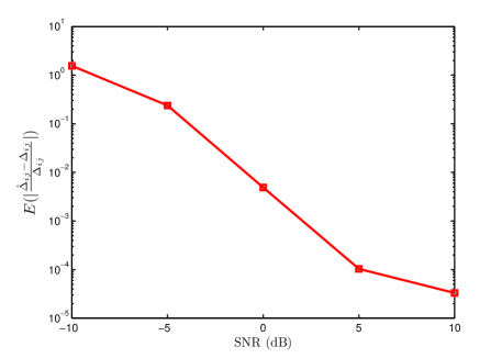
Figure 2: Relative estimation error decreases with increasing SNR.

Assume that the signals are transmitted at 3 frequencies, i.e., $K$=3, $B$=80, ${{\Gamma}_{k}}$=$\{15,16,17\}$, and the corresponding three dividers are $\{1200,1280,1360\}$ which represent the wavelengths ${{\lambda}_{k}}=\{120,128,136\}\text{mm}$. According to the RCRT, the maximum estimation distance is ${{d}_{\max}}=B\prod\limits_{k=1}^{K}{{{\Gamma}_{k}}}$=32640mm. Each trial of simulation generates random integers ${r_{ij}}$, which are uniformly distributed over $[0,{{d}_{\max}}]$. And there are 1000 trials for each SNR. The result is shown in Fig. 2.

Then we consider the effect of $B$ on the performance. We set $B=100,200,300$, respectively and fix ${{\Gamma}_{k}}$=$\text{ }\!\!\{\!\!\text{ 7,9 }\!\!\}\!\!\text{ }$. The result is shown in Fig. 2 with 10000 trials for each SNR. According to the result, changing $B$ does not have significant influence on the relative error of distance estimation.

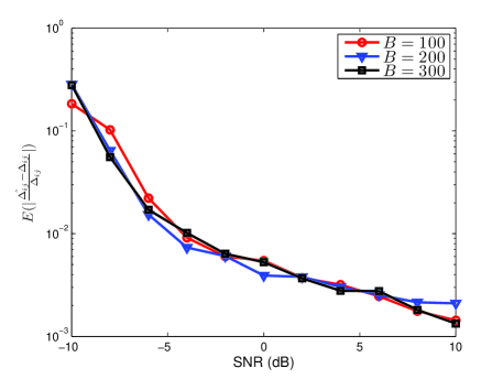
Figure 3: Comparison between the relative estimation errors for different values of $B$.

Next, we compare the performance under different values of $\Gamma_{k}$ with constant $B$ and $K$. In the simulation, we fix $B$=50, $K$=3, and let $\Gamma_{k}$ be $\{7,11,15\}$, $\{29,33,37\}$, $\{53,57,61\}$, respectively. Fig.3 demonstrates that the estimation error increases with ${{\Gamma}_{k}}$. The results from Figs. 2 and 3 can be explained by equations (11) and (12): the phase measurement error is amplified by $B$ and $\Gamma_{k}$, i.e., the error of ${{\tilde{r}}_{k,ij}}$ is $\Delta{{r}_{k,ij}}=\frac{\Delta{{{\tilde{\phi}}}_{k,ij}}}{2\pi}B{{\Gamma}_{k}}$, where $\Delta{{\tilde{\phi}}_{k,ij}}$ denotes the phase measurement error of ${{\tilde{\phi}}_{k,ij}}$. The larger $\Gamma_{k}$ is, the larger error results. However, $B$ does not affect the performance because the robustness of the algorithm also linearly increases with $B$ which cancels the performance deterioration of the increased $B$. (The error tolerance of the algorithm is $\upsilon<B/4$)

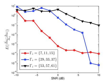
Figure 4: Comparison of the relative estimation error for different values of ${{\Gamma}_{k}}$, when $B$ and $K$ are fixed.

In addition, we consider the scenario in which different sets of $\Gamma_{k}$ are compared under the constraint of constant maximum range ${{d}_{\max}}=B\prod\limits_{k=1}^{K}{{{\Gamma}_{k}}}$. In Fig. 4, We choose ${{\Gamma}_{k}}$=$\{7,11,15\}$, $\{5,11,21\}$, $\{3,11,35\}$, respectively. The simulation results suggest that the performance is better if the differences between the ${{\Gamma}_{k}}$ are smaller.

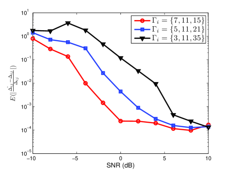
Figure 5: Comparison of the relative estimation error for different values of ${{\Gamma}^{k}}$, with $B$, $K$ and ${{d}_{\max}}$ fixed.

Fig. 5 demonstrates that using more wavelengths results in better ranging performance. In this simulation, we fix the maximum estimation distance ${{d}_{\max}}$, and vary $K$. We consider the cases when $K$=2,3,4, respectively, with $B$=50 and ${{d}_{\max}}$=3465mm. ${{\Gamma}_{k}}$ are set to $\text{ }\!\!\{\!\!\text{ }33,35\text{ }\!\!\}\!\!\text{ }$, $\text{ }\!\!\{\!\!\text{ }7,11,15\text{ }\!\!\}\!\!\text{ }$, $\text{ }\!\!\{\!\!\text{ }3,5,7,11\text{ }\!\!\}\!\!\text{ }$, respectively. Simulation results demonstrate that our RCRT based ranging scheme can estimate the range differences with high accuracy.

IV-B Comparison Results for Distributed Source Localization

We now show simulation results for source localization. The algorithms compared are: 1) Global: the global weighted least square estimator (III-A), 2) Diff (con): the diffusion algorithm with coefficients set by considering connectivity (28), 3) Diff (wei): the diffusion algorithm with coefficients set by weighting (29), 4) Diff (opt): the diffusion algorithm with coefficients set by optimization (33) and 5) Local: simple average of all the local estimates, i.e., $\sum_{k=1}^{N}\hat{x}_{k}/N$.

The root mean square error (RMSE) is used as a performance metric, which is defined as $\sqrt{E(\|\hat{x}-x\|^{2})}$. The Cramer-Rao Lower Bound (CRLB) on the RMSE based on the entire data (equals to $\sqrt{\mathrm{tr}(\mathrm{cov}(\hat{x}_{G}))}$ for Gaussian measurement noise) is also presented as a benchmark. Each simulated point is averaged over 200 runs.

The simulated network consists of $N$ cluster heads that are regularly deployed at grid points. The distance between neighboring cluster heads is set to 50 (the units are meters, here and below). Each cluster head has $M$ associated sensor nodes which are distributed uniformly around the corresponding cluster head. The source location is fixed at $[60,70]$ in all the simulations. The TDOA measurements are generated according to (21) with $n_{i,j}$’s being Gaussian noises. $W$ is set to $W=\sigma^{2}I$ with $\sigma=1$. $\gamma$ is set to 1. The initial point for the WLSE is always set as the center of the deployment area.

Here we consider the scenario in which each cluster head exchanges its local measurements with its neighboring cluster heads to perform a local estimate, and then exchanges its local estimate with its neighboring cluster heads to perform diffusion until convergence. $C$ is set to

$$c_{i,k}=\left\{\begin{split}&\check{c}_{l,k},&[t]_{i}\textrm{ involves cluster head }l,l\in N_{k}\textrm{ and }l\neq k\\ &\check{c}_{k,k},&[t]_{i}\textrm{ involves cluster head }k\\ &0,&\textrm{otherwise}\end{split}\right.$$ (34)

where

$$\check{c}_{l,k}=\left\{\begin{split}&1/\max\{\mathrm{deg}_{l},\mathrm{deg}_{k}\},&l\in N_{k},\ l\neq k\\ &1-\sum_{l\neq k}\check{c}_{l,k},&l=k\\ &0,&\textrm{otherwise}.\end{split}\right.$$ (35)

Here, $\check{c}_{l,k}$ denotes the weight assigned with respect to cluster heads $l$ and $k$, and $c_{i,k}$ represents the weight assigned to the $i$th measurement used by the cluster head $k$.

First, we fix $N=16$ and vary the value of $M$, which changes from 5 to 50 with a step size of 5. The RMSEs of respective algorithms are shown in Fig. 7. It can be observed that Global is the best which can attain the CRLB, local is the worst and Diff (con) is always better than local. In general, Diff (opt) is better than Diff (wei), and Diff (wei) is better than Diff (con). The performance improvement of Diff (opt) and Diff (wei) compared with Diff (con) comes from the consideration of the reliability of the local estimates. Though the diffusion algorithms are always worse than Global, the performance differences are not significant. As $M$ grows, all the algorithms perform better.

Fig. 8 shows the corresponding average CPU times of respective algorithms except Diff (opt) whose CPU time is typically 10 times that of Global due to its numerical optimization nature (the same below). It can be seen that Diff (con) is very time efficient with a CPU time almost the same as local. Diff (wei) consumes a little more CPU time than Diff (con), while the CPU time of Global is much larger. This demonstrates the advantage of the diffusion algorithm in terms of CPU time and computational complexity. Furthermore, we can say the diffusion algorithm has lower communication cost and computation complexity than the centralized solution, while the localization accuracy is close to the centralized method.

Fig. 9 shows the average number of iterations before convergence of the three diffusion algorithms. We can observe that Diff (opt) requires many fewer iterations compared with Diff (con) and Diff (wei). Diff (wei) needs slightly more iterations than Diff (con), which may explain our observation of a slightly longer CPU time consumed by Diff (wei).

We now fix $M=10$ and examine the effects of the number of cluster heads $N$ on the performance of the algorithms. We vary $N$ from 4 to 36. The RMSEs of the algorithms are shown in Fig. 10. It is clear that adding more clusters (and thus sensor nodes) will not necessarily improve the estimation performance. This is known as the geometric effect of the localization problem. Since the source location is outside the convex hull formed by respective added clusters, the corresponding local estimates are not good enough. Diff (con) and Diff (wei) thus also show performance degradation. However, Diff (wei) is much better than Diff (con) when more clusters are added while the sensor nodes associated with each cluster head is fixed. The performance of Global is almost unchanged as $N$ becomes large. Due to the consideration of the estimation covariance matrices, Diff (opt) shows very good performance. However, it will consume much more CPU time. The corresponding average CPU times and average number of iterations are shown in Figs. 11 and 12 respectively. Similarly, Diff (con) is the most time efficient and Diff (opt) requires the smallest number of iterations.

Then we examine the effect of $\sigma$ on the performance of the algorithms. We set $N=16$ and $M=10$. The RMSEs of respective algorithms are shown in Fig. 13. The relative performance of respective algorithms is the same as before. As $\sigma$ enlarges, all of them show performance degradation. The average CPU times and average number of iterations among different algorithms have the same relationship as before and thus the figures are not shown here.

Finally, we examine the choice of $\gamma$ on the performance of Diff (wei). We set $N=16$, $M=10$ and $\sigma=1$. We generate 200 realizations of the overall TDOA measurement vector, then store and use them for all the corresponding simulations. The corresponding RMSEs are shown in Fig. 14. It can be seen that an optimal $\gamma$ exists which results in the minimum RMSE for Diff (wei). However, in a large range of the choice of $\gamma$, Diff (wei) can generate better results than Diff (con).

V Conclusion

We have presented energy efficient localization schemes that can achieve high localization accuracy in wireless underground sensor networks. These distributed localization algorithms require low computational complexity and energy consumption based on a diffusion strategy. An accurate RCRT based ranging scheme using TDOA to determine range differences between sensors and source that does not require time synchronization is also proposed. It has been shown via simulation results that the proposed localization algorithms achieve excellent localization accuracy with lower communication cost. In future work, we plan to implement our localization scheme in a testbed and verify its performance with an actual WUSN.

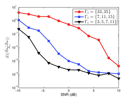
Figure 6: Comparison of the relative estimation error for different values of $K$.

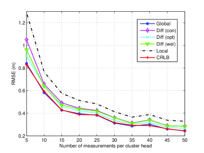
Figure 7: RMSE versus $M$ when $N=16$.

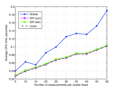
Figure 8: CPU time versus $M$ when $N=16$.

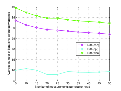
Figure 9: Average number of iterations before convergence versus $M$ when $N=16$.

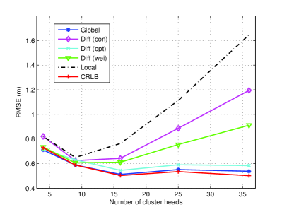
Figure 10: RMSE versus $N$ when $M=10$.

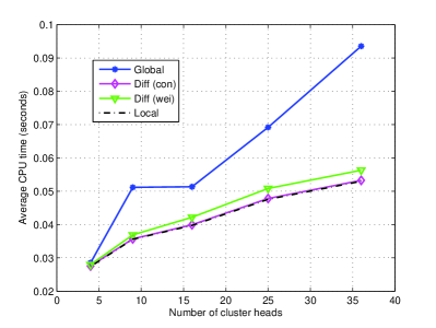
Figure 11: CPU time versus $N$ when $M=10$.

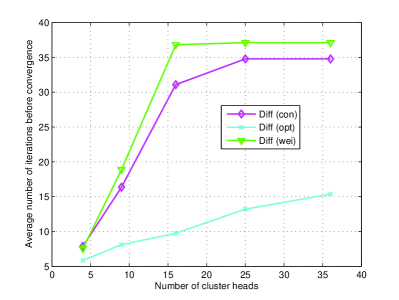
Figure 12: Average number of iterations before convergence versus $N$ when when $M=10$.

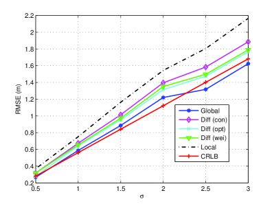
Figure 13: RMSE versus $\sigma$.

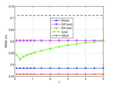
Figure 14: RMSE versus $\gamma$.

References

- [1] J. Luo, H. V. Shukla, and J.-P. Hubaux, “Non-interactive location surveying for sensor neworks with mobility-differentiated ToA,” in Proc. IEEE INFOCOM, Barcelona, Spain, Apr. 2006, pp. 1-12.
- [2] Z. Sun and I. F. Akyildiz, “Connectivity in wireless underground sensor networks,” in Proc. SECON, Boston, Massachusetts, USA, Jun. 2010, pp. 1-9.
- [3] Y.T. Chan, T.K.C. Lo, and H.C. So, “Passive range-difference estimation in a dispersive medium,” IEEE Transactions on Signal Processing, vol. 58, no. 3, pp.1433-1439, March 2010.
- [4] C. Wang, J. Chen, and Y. Sun, “Sensor network localization using kernel spectral regression,” Wireless Communications and Mobile Computing (Wiley), vol. 10, pp. 1045-1054, June 2010.
- [5] A.R. Silva and M.C. Vuran, “Communication with aboveground devices in wireless underground sensor networks: An empirical study,” in Proc. IEEE ICC’10, Cape Town, South Africa, May 2010.
- [6] W. Zhang, Q. Yin, and W. Wang, “Distributed TDoA estimation for wireless sensor networks,” in Proc. ICASSP’10, Dallas, Texas, Mar. 2010, pp. 2862-2865.
- [7] X. Li, H. Liang, and X. Xia, “A robust Chinese remainder theorem with its applications in frequency estimation from undersampled waveforms,” IEEE Transactions on Signal Processing, vol. 57, no. 11, pp. 4314-4322, Nov. 2009.
- [8] G. Li, J. Xu, Y.-N. Peng, and X.-G. Xia, “An efficient implementation of robust phase-unwrapping algorithm,” IEEE Signal Process. Lett., vol. 14, pp. 393-396, Jun. 2007.
- [9] F. S. Cattivelli, C. G. Lopes, and A. H. Sayed, “Diffusion recursive leastsquares for distributed estimation over adaptive networks,” IEEE Trans. on Signal Process., vol. 56, no. 5, pp. 1865-1877, May 2008.
- [10] F. Cattivelli and A. H. Sayed, “Diffusion LMS strategies for distributed estimation,” IEEE Trans. on Signal Process., vol. 58, no. 3, pp. 1035-1048, March 2010.
- [11] C. G. Lopes and A. H. Sayed, “Incremental adaptive strategies over distributed networks,” IEEE Trans. on Signal Process., vol. 55, no. 8, pp. 4064-4077, August 2007.
- [12] E. Stuntebeck , D. Pompili, and T. Melodia, “Underground wireless sensor networks using commodity terrestrial motes,” in Proc. IEEE SECON’06, Reston, USA, Sep. 2006, pp. 112-114.
- [13] A. R. Silva and M. C. Vuran, “Empirical evaluation of wireless underground-to-underground communication in wireless underground sensor networks,” in Proc. DCOSS’09, Marina Del Rey, CA, Jun. 2009, pp. 231-244.
- [14] A. R. Silva and M. C. Vuran, “Development of a testbed for wireless underground sensor networks,” EURASIP Journal on Wireless Communications and Networking, vol. 2010, Article ID 620307, 14 pages, 2010.
- [15] S. M. Kay, Fundamentals of Statistical Signal Processing: Estimation Theory. Englewood Cliffs, NJ: Prentice-Hall, 1993.
- [16] T. Koshy, Elementary Number Theory with Applications, 2nd ed., Burlington, MA: Elsevier, 2007, pp. 295-302.
- [17] J.G. Proakis and M. Salehi, Digital Communications, 5th ed., New York, NY: McGraw-Hill, 2008.
- [18] W. Wang and X.-G. Xia, “A closed-form robust Chinese remainder theorem and its performance analysis,” IEEE Transactions on Signal Processing, vol.58, no.11, pp.5655-5666, Nov. 2010.