Investigation of Residual Blaze Functions in Slit-Based Echelle Spectrograph

Abstract

We have studied the Residual Blaze Functions (RBF) resulting from division of individual echelle orders by extracted flat-field in spectra obtained by slit-fed OES spectrograph of 2m telescope of Ondřejov observatory, Czech Republic. We have eliminated the dependence on target and observation conditions by semiautomatic fitting of global response function, thus getting the instrument-only dependent part, which may be easily incorporated into data reduction pipeline. The improvement of reliability of estimation of continuum on spectra of targets with wide and shallow lines is noticeable and the merging of all orders into the one long spectrum gives much more reliable results.

1 Introduction

The requirement of a modern astrophysical analysis, to study the wide range of the object spectrum in the greatest details, or to observe its variability in many spectral lines at the same time, lead naturally to the usage of cross-dispersed echelle spectrographs.

Although the reduction of the echelle raw frames is quite straightforward and a number of automatic reduction pipelines has been in use for many instruments, there remains still unsolved the problem of the reliable normalization of individual extracted spectral orders before merging into one long continuous spectrum.

Due to its inherent nature the echelle blaze function has to be removed from all orders with the immense precision, otherwise the strong ripple patterns appear on the merged spectrum. They make difficult the fitting of the continuum an hence influence the reliability of the measurement of equivalent widths of wide shallow lines, the placement of wings of hydrogen lines of hot rapidly rotating stars, or the studies of diffuse interstellar bands.

2 Basic Reduction of Echelle Spectra

2.1 Characteristic Features of Echelle Spectrographs

Almost all modern high-dispersion spectrographs used today are the cross-dispersed echelle spectrographs giving the very high angular dispersion and the extensive wavelength coverage at the same time. The individual spectral orders (typically 30 to 100), representing short piece of the spectrum (several tens of Å), are imaged at the rectangular CCD chip as a slanted parallel strips, sometimes even slightly curved. This breeds, however, the large complex of problems concerning the data reduction as the correct echelle data reduction is very sensitive to even very small errors or omissions.

2.2 General Reduction Techniques

The basic principles of the reduction is described in a number of places [1, 2, 3, 4]. There are also detailed cookbooks for reduction using particular package (mainly IRAF[5, 6]).

The general reduction requires a number of steps to remove the detector features as in all CCD processing. Here comes the bias removal and overscan correction and (if necessary) dark current elimination. Then there might follow classical flat-fielding using the original 2-dimensional flat image, but it is generally not done due to problems with blaze function (see later). The quite difficult task in this part is the removal of fringing that disturbs the spectra in the IR region on the thinned chips. The preferred way is the flat-fielding on the extracted 1-dimensional spectra, that also removes the main part of blaze function.

On this cleaned flat field frame the echelle cross-order positions are found by looking through central cut of the frame, perpendicular to dispersion, and then the cross-order centers are traced towards both ends. Then a bilinear polynomials are fitted through all cross-order center positions. In this step the background, containing the scattered light, has to be removed. Sometimes the instrument bias elimination is postponed to this moment. The scattered light can be found by taking the median values of region between echelle orders and fitting a 2-dimensional surface through it, that is then subtracted from the data. Although it might work well for certain instruments with the large gaps between the orders, for the instruments with densely packed orders the physical model of the scattering has to be applied. This is very difficult and computing demanding task [3, 7, 5, 2] but it has great importance even for the very precise space spectrograph STIS [8].

Now it can begin the extraction of the flux from the stellar orders following the traces of cross-order center positions — usually using traces from flat field orders. The extraction is done with the optimal variance-weighted methods [9, 10] eliminating the cosmic rays at the same time. There are still attempts to improve this well-proved algorithms [11].

The critical part is now the wavelength calibration by fitting 2-dimensional polynomials through the measured position of a hundreds of sharp lines of the comparison arc spectrum. The availability of more precise instruments also needs the re-analysis of standard calibration algorithms [12].

Although quite complicated, this part of echelle reduction is quite straightforward and the automatic pipelines can be used to reduce the data. We end up with separate echelle orders with associated wavelength scale.

Such data are very useful for measurement of radial velocities of many lines (used in cross-correlation techniques [13] on late-type stars with many sharp lines) or for study of abundances using the equivalent width of many deep sharp lines of heavy elements [14].

2.3 The Merging of Individual Echelle Orders

The disadvantage of echelle spectra is the very short spectral span of individual orders (typically less than 100 Å). The work on individual orders can be done for late-type stars with narrow lines, where the sufficient pseudo-continuum windows are seen in each order. For hot and rapidly rotating stars, where hydrogen and helium lines are of great interest, the considerably wide line profile is spread over several echelle orders. Therefore the merging of several orders is required to see the whole profile together with the surrounding pseudo-continuum. Although the merging can be done quite easily after rebinning of orders to the same wavelength grid (preferably in $\log\,\lambda$), by weighted averaging of the overlapping regions (and cutting the very edges where the high noise is present), this step requires extremely precise handling of data to get reliable results. The problem is caused by the behavior of the echelle blaze function.

2.4 The Blaze Function

The most serious problem in the reduction, that has not been yet solved satisfactorily, is the removal of the grating blaze function. The blaze function changes the intensity of the spectrum inside each order and thus modulates strongly the shape of the stellar continuum. In each order, the intensity of signal steeply rises from one edge to the center of frame and falls down to the other edge.

2.4.1 Methods of blaze function removal

There are several methods of the blaze function removal. One of the most promising is the model of its theoretical shape. From the diffraction theory the blaze function should behave like a sinc-squared function of the spectrograph construction parameters (the angle of incidence, angle of blaze, grating grooves width and spacing). If knowing these parameters precisely, a model of blaze may be constructed. It is, however, only an approximation, as the real blaze is not produced by an ideal grating, but other construction features have its influence as well.

This method developed by Barker[15] was applied to the high-dispersion spectra from IUE satellite and implemented later by Cassattella in IUE NEWSIPS pipeline. Although it was quite successful as the first approximation of ripple correction and may be used to remove the largest part of intensity modulation before using sophisticated differential methods [16], it will not completely remove the influence of the blaze from data.

Other method is the usage of the spectra of the spectrophotometric standard taken at about the same time as the primary target. The identically processed data of the standard are then divided by its absolute flux and the ratio is used to get the flux of the object. Due to its dependence on the extinction and the requirement of a sufficiently bright standard in the target proximity this method is used mainly in space instruments — e.g. for reducing HST STIS data. Even here some problems with order merging remains[17].

The widely used method at most modern spectrographs is the division by the extracted flat field spectrum. This method should give the best results, mainly for fiber-fed spectrographs, where the cross-order profile of the star and flat is the same, provided that their blaze function is identical. In practice, however, this is not the case, and the blaze function shows small variations of still unknown origin. Some experiments with the fiber-fed spectrographs give clues to the suspicion of the influence of flat-field calibration units and the influence of fiber itself. But some part of the changes is probably intrinsic to the grating theory itself (e.g. polarization change).

There are, thus, attempts to remove the blaze function by fitting the smooth surface through only the extracted stellar data in pixel-order space, using only the orders where the continuum is present. In this case, the flat field is used only for adjusting the CCD pixels sensitivity — first it is smoothed still in original 2-dimensional frame. This method, however, fails in the blue region on the spectra of hot or rapidly rotating stars where almost every order is contaminated by wide Balmer lines.

2.4.2 Blaze function instability

The tiny changes in position of the orders as well as in the cross-order profile shape are commonly observed between flat field and stellar spectrum even in case of the well stabilized instrument in protected environment like FEROS [18] or ELODIE [6].

Corresponding small shift of blaze function then causes the tilt of individual flat-fielded orders and introduces intensity jumps between the overlapping edges of successive orders. If such data is blindly merged uncorrected (as in the automatic pipeline), the strong ripple-shaped periodic undulations with the period corresponding to free spectral range occur on the continuum shape. The extracted flat-field spectra mutually divided show clearly the time-dependent variations of order of several percent. [19]. This behavior is confirmed by our experience with the HEROS and FEROS data as well [20].

The blaze function time-dependent variations were also reported on HST STIS spectrograph by Bowers and Lindler [17]. They have the suspicion, that the blaze changes are caused not by the grating movement but by the changes of the grating surface (size and position of individual grooves).

2.4.3 The influence of the fiber or slit on blaze function

Although the light from the flat field and star goes through the same slit and the same narrow decker, the illumination pattern of the flat is generally different from the stellar one, it changes with the seeing and depends on the precision of the guiding. The influence of these centering errors on radial velocity shifts was studied in detail[16], but it will cause the micro-shifts of the order positions as well. In case of fiber-fed spectrographs this effect should not be present, as is generally believed. There are, however, evidences that it is not true at the level of precision we need.

There has been proved the influence of the optical fiber on the transported light which will slightly change the position of spectral orders on the detector. Even the double fiber scrambler (between the two pieces of chopped fiber are inserted micro-lenses) used for the precise RV measurement (mainly in search for extrasolar planets) does not help to eliminate all the blaze function variations. One of the instruments equipped with the fiber scrambler is ELODIE [21], but spectra from it had to be artificially corrected before merging orders as well [22]. The same problems are present in spectra from more advanced high precision instrument SOPHIE (Ilovaisky 2007, private communication).

2.5 The Problem of Continuum Normalization

Although most of the reduction procedures give quite satisfactory results in blaze function removal, there still remain small systematic errors in the unblazed spectra. An automatic merging of orders then may result in periodic ripple disturbances in the shape of the apparent stellar continuum. A typical way to remove them is the manual fitting of a sufficiently smooth spline function through the parts of the merged spectrum where the continuum seems to be present. However, for the wide lines with large wings it is very difficult to do the normalization by spline interpolation between neighboring continuum windows if the ripples are present.

3 Merging of OES Spectra

3.1 Ondřejov Echelle Spectrograph (OES)

The OES[23] is the slit-fed prism cross-dispersed echelle spectrograph developed at the Stellar department of the Astronomical Institute of the Academy of Sciences of the Czech Republic and installed at the coudè focus of 2m telescope of the Ondřejov observatory. In its current setup it can cover spectral range from 3750Å–9500Å in 62 orders. Due to various construction limitations there is a lack of order overlap at wavelengths longer than about 6000 Å. This together with strongly curved orders, tilted spectral lines and high level of inter-order scattered light makes reduction extremely complicated. Moreover, there is some vignettation seen at the edges of the orders. The example of the echelle-gram is given on the Fig. 1.

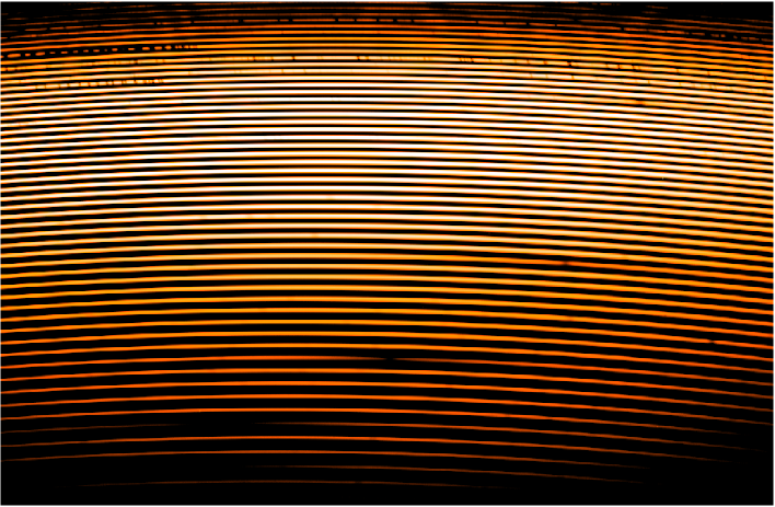
Figure 1: Part of OES echelle-gram of Vega.

3.2 Residual Blaze Function

In general the blaze function of stellar exposures on slit-fed echelle spectrographs is quite different from blaze function of the flat field spectrum due to different character of slit illumination. So the unblazing by direct division of the extracted stellar continuum by the extracted flat field does not remove the shape of blaze function completely and some residual structure remains superimposed on the stellar continuum. For such a curve we are using the term Residual Blaze Function (RBF). In the ideal case it should be the line of constant value corresponding to the ratio of intensity of stellar and flat field exposures. This is better fulfilled by fiber-fed spectrographs as the illumination of flat and star is almost the same due to the same size of fiber entrance with a micro-lens. The example of the behavior of one spectral order on fiber spectrograph HEROS is given on Fig. 2.

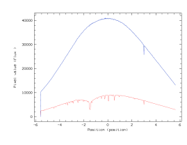
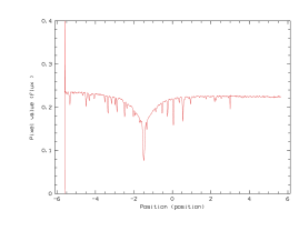
Figure 2: HEROS: Left: Extracted orders of star and flat. Right: Stellar order after division by extracted flat.

However, the shape of such orders in case of OES is more complicated mainly influenced by vignettation due to incompatibility of illumination structure. Examples of orders containing line ${H_{\gamma}}$ and ones with obvious continuum for case of Vega and Arcturus are given on Fig. 3 and Fig. 4.

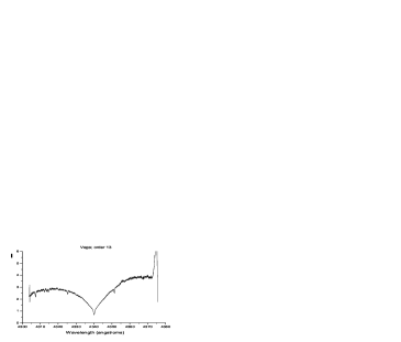
Figure 3: OES: unblazed order 13 with line $H_{\gamma}$. Left: Arcturus. Right: Vega

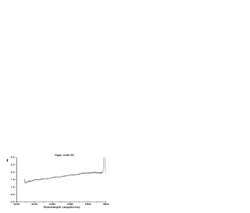
Figure 4: OES: unblazed order 30 with continuum. Left: Arcturus Right: Vega

3.2.1 Estimation of the Residual Blaze Function

As the true RBF is unknown (we do not see the true continuum due to wide lines and blends), we have to estimate its shape using comparison with other spectrum with already known RBF. The best case is the spectrum of the same target with approximately same resolution that is already continuum normalized (the continuum reference spectrum). If the resolution is not similar, the high resolution spectrum has to be convolved with sufficiently wide Gaussian profile to reach comparable lower resolution. One good option is the spectrum from single order spectrograph, where the continuum is easily obtained.

3.2.2 Preparation of continuum normalized reference spectrum

In the ideal case of several bright stars, there are available their normalized merged spectra either in web archives (e.g. ELODIE archive[22]) or published spectral atlases. For our case we used the high resolution atlas of Arcturus by Hinkle et al.[4] and Vega atlas of Takeda et al. [24]

We also tried to rectify the spectra of Vega and Arcturus order by order ourselves to preserve the resolution. The rectification polynomials were applied iteratively in custom program SPEFO[25], checking the consistency of order overlaps and finally comparing visually the merged rectified spectrum with the synthetic spectrum.

We used synthetic stellar spectra with temperatures approximately corresponding to temperature of Arcturus (Teff=4300 K) and Vega (Teff=9300 K). After that we used the ”sYnt-Rotate” command of SPEFO program, where we put corresponding rotation velocity of Arcturus ($v\sin i$=2 km/s) and Vega ($v\sin i$=25 km/s). After required rotational broadening we used those synthetic spectra in further visual comparisons.

3.2.3 Determination of Residual Blaze Function

After dividing non-rectified spectrum (individual orders) of Arcturus and Vega by rectified ones (continuum master reference), we get the shape of residual blaze function for each order. Following figures show comparison of shape of residual blaze functions in two different orders (containing Balmer lines ${H_{\gamma}}$ and ${H_{\beta}}$) of Arcturus and Vega (Fig. 5). The global view of RBFs in all orders can be seen on Fig. 6.

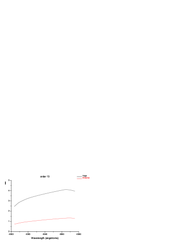
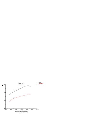
Figure 5: Comparison of RBFs in two orders of Arcturus and Vega. Left: Order 13. Right: Order 22.

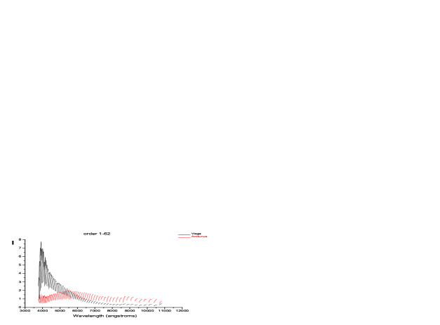
Figure 6: Comparison of global shape of residual blaze functions for Arcturus and Vega.

3.3 The Global Sensitivity Function

As is seen on Fig. 6, the RBFs are following some smooth curve different for Arcturus and the Vega. We suppose that this function, that we call the Global Sensitivity Function (GSF), depends on the ratio of energy distributions of the target and the flat field lamp and on the relative sensitivity of CCD detector in given spectral region.

Given constant source of flat field lamp and the stable CCD detector, we can suppose GSF is only dependent on the target color and extinction (spectral energy distribution- SED). Color changes are expected to be dependent on the extinction and hence the zenith distance of the target, as well as on seeing, atmospheric differential refraction and other observation-dependent parameters. That is the reason why we have chosen Vega and Arcturus as representants of two different SEDs (cold and hot star) and extinction (different zenith distance at the time of observation).

3.3.1 Fitting of global sensitivity function

To find some representative scaling point-to-point on each order one could use the approximate center of each order. We have used, however, the median of distribution of values in every order. The median better represents some “middle” point for case of strongly curved RBF. The orders contaminated by wide Balmer lines have even this estimate wrong, but the remaining points (with possible elimination of known contaminated orders) are easily fitted by smooth polynomial while rejecting deviant points in an iterative procedure (Fig. 7).

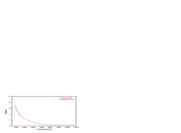
Figure 7: Fit of GSF through median points in Vega orders

The knowledge of target GSF then can prepare rectified individual orders even before merging, but the normalization can be done easily on merged spectrum as well.

3.4 The Intrinsic Residual Blaze Function

Our order correction procedure is based on hypothesis supposing the RBF to be just product of some instrument-dependent part, called Intrinsic Residual Blaze Function (IRBF) and the GSF, which is observation dependent. We can get it from division of RBF by GSF. Example of IRBF for the two orders shown above (see Fig. 5) is given in Fig. 8.

Once known, the IRBF can be divided out from flat-fielded stellar orders (on extracted spectra) and the corrected orders should be matching better thus allowing easy merging of orders. Some examples of this procedure in global and detailed view is given on Fig. 9 and Fig. 10. If the GSF for given observation is estimated, the resulting spectrum should become even continuum normalized (to level 1.0)

Figure 8: Comparison of IRBFs in two orders of Arcturus and Vega. Left: Order 13. Right: Order 22.

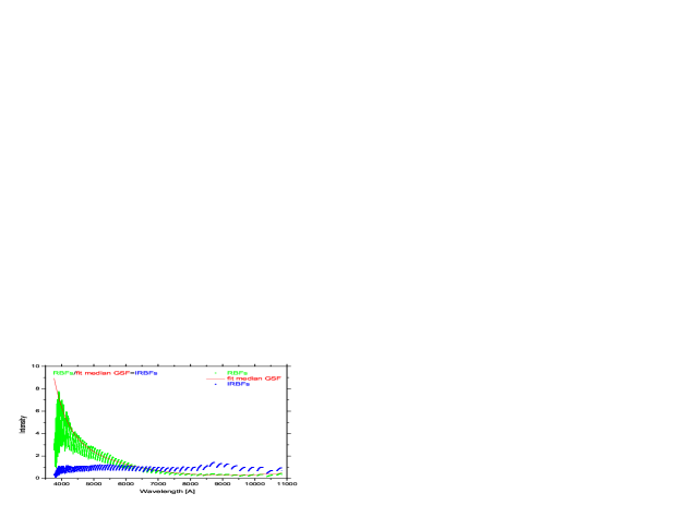
Figure 9: RBF and IRBF of Vega with median fit of GSF

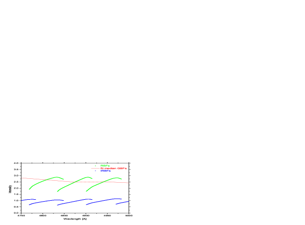
Figure 10: Detail view on RBF and IRBF on Vega with median fit of GSF

3.5 Correction of Flat-Fielded Stellar Orders

The final goal of the reduction process is the continuum normalized (rectified) merged spectrum of a target. If the IRBF is really constant for given spectrograph, we can built it in an reduction pipeline, so every flat-fielded order is divided by it, before merging in one long spectrum (Fig. 11).

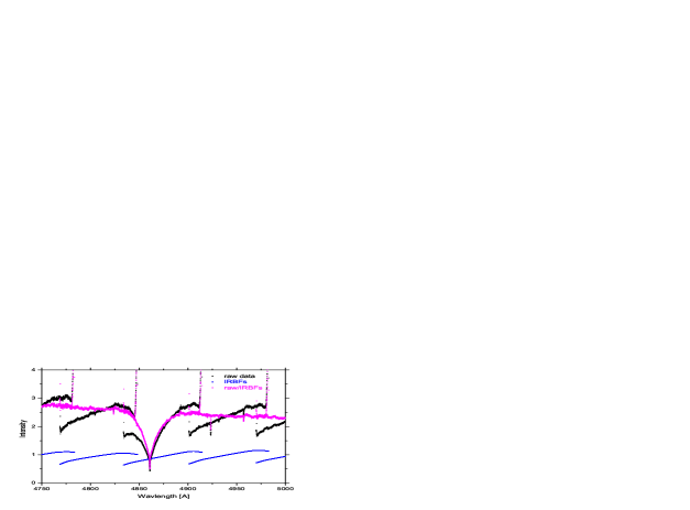
Figure 11: Raw unblazed data after correction by IRBF. Merged profile of ${H_{\beta}}$

This correction will assure the consistent behavior of order edges in the region of overlapping orders and thus smooth connection of neighboring orders together. See Fig. 12 for example of merged Vega orders in different spectral regions.

Figure 12: Merged orders of Vega in different spectral regions. The vertical lines mark the edges of individual orders. Note the gaps in red region. Left: Blue region. Right: Red region.

4 Conclusion

We have shown a one possible way how to tackle the problem of precise unblazing of echelle spectra using the separation of correction function to instrument-only dependent part (IRBF) changing on the scale of one echelle order and observation-dependent part (GSF) smoothly changing over the whole observed spectrum.

Even if this is not the final solution, and still some quickly changing variations remain, the resulting corrected echelle orders may be merged in the one long spectrum much more easily avoiding strong ripples. If the estimate of GSF is known for given observation, the spectra may be normalized to continuum almost automatically.

Our method is just a first simple approximation of the general correction procedure, it may be instrument dependent (better suited to slit-fed spectrographs) and so the future investigation of the problem is still highly desirable.

- [1] Valdes, F., Guide to the Slit Spectra Reduction Task DOECSLIT. NOAO (1993).
- [2] Goodrich, R. W. and Veilleux, S., “Reduction of Hamilton echelle data at Lick Observatory,” PASP 100, 1572–1581 (Dec. 1988).
- [3] Hall, J. C., Fulton, E. E., Huenemoerder, D. P., Welty, A. D., and Neff, J. E., “The reduction of fiber-fed echelle spectrograph data: Methods and an IDL-based solution procedure,” PASP 106, 315–326 (Mar. 1994).
- [4] Hinkle, K., Wallace, L., Valenti, J., and Harmer, D., [Visible and Near Infrared Atlas of the Arcturus Spectrum 3727-9300 A ] (2000).
- [5] Churchill, C. W., “An echelle reduction manual for iraf users,” Tech. Rep. 74, Lick Obs. Tech. Rep (1994).
- [6] Erspamer, D. and North, P., “Automated spectroscopic abundances of A and F-type stars using echelle spectrographs. I. Reduction of ELODIE spectra and method of abundance determination,” A&A 383, 227–238 (Jan. 2002).
- [7] Gehren, T. and Ponz, D., “Echelle background correction,” A&A 168, 386–388 (Nov. 1986).
- [8] Howk, J. C. and Sembach, K. R., “Background and Scattered-Light Subtraction in the High-Resolution Echelle Modes of the Space Telescope Imaging Spectrograph,” AJ 119, 2481–2497 (May 2000).
- [9] Horne, K., “An optimal extraction algorithm for CCD spectroscopy,” PASP 98, 609–617 (June 1986).
- [10] Mukai, K., “Optimal extraction of cross-dispersed spectra,” PASP 102, 183–189 (Feb. 1990).
- [11] Piskunov, N. E. and Valenti, J. A., “New algorithms for reducing cross-dispersed echelle spectra,” A&A 385, 1095–1106 (Apr. 2002).
- [12] de Cuyper, J.-P. and Hensberge, H., “Wavelength calibration at moderately high resolution,” A&AS 128, 409–416 (Mar. 1998).
- [13] Skuljan, J., Hearnshaw, J. B., and Cottrell, P. L., “High-Precision Radial Velocity Measurements of Some Southern Stars,” PASP 112, 966–976 (July 2000).
- [14] Katz, D., Soubiran, C., Cayrel, R., Adda, M., and Cautain, R., “On-line determination of stellar atmospheric parameters T_eff, log g, [Fe/H] from ELODIE echelle spectra. I. The method,” A&A 338, 151–160 (Oct. 1998).
- [15] Barker, P. K., “Ripple correction of high-dispersion IUE spectra - Blazing echelles,” AJ 89, 899–903 (June 1984).
- [16] Verschueren, W., Brown, A. G. A., Hensberge, H., David, M., Le Poole, R. S., de Geus, E. J., and de Zeeuw, P. T., “High S/N Echelle Spectroscopy in Young Stellar Groups. I. Observations and Data Reduction,” PASP 109, 868–882 (Aug. 1997).
- [17] Bowers, C. and Lindler, D., “Stis echelle blaze shift correction,” in [2002 HST Calibration Workshop ], 127–136, Space Telescope Science Institute (2002).
- [18] Hensberge , H., “Evaluation of FEROS pipeline,” tech. rep., ESO (2002). http//www.ls.eso.org/lasilla/Telescopes/2p2T/E1p5M/FEROS/Reports/index.html.
- [19] de Cuyper, J.-P. and Hensberge, H., “On the Need for Input Data Control in Pipeline Reductions,” in [ASP Conf. Ser. 145: Astronomical Data Analysis Software and Systems VII ], 312 (1998).
- [20] Škoda, P. and Hensberge, H., “Merging of Spectral Orders from Fiber Echelle Spectrographs,” in [Astronomical Data Analysis Software and Systems XII ASP Conference Series, Vol. 295, 2003 H. E. Payne, R. I. Jedrzejewski, and R. N. Hook, eds. ], 415 (2003).
- [21] Queloz, D., Mayor, M., Sivan, J. P., Kohler, D., Perrier, C., Mariotti, J. M., and Beuzit, J. L., “The Observatoire de Haute-Provence Search for Extrasolar Planets with ELODIE,” in [ASP Conf. Ser. 134: Brown Dwarfs and Extrasolar Planets ], 324–326 (1998).
- [22] Prugniel, P. and Soubiran, C., “A database of high and medium-resolution stellar spectra,” A&A 369, 1048–1057 (Apr. 2001).
- [23] Koubský, P., Mayer, P., Čáp, J., Žďárský, F., Zeman, J., Pína, L., and Melich, Z., “Ondřejov Echelle Spectrograph - OES,” Publications of the Astronomical Institute of the Academy of Sciences of the Czech Republic 92, 37–43 (2004).
- [24] Takeda, Y., Kawanomoto, S., and Ohishi, N., “High-Resolution and High-S/N Spectrum Atlas of Vega,” PASJ 59, 245–261 (Feb. 2007).
- [25] Škoda, P., “SPEFO—A Simple, Yet Powerful Program for One-Dimensional Spectra Processing,” in [Astronomical Data Analysis Software and Systems V ], Jacoby, G. H. and Barnes, J., eds., Astronomical Society of the Pacific Conference Series 101, 187–191 (1996).