Survival probability of mutually killing Brownian motions and the O’Connell process

Abstract

Recently O’Connell introduced an interacting diffusive particle system in order to study a directed polymer model in 1+1 dimensions. The infinitesimal generator of the process is a harmonic transform of the quantum Toda-lattice Hamiltonian by the Whittaker function. As a physical interpretation of this construction, we show that the O’Connell process without drift is realized as a system of mutually killing Brownian motions conditioned that all particles survive forever. When the characteristic length of interaction killing other particles goes to zero, the process is reduced to the noncolliding Brownian motion (the Dyson model).

Keywords Mutually killing Brownian motions $\cdot$ Survival probability $\cdot$ Quantum Toda lattice $\cdot$ Whittaker functions $\cdot$ The Dyson model

1 Introduction

In this paper we introduce a system of finite number of one-dimensional Brownian motions which kill each other, and evaluate long-term asymptotics of the probability that all particles survive. Then we define a process of mutually killing Brownian motions conditioned that all particles survive forever. We show that this conditional process is equivalent to a special case of the process recently introduced by O’Connell in order to analyze a directed polymer model in 1+1 dimensions [28].

As an introduction of our study of many-particle systems, here we consider a family of one-particle systems with a parameter $\xi>0$. Let $B(t),t\geq 0$ be such a one-dimensional Brownian motion that its survival probability $P(t)$ decays following the equation

$$\frac{dP(t)}{dt}=-V(B(t))P(t),\quad t\geq 0,$$ (1.1)

with a decay rate function

$$V(x)=\frac{1}{2\xi^{2}}e^{-2x/\xi},\quad x\in\mathbb{R}.$$ (1.2)

The function (1.2) implies that, if the Brownian particle moves in the positive region far from the origin $x\gg\xi$, decay of survival probability is negligible, while as it approaches the origin the decay becomes large. Note that the Brownian particle is able to penetrate a negative region $x<0$, but there the decay rate of survival probability grows exponentially as a function of $|x|$. The parameter $\xi$ is the characteristic length of the interaction to kill a particle acting from the origin and it is also the penetration length of a particle into the negative region. See Fig.1(a). For $0<t<\infty$, if a path of the Brownian motion up to time $t$ is given as $\{B(s):0\leq s\leq t\}$, the survival probability of the particle at the time $t$ is given by an integration of (1.1),

$$P(t|\{B(s):0\leq s\leq t\}) = \exp\left\{-\int_{0}^{t}V(B(s))ds\right\}$$ (1.3)

$$= \exp\left\{-\frac{1}{2\xi^{2}}\int_{0}^{t}e^{-2B(s)/\xi}ds\right\}.$$

Provided that $B(0)>0$, in the limit $\xi\to 0$, the process becomes an absorbing Brownian motion in the positive region with an absorbing wall at the origin, in which the survival probability (1.3) is zero if the particle hits the origin at any time $s\leq t$, and it is one if it stays in the positive region in the time period $[0,t]$. See Fig.1(b).

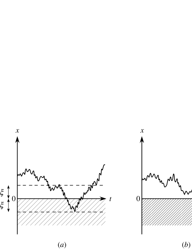
Figure 1: (a) An illustration of a path of surviving Brownian particle in one-dimension with a killing term $-V(x)$ given by (1.2). The parameter $\xi$ is the characteristic length of the interaction to kill a particle acting from the origin. It also indicates the penetration length of a particle into the negative region. (b) An illustration of a path of surviving Brownian particle in the absorbing Brownian motion with an absorbing wall at the origin. It is regarded as the limit $\xi\to 0$ of the system shown in (a).

Let $Q(t,y|x)$ be the transition probability density of this killing Brownian motion from a position $x\in\mathbb{R}$ to a position $y\in\mathbb{R}$ during time $t>0$. It will be obtained by taking an average of (1.3) over all realizations of Brownian path under the conditions $B(0)=y,B(t)=x$. (Note that the time ordering is reversed, since the equation of $Q$ given by (1.5) below is the backward Kolmogorov equation.) That is,

$$Q(t,y|x)={\bf E}\left[\exp\left\{-\int_{0}^{t}V(B(s))ds\right\}{\bf 1}(B(0)=y,B(t)=x)\right],$$ (1.4)

where ${\bf E}[\ \cdot\ ]$ denotes an expectation with respect to Brownian motion, and ${\bf 1}(\omega)$ is the indicator function of a condition $\omega$; ${\bf 1}(\omega)=1$ if $\omega$ is satisfied, and ${\bf 1}(\omega)=0$ otherwise. It is the Feynman-Kac formula (see, e.g., [15]) for the unique solution of the diffusion equation

$$\frac{\partial}{\partial t}Q(t,y|x)=\left(\frac{1}{2}\frac{\partial^{2}}{\partial x^{2}}-V(x)\right)Q(t,y|x)$$ (1.5)

under the initial condition $Q(0,y|x)=\delta(x-y)$.

Let $I_{\nu}(z),z,\nu\in\mathbb{C}$ be the modified Bessel function of the first kind

$$I_{\nu}(z)=\sum_{k=0}^{\infty}\frac{(z/2)^{\nu+2k}}{\Gamma(k+1)\Gamma(k+\nu+1)},\quad|z|<\infty,\quad|{\rm arg}\,z|<\pi,$$ (1.6)

and $K_{\nu}(z),z\in\mathbb{C}$ be Macdonald’s function [37, 25] defined by

$$K_{\nu}(z)=\frac{\pi}{2}\frac{I_{-\nu}(z)-I_{\nu}(z)}{\sin(\nu\pi)},\quad|{\rm arg}\,z|<\pi,\quad\mbox{for}\quad\nu\not=0,\pm 1,\pm 2,\dots,$$ (1.7)

and for integers $\nu=n$,

$$K_{n}(z)=\lim_{\nu\to n}K_{\nu}(z),\quad n=0,\pm 1,\pm 2,\dots,$$ (1.8)

which are both analytic functions of $z$ for all $z$ in the complex plane $\mathbb{C}$ cut along the negative real axis, and entire functions of $\nu$. We see that $I_{\nu}(z)$ and $K_{\nu}(z)$ are linearly independent solutions of the differential equation

$$\frac{d^{2}w}{dz^{2}}+\frac{1}{z}\frac{dw}{dz}-\left(1+\frac{\nu^{2}}{z^{2}}\right)w=0.$$

For $x>0$ and $\nu\geq 0$, $I_{\nu}(x)$ is a positive function which increases monotonically as $x\to\infty$, while $K_{\nu}(x)$ is a positive function which decreases monotonically as $x\to\infty$. Then an integral representation of $Q(t,y|x)$ is given by [26, 27, 28, 17]

$$Q(t,y|x)=\frac{1}{\pi}\int_{-\infty}^{\infty}e^{-k^{2}t/2}K_{i\xi k}(e^{-x/\xi})K_{-i\xi k}(e^{-y/\xi})|\Gamma(i\xi k)|^{-2}dk,$$ (1.9)

where $i=\sqrt{-1}$ and $\Gamma(z)$ is the gamma function.

For each initial position $x\in\mathbb{R}$, the survival probability of this killing Brownian motion at time $T\geq 0$ is obtained by integrating $Q(T,y|x)$ over $y\in\mathbb{R}$,

$${\cal N}(T,x)=\int_{-\infty}^{\infty}Q(T,y|x)dy,\quad x\in\mathbb{R},\quad T\geq 0.$$ (1.10)

If we condition the process to survive up to time $T>0$, the transition probability density from the state $(s,x)$ to $(t,y)$ of the killing Brownian motion is given by

$$P^{T}(s,x;t,y)=\frac{{\cal N}(T-t,y)}{{\cal N}(T-s,x)}Q(t-s,y|x),\quad x,y\in\mathbb{R},\quad 0\leq s\leq t\leq T.$$ (1.11)

If we use the integral representations of $K_{\nu}(z)$ [37, 25],

$$K_{\nu}(z)=\frac{2^{\nu}\Gamma(\nu+1/2)}{z^{\nu}\sqrt{\pi}}\int_{0}^{\infty}\frac{\cos(zu)}{(1+u^{2})^{\nu+1/2}}du,$$ (1.12)

and

$$K_{\nu}(z)=\frac{1}{2}\int_{0}^{\infty}s^{\nu-1}\exp\left\{-\frac{z}{2}\left(s+\frac{1}{s}\right)\right\}ds,$$ (1.13)

we can evaluate the long-term asymptotics of the survival probability for $|x|<\infty$,

$${\cal N}(T,x)=CT^{-1/2}K_{0}(e^{-x/\xi})\times\left\{1+{\cal O}\left(\frac{x}{\sqrt{T}}\right)\right\}\quad\mbox{in}\quad\frac{x}{\sqrt{T}}\to 0$$ (1.14)

with $C=3\xi\sqrt{2/\pi}$ as shown in Appendix A. Then we can take the limit $T\to\infty$ of (1.11) as

$$P(t,y|x) \equiv \lim_{T\to\infty}P^{T}(0,x;t,y)$$ (1.15)

$$= \frac{K_{0}(e^{-y/\xi})}{K_{0}(e^{-x/\xi})}Q(t,y|x),\quad x,y\in\mathbb{R},\quad 0\leq t<\infty.$$

This is the transition probability density of the killing Brownian motion conditioned to survive forever. We should note that this conditional Brownian motion is the diffusion process with infinitesimal generator

$${\cal L}_{\rm MY}=\frac{1}{2}\frac{d^{2}}{dx^{2}}+\frac{d}{dx}\Big{\{}\log K_{0}(e^{-x/\xi})\Big{\}}\frac{d}{dx}.$$ (1.16)

Matsumoto and Yor [26, 27] have studied the exponential functionals of Brownian motion

$$Z_{\rm MY}(t)=\xi\log\left\{\frac{1}{\xi^{2}}\int_{0}^{t}e^{2B(s)/\xi}ds\right\}-B(t),\quad t\geq 0,$$ (1.17)

which is the diffusion process whose infinitesimal generator is (1.16). We can say that the Matsumoto-Yor process (1.17) is realized as the present killing Brownian motion conditioned to survive forever [17].

Now we consider the limit $\xi\to 0$ of the formulas obtained above. Since $I_{\nu}(z)$ is defined as the series expansion (1.6), we can see $I_{i\xi k}(e^{-x/\xi})\simeq(e^{-x/\xi}/2)^{i\xi k}/\Gamma(i\xi k+1)\simeq e^{-ikx}$ in $\xi\to 0$ for $x>0$. Then (1.7) gives $K_{i\xi k}(e^{-x/\xi})\simeq\sin(kx)/(\xi k){\bf 1}(x>0)$ in $\xi\to 0$. Therefore the integral of (1.9) can be performed in the limit and we have

$$q(t,y|x)\equiv\lim_{\xi\to 0}Q(t,y|x)$$

$$\qquad=\frac{1}{\sqrt{2\pi t}}\Big{\{}e^{-(x-y)^{2}/2t}-e^{-(x+y)^{2}/2t}\Big{\}}\,{\bf 1}(x>0,y\geq 0).$$ (1.18)

It is the transition probability density of the absorbing Brownian motion with an absorbing wall at the origin, which is easily obtained by applying the reflection principle of Brownian motion [15]. Applying the result (A.2) shown in Appendix A, we see that

$$\lim_{\xi\to 0}\xi K_{0}(e^{-x/\xi})=x\,{\bf 1}(x>0),$$ (1.19)

and then (1.15) gives in this limit

$$p(t,y|x) \equiv \lim_{\xi\to 0}P(t,y|x)$$ (1.20)

$$= \frac{y}{x}q(t,y|x),\quad x>0,y\geq 0,\quad t\geq 0,$$

which is a harmonic transform ($h$-transform) of (1.18) and is identified with the transition probability density of the three-dimensional Bessel process, BES(3) (see, for instance, [20]). As a matter of fact [26, 27], (1.17) gives $\lim_{\xi\to 0}Z_{\rm MY}(t)=2\sup_{0\leq s\leq t}B(s)-B(t),t\geq 0$, which is indeed distributed as BES(3) (Pitman’s $2M-X$ theorem [30]).

In the present paper, we consider an $N$-particle system of one-dimensional Brownian motions with $N\geq 2$, $\mbox{\boldmath$B$}(t)=(B_{1}(t),\dots,B_{N}(t)),t\geq 0$, with a positive parameter $\xi>0$, such that the probability that all $N$ particles survive up to time $t$, $P_{N}(t)$, decays following the equation

$$\frac{dP_{N}(t)}{dt}=-V_{N}(\mbox{\boldmath$B$}(t))P_{N}(t),\quad t\geq 0$$ (1.21)

with a decay rate function

$$V_{N}(\mbox{\boldmath$x$})=\frac{1}{\xi^{2}}\sum_{j=1}^{N-1}e^{-(x_{j+1}-x_{j})/\xi},\quad\mbox{\boldmath$x$}\in\mathbb{R}^{N}.$$ (1.22)

We study an integral representation of the transition probability density $Q_{N}(t,\mbox{\boldmath$y$}|\mbox{\boldmath$x$}),\mbox{\boldmath$x$},\mbox{\boldmath$y$}\in\mathbb{R}^{N},t\geq 0$, which is a multivariate extension of (1.9). The extensions of the formulas (1.14) and (1.15) are shown. We prove that the $N$-particle system of the mutually killing Brownian motions following (1.21) and (1.22) conditioned that all $N$ particles survive forever is equivalent to a special case (without drift, $\mbox{\boldmath$\nu$}=0$) of the O’Connell process [28, 17].

In the context of quantum mechanics, the decay rate functions of survival probability (1.2) and (1.22) in the killing Brownian motions are considered to giving potential energy of the systems. They are called the Yukawa potential and the Toda-lattice potential [36], respectively. The multivariate extensions of Macdonald’s function (1.7) with (1.8) are the Whittaker functions (see [1, 28, 4, 2, 29] and references therein), which have been extensively studied in mathematical physics as eigenfunctions of the quantum Toda lattice [24, 32, 31, 9, 21, 22, 23, 14, 7, 8]. See also [10].

In Sect.2, as preliminaries, useful integral representations of the Whittaker functions are given for the $GL(N,\mathbb{R})$-quantum Toda lattice. The transition probability density of the system of mutually killing Brownian motions is given, in the case that killing of particles does not occur during an observing time period, as an integral of a product of the Whittaker functions over the Sklyanin measure. Then the main results are given. We also demonstrate that when the characteristic length $\xi$ of the interaction killing other particles goes to zero, the O’Connell process is reduced to the noncolliding Brownian motion, which is known to be equivalent to the Dyson model [11, 20] for the eigenvalue process of Hermitian matrix-valued diffusion process (i.e. Dyson’s Brownian motion model with the parameter $\beta=2$ [5]). The proofs of Lemmas and Proposition are given in Sect.3. Appendix is given for proving (1.14) and (1.19) used above.

2 Preliminaries and Main Results

2.1 Quantum Toda lattice and Whittaker functions

In this subsection we set $\xi=1$ in Eq.(1.22) and consider $V_{N}(\mbox{\boldmath$x$})$ as a potential energy of a quantum $N$-particle system in one dimension. Then we have the Hamiltonian of the $GL(N,\mathbb{R})$-quantum Toda lattice

$${\cal H}_{N}=-\frac{1}{2}\sum_{j=1}^{N}\frac{\partial^{2}}{\partial x_{j}^{2}}+\sum_{j=1}^{N-1}e^{-(x_{j+1}-x_{j})}$$ (2.1)

for $N\in\{2,3,\dots\}$. (In this paper, we set the mass of particle $m=1$ and $\hbar=1$ for simplicity of notation.) The generalized eigenvalue problem

$${\cal H}_{N}\Psi_{\lambda}(\mbox{\boldmath$x$})=\lambda\Psi_{\lambda}(\mbox{\boldmath$x$}),\quad\mbox{\boldmath$x$}\in\mathbb{R}^{N},$$ (2.2)

is solved by setting

$$\lambda=-\frac{1}{2}\sum_{j=1}^{N}\nu_{j}^{2}=-\frac{1}{2}|\mbox{\boldmath$\nu$}|^{2},\quad\mbox{\boldmath$\nu$}=(\nu_{1},\dots,\nu_{N})\in\mathbb{C}^{N}$$ (2.3)

with the eigenfunction $\Psi_{\lambda}(\mbox{\boldmath$x$})=\psi_{\mbox{\boldmath$\nu$}}^{(N)}(\mbox{\boldmath$x$})$, where $\psi_{\mbox{\boldmath$\nu$}}^{(N)}(\mbox{\boldmath$x$})$ is the $GL(N,\mathbb{R})$-Whittaker function [24, 32, 31, 21] (the class-one $\mathfrak{gl}_{N}$-Whittaker function [8, 1, 28, 4, 2]). When $N=2$, it is expressed by using Macdonald’s function (1.7) as

$$\psi_{(\nu_{1},\nu_{2})}^{(2)}(x_{1},x_{2})=2e^{(\nu_{1}+\nu_{2})(x_{1}+x_{2})/2}K_{\nu_{2}-\nu_{1}}(2e^{-(x_{2}-x_{1})/2}).$$

In this sense, the Whittaker functions $\{\psi^{(N)}_{\mbox{\boldmath$\nu$}}(\mbox{\boldmath$x$})\}_{N\geq 2}$ are regarded as multivariate extensions of Macdonald’s function.

Corresponding to the two kinds of integral representations (1.12) and (1.13) for $K_{\nu}(z)$, two integral representations are known for the Whittaker function $\psi_{\mbox{\boldmath$\nu$}}^{(N)}(\mbox{\boldmath$x$}),\mbox{\boldmath$\nu$}\in\mathbb{C}^{N}$. The integral expression corresponding to (1.12) is the classical one originally given by Jacquet [13] and was rewritten as the following form by Stade [33]. (Here we use the notation given by [21].) Let $Z$ denote an upper triangular $N\times N$ matrix with unit diagonal; $\mbox{\boldmath$Z$}=(Z_{j,k})_{1\leq j,k\leq N}$,

$$Z_{j,k}=\left\{\begin{array}[]{ll}z_{j,k},&\quad 1\leq j<k\leq N,\cr 1,&\quad 1\leq j=k\leq N,\cr 0,&\quad 1\leq k<j\leq N.\end{array}\right.$$ (2.4)

We write the integral of a function $f$ of $Z$ over all real $Z$ as

$$\int_{\mathbb{R}^{N(N-1)/2}}f(\mbox{\boldmath$Z$})d\mbox{\boldmath$Z$}\equiv\prod_{k=1}^{N}\prod_{j=1}^{k-1}\int_{-\infty}^{\infty}dz_{j,k}f(\mbox{\boldmath$Z$}).$$

The transpose of $Z$ is denoted by ${}^{t}\!\mbox{\boldmath$Z$}$ and the principal minor of size $j$ of matrix $\mbox{\boldmath$Z$}\,{{}^{t}\!\mbox{\boldmath$Z$}}$ is written as $\Delta_{j}(\mbox{\boldmath$Z$}\,{{}^{t}\!\mbox{\boldmath$Z$}}),1\leq j\leq N$. For $\mbox{\boldmath$x$}=(x_{1},\dots,x_{N})\in\mathbb{R}^{N},\mbox{\boldmath$\nu$}=(\nu_{1},\dots,\nu_{N})\in\mathbb{C}^{N}$,

$$\psi_{\mbox{\boldmath$\nu$}}^{(N)}(\mbox{\boldmath$x$})=\exp(\mbox{\boldmath$\nu$}\cdot\mbox{\boldmath$x$})\prod_{1\leq j<k\leq N}\frac{\Gamma(\nu_{k}-\nu_{j}+1/2)}{\sqrt{\pi}}$$

$$\qquad\times\int_{\mathbb{R}^{N(N-1)/2}}\prod_{j=1}^{N-1}\Bigg{[}\Delta_{j}(\mbox{\boldmath$Z$}\,{{}^{t}\!\mbox{\boldmath$Z$}})^{\nu_{j}-\nu_{j+1}-1/2}\exp\Big{\{}2iz_{j,j+1}e^{-(x_{j+1}-x_{j})/2}\Big{\}}\Bigg{]}d\mbox{\boldmath$Z$}.$$ (2.5)

Another integral representation, which corresponds to (1.13), was given by Givental [9]. See also [23, 7]. Let $T$ denote a lower triangular array with size $N$, $\mbox{\boldmath$T$}=(T_{j,k},1\leq k\leq j\leq N)$. For a given $\mbox{\boldmath$x$}\in\mathbb{R}^{N}$, let $\Gamma_{N}(\mbox{\boldmath$x$})$ be the space of all real triangular arrays $T$ with size $N$ conditioned

$$T_{N,k}=x_{k},\quad 1\leq k\leq N.$$ (2.6)

We write the integral of a function $f$ of $T$ over $\Gamma_{N}(\mbox{\boldmath$x$})$ as

$$\int_{\Gamma_{N}(\mbox{\boldmath$x$})}f(\mbox{\boldmath$T$})d\mbox{\boldmath$T$}\equiv\prod_{j=1}^{N}\prod_{k=1}^{j}\int_{-\infty}^{\infty}dT_{j,k}\,f(\mbox{\boldmath$T$})\prod_{\ell=1}^{N}\delta(T_{N,\ell}-x_{\ell}).$$

Then

$$\psi_{\mbox{\boldmath$\nu$}}^{(N)}(\mbox{\boldmath$x$}) = \int_{\Gamma_{N}(\mbox{\boldmath$x$})}\exp\left[\sum_{j=1}^{N}\nu_{j}\left(\sum_{k=1}^{j}T_{j,k}-\sum_{k=1}^{j-1}T_{j-1,k}\right)\right.$$ (2.7)

$$\quad\left.-\sum_{j=1}^{N-1}\sum_{k=1}^{j}\Big{\{}e^{-(T_{j,k}-T_{j+1,k})}+e^{-(T_{j+1,k+1}-T_{j,k})}\Big{\}}\right]d\mbox{\boldmath$T$}.$$

Remark 1.   There is the ‘third’ kind of integral representation of the Whittaker function,

$$\psi_{\mbox{\boldmath$\nu$}}^{(N)}(\mbox{\boldmath$x$}) = \int_{{\cal S}}\prod_{j=1}^{N-1}\frac{\prod_{k=1}^{j}\prod_{\ell=1}^{j+1}\Gamma(\gamma_{j+1,\ell}-\gamma_{j,k})}{(2\pi)^{j}j!\prod_{1\leq k<\ell\leq j}|\Gamma(\gamma_{j,\ell}-\gamma_{j,k})|^{2}}$$ (2.8)

$$\quad\times\exp\left\{i\sum_{j=1}^{N}\sum_{k=1}^{j}(\gamma_{j,k}-\gamma_{j-1,k})x_{j}\right\}\prod_{j=1}^{N-1}\prod_{k=1}^{j}d\gamma_{j,k},$$

where $(\gamma_{N,1},\dots,\gamma_{N,N})\equiv(\nu_{1},\dots,\nu_{N})$, $\gamma_{j,k}=0$ for $k>j$, and the domain of integration ${\cal S}$ is defined by the conditions $\min_{k}\{{\rm Im}\gamma_{j,k}\}>\max_{k}\{{\rm Im}\gamma_{j+1,k}\}$ for all $j=1,2,\dots,N-1$. This is called the Mellin-Barnes integral representation, since it can be regarded as the multivariate extension of the Mellin-Barnes representation of Macdonald’s function [37]

$$K_{\nu}(z)=\frac{1}{8\pi i}\int_{{\cal C}}\Gamma\left(\frac{s+\nu}{2}\right)\Gamma\left(\frac{s-\nu}{2}\right)\left(\frac{z}{2}\right)^{-2}ds,$$

where the path of integration ${\cal C}$ being a vertical line to the right of any poles of the integrand. The derivation of the Mellin-Barnes integral representation (2.8) from the classical one (2.5) is shown in [34, 12] (see also [22, 23]). The equivalence between the Givental integral representation (2.7) and the Mellin-Barnes integral representation (2.8) is fully discussed in [8].

2.2 Transition probability density of the mutually killing Brownian motions

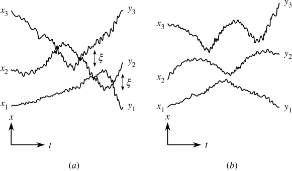
Figure 2: (1) An illustration of three paths of surviving Brownian particles in the mutually killing Brownian motions. The effect of killing is not negligible when the distance between the nearest neighbor pair of particles is less than $\xi$; $B_{j+1}(t)-B_{j}(t)<\xi$. The ordering of particle positions can be changed, but the risk of pair annihilation becomes large exponentially, when $B_{j}(t)-B_{j+1}(t)>\xi$. (b) In the limit $\xi\to 0$, the present system converges to the vicious Brownian motion, in which the process survives if and only if paths are not intersecting.

For $N\in\{2,3,\dots\}$, we consider the $N$-particle system of mutually killing Brownian motions, in which the probability that all $N$ particles survive decays in time following (1.21) with (1.22) depending on realization of paths. For $\mbox{\boldmath$x$},\mbox{\boldmath$y$}\in\mathbb{R}^{N},t\geq 0$, the transition probability density from the state $x$ to $y$ during time interval $t$ is then given by

$$Q_{N}(t,\mbox{\boldmath$y$}|\mbox{\boldmath$x$})={\bf E}\left[\exp\left\{-\int_{0}^{t}V_{N}(\mbox{\boldmath$B$}(s))ds\right\}{\bf 1}(\mbox{\boldmath$B$}(0)=\mbox{\boldmath$y$},\mbox{\boldmath$B$}(t)=\mbox{\boldmath$x$})\right]$$

$$\quad={\bf E}\left[\exp\left\{-\frac{1}{\xi^{2}}\sum_{j=1}^{N-1}\int_{0}^{t}e^{-(B_{j+1}(s)-B_{j}(s))/\xi}ds\right\}{\bf 1}(\mbox{\boldmath$B$}(0)=\mbox{\boldmath$y$},\mbox{\boldmath$B$}(t)=\mbox{\boldmath$x$})\right].$$ (2.9)

It is the Feynman-Kac formula for the solution of the diffusion equation (the backward Kolmogorov equation)

$$\frac{\partial u(t,\mbox{\boldmath$x$})}{\partial t}=\frac{1}{2}\Delta u(t,\mbox{\boldmath$x$})-V_{N}(\mbox{\boldmath$x$})u(t,\mbox{\boldmath$x$})$$ (2.10)

with $\Delta=\sum_{j=1}^{N}\partial^{2}/\partial x_{j}^{2}$ under the initial condition

$$u(0,\mbox{\boldmath$x$})=\delta(\mbox{\boldmath$x$}-\mbox{\boldmath$y$})\equiv\prod_{j=1}^{N}\delta(x_{j}-y_{j}).$$ (2.11)

Remark 2. If we regard (2.10) as a diffusion equation describing an $N$-dimensional Brownian motion in $\mathbb{R}^{N}$ with a killing term $-V_{N}(\mbox{\boldmath$x$})$, (2.9) gives a transition probability density for a particle assumed to be at a position $\mbox{\boldmath$x$}\in\mathbb{R}^{N}$ such that it survives during time $t$ and it arrives at a position $\mbox{\boldmath$y$}\in\mathbb{R}^{N}$ after the time duration $t$ (the Feynman-Kac formula, see, for instance, [15]). In the present paper, on the other hand, we would like to consider an $N$-particle system of one-dimensional Brownian motions, such that the $j$-th and $(j+1)$-th particles will be pair annihilated with high probability if $B_{j+1}(t)-B_{j}(t)<\xi,1\leq j\leq N-1$, and then the probability that all $N$ particles survive avoiding from any mutual killing decays in time following (1.21) with (1.22). In order to discuss processes, in which mutual killing of particles actually occurs and total number of particles decreases in time, we have to specify the stochastic rule to determine which pair of particles is annihilated, when the survival probability conditional on a path, $\exp\{-\int_{0}^{t}V_{N}(\mbox{\boldmath$B$}(s))ds\}$, becomes small. Here we are interested in, however, the situation that mutual killing of particles does not occur at all and all $N$ particles survive, following the notion of vicious walker models [6, 18, 3, 17]. The Feynman-Kac formula (2.9) gives the transition probability density between $N$-particle configurations $\mbox{\boldmath$x$},\mbox{\boldmath$y$}\in\mathbb{R}^{N}$. Figure 2(a) illustrates three paths of surviving particles, in which change of ordering of particle positions occurs within the spatial scale $\simeq\xi$.

By the fact that the Whittaker function $\psi_{\mbox{\boldmath$k$}}^{(N)}(\mbox{\boldmath$x$})$ solves (2.2) with (2.3), we can see that

$$\exp\left(-\frac{t}{2}|\mbox{\boldmath$k$}|^{2}\right)\psi_{i\xi\mbox{\boldmath$k$}}^{(N)}(\mbox{\boldmath$x$}/\xi),\quad|\mbox{\boldmath$k$}|^{2}\equiv\sum_{j=1}^{N}k_{j}^{2},\quad\mbox{\boldmath$k$}\in\mathbb{R}^{N},$$ (2.12)

solves the diffusion equation (2.10).

The density function of the Sklyanin measure [32] is defined by

$$s_{N}(\mbox{\boldmath$k$})=\frac{1}{(2\pi)^{N}N!}\prod_{1\leq j<\ell\leq N}|\Gamma(i(k_{\ell}-k_{j}))|^{-2}$$ (2.13)

for $\mbox{\boldmath$k$}\in\mathbb{C}^{N}$. By Euler’s reflection formula $\Gamma(z)\Gamma(1-z)=\pi/\sin(\pi z)$, if $\mbox{\boldmath$k$}\in\mathbb{R}^{N}$,

$$\prod_{1\leq j<\ell\leq N}|\Gamma(i(k_{\ell}-k_{j}))|^{-2}=\prod_{1\leq j<\ell\leq N}\left\{(k_{\ell}-k_{j})\frac{\sinh\pi(k_{\ell}-k_{j})}{\pi}\right\}.$$

Since the Whittaker functions satisfy the completeness relation with respect to the Sklyanin measure $s_{N}(\mbox{\boldmath$k$})d\mbox{\boldmath$k$}\equiv s_{N}(\mbox{\boldmath$k$})\prod_{j=1}^{N}dk_{j}$ [31, 21, 23, 8],

$$\int_{\mathbb{R}^{N}}\psi^{(N)}_{i\mbox{\boldmath$k$}}(\mbox{\boldmath$x$})\psi^{(N)}_{-i\mbox{\boldmath$k$}}(\mbox{\boldmath$y$})s_{N}(\mbox{\boldmath$k$})d\mbox{\boldmath$k$}=\delta(\mbox{\boldmath$x$}-\mbox{\boldmath$y$}),\quad\mbox{\boldmath$x$},\mbox{\boldmath$y$}\in\mathbb{R}^{N},$$ (2.14)

the integral of the solution (2.12) multiplied by $\psi^{(N)}_{-i\xi\mbox{\boldmath$k$}}(\mbox{\boldmath$y$}/\xi)$ on this measure,

$$Q_{N}(t,\mbox{\boldmath$y$}|\mbox{\boldmath$x$})=\int_{\mathbb{R}^{N}}e^{-t|\mbox{\boldmath$k$}|^{2}/2}\psi_{i\xi\mbox{\boldmath$k$}}^{(N)}(\mbox{\boldmath$x$}/\xi)\psi_{-i\xi\mbox{\boldmath$k$}}^{(N)}(\mbox{\boldmath$y$}/\xi)s_{N}(\xi\mbox{\boldmath$k$})d\mbox{\boldmath$k$}$$ (2.15)

satisfies the initial condition (2.11). That is, (2.15) is an integral representation of the transition probability density (2.9). It should be noted that the orthogonality relation [21, 8]

$$\int_{\mathbb{R}^{N}}\psi_{-i\mbox{\boldmath$k$}}^{(N)}(\mbox{\boldmath$x$})\psi_{i\mbox{\boldmath$k$}^{\prime}}^{(N)}(\mbox{\boldmath$x$})d\mbox{\boldmath$x$}=\frac{1}{s_{N}(\mbox{\boldmath$k$})N!}\sum_{\sigma\in{\cal S}_{N}}\delta(\mbox{\boldmath$k$}-\sigma(\mbox{\boldmath$k$}^{\prime})),\quad\mbox{\boldmath$k$},\mbox{\boldmath$k$}^{\prime}\in\mathbb{R}^{N},$$ (2.16)

is established, where ${\cal S}_{N}$ is a set of all permutation of $N$ indices and $\sigma(\mbox{\boldmath$k$}^{\prime})\equiv(k^{\prime}_{\sigma(1)},\dots,k^{\prime}_{\sigma(N)})$. It guarantees the Chapman-Kolmogorov equation for the transition probability density

$$\int_{\mathbb{R}^{N}}Q_{N}(t_{2},\mbox{\boldmath$z$}|\mbox{\boldmath$y$})Q_{N}(t_{1},\mbox{\boldmath$y$}|\mbox{\boldmath$x$})d\mbox{\boldmath$y$}=Q_{N}(t_{1}+t_{2},\mbox{\boldmath$z$}|\mbox{\boldmath$x$}),\quad\mbox{\boldmath$x$},\mbox{\boldmath$z$}\in\mathbb{R}^{N}$$ (2.17)

for $0\leq t_{1},t_{2}<\infty$, which should hold, since the present process is Markovian.

Remark 3.   The completeness relation (2.14) of the Whittaker functions is a multivariate extension of the relation for Macdonald’s functions,

$$\frac{1}{\pi^{2}}\int_{\mathbb{R}}K_{ik}(e^{-x})K_{-ik}(e^{-y})k\sinh(\pi k)dk=\delta(x-y),\quad x,y\in\mathbb{R},$$ (2.18)

which will define the Kontorovich-Lebedev transform [25]. We can use (2.18) to confirm that (1.9) satisfies the initial condition $Q(0,y|x)=\delta(x-y)$.

2.3 Asymptotics of transition probability density and survival probability

By using the integral representation (2.5), we can prove the following asymptotics of the transition probability density.

Lemma 2.1

For $\mbox{\boldmath$x$},\mbox{\boldmath$y$}\in\mathbb{R}^{N},|\mbox{\boldmath$x$}|<\infty,t>0$, as $|\mbox{\boldmath$x$}|/\sqrt{t}\to 0$,

$$Q_{N}(t,\mbox{\boldmath$y$}|\mbox{\boldmath$x$})=\xi^{N(N-1)}\frac{1}{(2\pi)^{N}N!}\left(\frac{2}{t}\right)^{N^{2}/2}\psi_{0}^{(N)}(\mbox{\boldmath$x$}/\xi)\psi_{0}^{(N)}(\mbox{\boldmath$y$}/\xi)e^{-|\mbox{\boldmath$y$}|^{2}/2t}$$

$$\quad\times\int_{\mathbb{R}^{N}}e^{-|\mbox{\boldmath$\mu$}|^{2}}\prod_{1\leq j<k\leq N}\left[(\mu_{k}-\mu_{j})^{2}+\frac{1}{2t}(y_{k}-y_{j})^{2}\right]d\mbox{\boldmath$\mu$}\times\left\{1+{\cal O}\left(\frac{|\mbox{\boldmath$x$}|}{\sqrt{t}}\right)\right\}.$$ (2.19)

On the other hand, by using Givental’s integral representation (2.7), we have the following [28]. Let $\mathbb{W}_{N}$ be the Weyl chamber of type A_N-1,

$$\mathbb{W}_{N}=\{\mbox{\boldmath$x$}=(x_{1},x_{2},\dots,x_{N})\in\mathbb{R}^{N}:x_{1}<x_{2}<\cdots<x_{N}\}$$

and set

$$h_{N}(\mbox{\boldmath$x$})=\prod_{1\leq j<k\leq N}(x_{k}-x_{j}).$$ (2.20)

Lemma 2.2

For $\mbox{\boldmath$x$}\in\mathbb{R}^{N}$,

$$\lim_{\beta\to\infty}\beta^{-N(N-1)/2}\psi_{0}^{(N)}(\beta\mbox{\boldmath$x$})=\frac{h_{N}(\mbox{\boldmath$x$})}{\prod_{j=1}^{N-1}j!}{\bf 1}(\mbox{\boldmath$x$}\in\mathbb{W}_{N}).$$ (2.21)

The probability that all $N$ particles survive up to time $t$ in this system of the mutually killing Brownian motions is given by

$${\cal N}_{N}(t,\mbox{\boldmath$x$})=\int_{\mathbb{R}^{N}}Q_{N}(t,\mbox{\boldmath$y$}|\mbox{\boldmath$x$})d\mbox{\boldmath$y$}$$ (2.22)

for each initial state $\mbox{\boldmath$x$}\in\mathbb{R}^{N}$. We call it simply the survival probability in this paper. The following long-term asymptotics of the survival probability is obtained.

Proposition 2.3

Let

$$C_{N}=\xi^{N(N-1)/2}\frac{2^{3N(N-1)/4}}{\pi^{N}\prod_{j=1}^{N-1}j!}A_{N}$$ (2.23)

with

$$A_{N}=\int_{\mathbb{W}_{N}}d\mbox{\boldmath$\eta$}\int_{\mathbb{W}_{N}}d\mbox{\boldmath$\mu$}\,e^{-(|\mbox{\boldmath$\eta$}|^{2}+|\mbox{\boldmath$\mu$}|^{2})}\prod_{1\leq j<k\leq N}\Big{[}(\eta_{k}-\eta_{j})\{(\mu_{k}-\mu_{j})^{2}+(\eta_{k}-\eta_{j})^{2}\}\Big{]}.$$ (2.24)

Then for $\mbox{\boldmath$x$}\in\mathbb{R}^{N}$,

$$\lim_{t\to\infty}t^{N(N-1)/4}{\cal N}_{N}(t,\mbox{\boldmath$x$})=C_{N}\psi_{0}^{(N)}(\mbox{\boldmath$x$}/\xi).$$ (2.25)

2.4 O’Connell process as a system of mutually killing Brownian motions conditioned that all particles survive forever

Let $0\leq T<\infty$ and we consider the $N$-particle system of the mutually killing Brownian motions conditioned that all particles survive up to time $T$. For $0\leq s\leq t\leq T$, the transition probability density from the state $(s,\mbox{\boldmath$x$})$ to $(t,\mbox{\boldmath$y$}),\mbox{\boldmath$x$},\mbox{\boldmath$y$}\in\mathbb{R}^{N}$ of this conditional process is given by

$$P_{N}^{T}(s,\mbox{\boldmath$x$};t,\mbox{\boldmath$y$})=\frac{{\cal N}_{N}(T-t,\mbox{\boldmath$y$})}{{\cal N}_{N}(T-s,\mbox{\boldmath$x$})}Q_{N}(t-s,\mbox{\boldmath$y$}|\mbox{\boldmath$x$}),\quad 0\leq s\leq t\leq T.$$ (2.26)

The fact that (2.26) depends not only $t-s$ but also $T-t$ and $T-t$ implies that this conditional process is inhomogeneous in time.

Proposition 2.3 enables us to take the limit $T\to\infty$ of (2.26). As a result we obtain the temporally homogeneous process with the transition probability density

$$P_{N}(t,\mbox{\boldmath$y$}|\mbox{\boldmath$x$}) \equiv \lim_{T\to\infty}P_{N}^{T}(0,\mbox{\boldmath$x$};t,\mbox{\boldmath$y$})$$ (2.27)

$$= \frac{\psi_{0}^{(N)}(\mbox{\boldmath$y$}/\xi)}{\psi_{0}^{(N)}(\mbox{\boldmath$x$}/\xi)}Q_{N}(t,\mbox{\boldmath$y$}|\mbox{\boldmath$x$}),\quad\mbox{\boldmath$x$},\mbox{\boldmath$y$}\in\mathbb{R}^{N},t\geq 0.$$

It is easy to confirm the following [17].

Proposition 2.4

The transition probability density (2.27) of the $N$-particle system of the mutually killing Brownian motions conditioned that all particles survive forever solves the following diffusion equation,

$$\frac{\partial}{\partial t}u(t,\mbox{\boldmath$x$})=\frac{1}{2}\Delta u(t,\mbox{\boldmath$x$})+\nabla\log\psi_{0}^{(N)}(\mbox{\boldmath$x$}/\xi)\cdot\nabla u(t,\mbox{\boldmath$x$})$$

$$=\frac{1}{2}\sum_{j=1}^{N}\frac{\partial^{2}}{\partial x_{j}^{2}}u(t,\mbox{\boldmath$x$})+\sum_{1\leq j\leq N}\frac{\partial\log\psi_{0}^{(N)}(\mbox{\boldmath$x$}/\xi)}{\partial x_{j}}\frac{\partial}{\partial x_{j}}u(t,\mbox{\boldmath$x$}),\quad\mbox{\boldmath$x$}\in\mathbb{R}^{N},t\geq 0,$$ (2.28)

under the initial condition $u(0,\mbox{\boldmath$x$})=\delta(\mbox{\boldmath$x$}-\mbox{\boldmath$y$}),\mbox{\boldmath$y$}\in\mathbb{R}^{N}$.

Recently O’Connell [28] introduced a diffusion process in $\mathbb{R}^{N}$ with the infinitesimal generator of the process

$${\cal L}^{\mbox{\boldmath$\nu$}}_{N} = -(\psi^{(N)}_{\mbox{\boldmath$\nu$}})^{-1}\Big{(}{\cal H}_{N}+|\mbox{\boldmath$\nu$}|^{2}\Big{)}\psi^{(N)}_{\mbox{\boldmath$\nu$}}$$ (2.29)

$$= \frac{1}{2}\Delta+\nabla\log\psi^{(N)}_{\mbox{\boldmath$\nu$}}(\mbox{\boldmath$x$})\cdot\nabla$$

with drift $\mbox{\boldmath$\nu$}\in\mathbb{R}^{N}$. Then we can state the following.

Theorem 2.5

The O’Connell process without drift, $\mbox{\boldmath$\nu$}=0$, is realized as the system of mutually killing Brownian motions conditioned that all particles survive forever.

In an earlier paper [17], we considered the system of mutually killing Brownian motions with drifts $\mbox{\boldmath$\nu$}=(\nu_{1},\dots,\nu_{N})\in\mathbb{R}^{N}$ conditioned that all particles survive forever and took the limit $\mbox{\boldmath$\nu$}\to 0$ to realize the O’Connell process without drift $\mbox{\boldmath$\nu$}=0$. In the present paper we have shown that an introduction of drift $\nu$ is not necessary to deriving (2.27) and concluding Theorem 2.5.

2.5 The $\xi\to 0$ limit

It is known that the functions $\{m^{(N)}(\mbox{\boldmath$x$},\mbox{\boldmath$k$})\}_{\mbox{\boldmath$k$}\in\mathbb{R}^{N}}$ called the fundamental Whittaker functions are defined so that the (class-one) Whittaker functions discussed so far are expressed by the following alternating sum of them [21, 1],

$$\psi^{(N)}_{i\mbox{\boldmath$k$}}(\mbox{\boldmath$x$})=\prod_{1\leq j<\ell\leq N}\frac{\pi}{i\sinh\pi(k_{\ell}-k_{j})}\sum_{\sigma\in{\cal S}_{N}}{\rm sgn}(\sigma)m^{(N)}(\mbox{\boldmath$x$},\sigma(\mbox{\boldmath$k$})),$$ (2.30)

where $\sigma(\mbox{\boldmath$k$})=(k_{\sigma(1)},\dots,k_{\sigma(N)})$ for each permutation $\sigma\in{\cal S}_{N}$. The functions $\{m^{(N)}(\mbox{\boldmath$x$},\mbox{\boldmath$k$})\}_{\mbox{\boldmath$k$}\in\mathbb{R}^{N}}$ are normalized as

$$\lim_{\xi\to 0}m^{(N)}(\mbox{\boldmath$x$}/\xi,\xi\mbox{\boldmath$k$})=e^{i\mbox{\boldmath$k$}\cdot\mbox{\boldmath$x$}}\quad\mbox{for $\mbox{\boldmath$x$}\in\mathbb{W}_{N}$}.$$ (2.31)

Note that (2.30) is a multivariate extension of the definition (1.7) of $K_{\nu}(z)$, which is given by an alternating sum of $I_{\nu}(z)$ and $I_{-\nu}(z)$. Therefore, when $\mbox{\boldmath$x$},\mbox{\boldmath$y$}\in\mathbb{W}_{N}$, we can see that (2.15) with (2.13) gives

$$q_{N}(t,\mbox{\boldmath$y$}|\mbox{\boldmath$x$}) \equiv \lim_{\xi\to 0}Q_{N}(t,\mbox{\boldmath$y$}|\mbox{\boldmath$x$})$$ (2.32)

$$= \frac{1}{(2\pi)^{N}N!}\sum_{\sigma\in{\cal S}_{N}}\sum_{\sigma^{\prime}\in{\cal S}_{N}}{\rm sgn}(\sigma){\rm sgn}(\sigma^{\prime})\int_{\mathbb{R}^{N}}e^{-t|\mbox{\boldmath$k$}|^{2}/2+i(\sigma(\mbox{\boldmath$k$})\cdot\mbox{\boldmath$x$}-\sigma^{\prime}(\mbox{\boldmath$k$})\cdot\mbox{\boldmath$y$})}d\mbox{\boldmath$k$}$$

$$= \frac{1}{(2\pi)^{N}}\sum_{\rho\in{\cal S}_{N}}{\rm sgn}(\rho)\int_{\mathbb{R}^{N}}e^{-t|\mbox{\boldmath$k$}|^{2}/2+i\mbox{\boldmath$k$}\cdot(\mbox{\boldmath$x$}-\rho(\mbox{\boldmath$y$}))}d\mbox{\boldmath$k$}$$

$$= \frac{1}{(2\pi)^{N}}\sum_{\rho\in{\cal S}_{N}}{\rm sgn}(\rho)\left(\frac{2\pi}{t}\right)^{N/2}e^{-|\mbox{\boldmath$x$}-\rho(\mbox{\boldmath$y$})|^{2}/2t}$$

$$= \det_{1\leq j,k\leq N}\left[\frac{1}{\sqrt{2\pi t}}e^{-(x_{j}-y_{k})^{2}/2t}\right].$$

This is the Karlin-McGregor determinant giving a total mass of nonintersecting paths of Brownian motions from $\mbox{\boldmath$x$}\in\mathbb{W}_{N}$ to $\mbox{\boldmath$y$}\in\mathbb{W}_{N}$ during time $t$ [16, 20]. As a matter of fact, when $\mbox{\boldmath$x$},\mbox{\boldmath$y$}\in\mathbb{W}_{N}$, the limit $\xi\to 0$ of (2.9) should give the transition probability density of the $N$-dimensional absorbing Brownian motion in the Weyl chamber $\mathbb{W}_{N}$ (the vicious Brownian motion [17]). See Fig.2(b). Lemma 2.2 implies that, if $\mbox{\boldmath$x$},\mbox{\boldmath$y$}\in\mathbb{W}_{N}$,

$$p_{N}(t,\mbox{\boldmath$y$}|\mbox{\boldmath$x$}) \equiv \lim_{\xi\to 0}P_{N}(t,\mbox{\boldmath$y$}|\mbox{\boldmath$x$})$$ (2.33)

$$= \frac{h_{N}(\mbox{\boldmath$y$})}{h_{N}(\mbox{\boldmath$x$})}q_{N}(t,\mbox{\boldmath$y$}|\mbox{\boldmath$x$}),\quad t\geq 0,$$

which is an $h$-transform of $q_{N}$ by the Vandermonde determinant (2.20). It shows that the limit $\xi\to 0$ of the O’Connell process is identified with the Dyson model (Dyson’s Brownian motion model with $\beta=2$ [5]), which is the $N$-particle system of Brownian motions conditioned never to collide with each other (the noncolliding Brownian motion) [18, 19, 20].

Remark 4.  The survival probability up to time $T<\infty$ of the one-dimensional absorbing Brownian motion with an absorbing wall at the origin is given by

$${\cal N}^{0}(T,x)=\int_{-\infty}^{\infty}q(T,y|x)dy,$$ (2.34)

where the transition probability density $q$ is given by (1.18). The long-term behavior is readily obtained as

$${\cal N}^{0}(T,x)\simeq c^{0}xT^{-\phi},\quad x>0,\quad T\to\infty$$ (2.35)

with $c^{0}=\sqrt{2/\pi},\phi=1/2$. Therefore, the exponent $\phi$ is the same with that found in the asymptotics (1.14) of the survival probability of the killing Brownian motion discussed in Sect.1;

$${\cal N}(T,x)\simeq 3\sqrt{\frac{2}{\pi}}\xi K_{0}(e^{-x/\xi})T^{-\phi},\quad x\in\mathbb{R},\quad T\to\infty.$$ (2.36)

If we take the limit $\xi\to 0$, (1.19) gives

$$\lim_{\xi\to 0}{\cal N}(T,x)\simeq cxT^{-\phi},\quad x>0,\quad T\to\infty$$ (2.37)

with $c=3\sqrt{2/\pi}=3c^{0}$. For $N\geq 2$, Proposition 2.3 implies

$${\cal N}_{N}(T,\mbox{\boldmath$x$})\simeq C_{N}\psi^{(N)}_{0}(\mbox{\boldmath$x$}/\xi)T^{-\phi_{N}},\quad\mbox{\boldmath$x$}\in\mathbb{R}^{N},\quad T\to\infty$$ (2.38)

with $C_{N}$ given by (2.23) and with the survival probability exponent

$$\phi_{N}=\frac{1}{4}N(N-1)$$ (2.39)

for the present $N$-particle system of mutually killing Brownian motion. This exponent is the same as that for the vicious Brownian motion (the absorbing Brownian motion in $\mathbb{W}_{N}$) [6, 18];

$${\cal N}^{0}_{N}(T,\mbox{\boldmath$x$}) \equiv \int_{\mathbb{W}^{N}}q_{N}(T,\mbox{\boldmath$y$}|\mbox{\boldmath$x$})d\mbox{\boldmath$y$}$$ (2.40)

$$\simeq c_{N}^{0}h_{N}(\mbox{\boldmath$x$})T^{-\phi_{N}},\quad\mbox{\boldmath$x$}\in\mathbb{W}_{N},\quad T\to\infty$$

with

$$c_{N}^{0}=\frac{2^{N/2}\prod_{j=1}^{N}\Gamma(j/2)}{\pi^{N/2}\prod_{j=1}^{N-1}j!}.$$ (2.41)

Lemma 2.2 gives then

$$\lim_{\xi\to 0}{\cal N}_{N}(T,\mbox{\boldmath$x$})\simeq c_{N}h_{N}(\mbox{\boldmath$x$})T^{-\phi_{N}},\quad\mbox{\boldmath$x$}\in\mathbb{W}_{N},\quad T\to\infty,$$ (2.42)

where

$$c_{N}=\frac{2^{3N(N-1)/4}}{\pi^{N}\prod_{j=1}^{N-1}(j!)^{2}}A_{N}$$ (2.43)

with (2.24). The above results $c\not=c^{0}$ and $c_{N}\not=c_{N}^{0},N\geq 2$ are consequences of the facts that for the transition probability densities $Q(t,y|x)$ and $Q_{N}(t,\mbox{\boldmath$y$}|\mbox{\boldmath$x$}),N\geq 2$, the long-term limit $T\to\infty$ and the limit $\xi\to 0$ are noncommutable.

3 Proofs of Lemmas and Proposition

3.1 Proof of Lemma 2.1

By the integral representation (2.5), we put $\psi^{(N)}_{i\xi\mbox{\boldmath$k$}}(\mbox{\boldmath$x$}/\xi)=\exp(i\mbox{\boldmath$k$}\cdot\mbox{\boldmath$x$})\widehat{\psi}^{(N)}_{i\xi\mbox{\boldmath$k$}}(\mbox{\boldmath$x$}/\xi)$. Then by changing the integral variables as $\mu_{j}=\sqrt{t/2}k_{j}-i(x_{j}-y_{j})/\sqrt{2t},1\leq j\leq N$, (2.15) with (2.13) is written as

$$Q_{N}(t,\mbox{\boldmath$y$}|\mbox{\boldmath$x$})=\frac{1}{(2\pi)^{N}N!}\left(\frac{2}{t}\right)^{N/2}e^{-|\mbox{\boldmath$x$}-\mbox{\boldmath$y$}|^{2}/2t}$$

$$\quad\times\int_{\mathbb{R}^{N}}e^{-|\mbox{\boldmath$\mu$}|^{2}}\widehat{\psi}^{(N)}_{i\mbox{\boldmath$\alpha$}(\mbox{\boldmath$\mu$})}(\mbox{\boldmath$x$}/\xi)\widehat{\psi}^{(N)}_{-i\mbox{\boldmath$\alpha$}(\mbox{\boldmath$\mu$})}(\mbox{\boldmath$y$}/\xi)\prod_{1\leq j<k\leq N}\Big{|}\Gamma(i(\alpha_{k}(\mu_{k})-\alpha_{j}(\mu_{j})))\Big{|}^{-2}d\mbox{\boldmath$\mu$},$$

where

$$\alpha_{j}(\mu_{j})=\xi\sqrt{\frac{2}{t}}\left\{\mu_{j}+\frac{i}{\sqrt{2t}}(x_{j}-y_{j})\right\},\quad 1\leq j\leq N,$$

and $\mbox{\boldmath$\alpha$}(\mbox{\boldmath$\mu$})=(\alpha_{1}(\mu_{1}),\dots,\alpha_{N}(\mu_{N}))$. For $|\mbox{\boldmath$x$}|<\infty$, in the limit $|\mbox{\boldmath$x$}|/\sqrt{t}\to 0$, $\alpha_{j}(\mu_{j})\simeq\xi\sqrt{2/t}\{\mu_{j}-iy_{j}/\sqrt{2t}\}\to 0,1\leq j\leq N$, and thus $\widehat{\psi}^{(N)}_{i\mbox{\boldmath$\alpha$}(\mbox{\boldmath$\mu$})}(\mbox{\boldmath$x$}/\xi)\to\widehat{\psi}^{(N)}_{0}(\mbox{\boldmath$x$}/\xi)\equiv\psi^{(N)}_{0}(\mbox{\boldmath$x$}/\xi)$. Since $z\Gamma(z)\to 1$ as $z\to 0$,

$$\Big{|}\Gamma(i(\alpha_{k}(\mu_{k})-\alpha_{j}(\mu_{j})))\Big{|}^{-2}\simeq\xi^{2}\frac{2}{t}\left\{(\mu_{k}-\mu_{j})^{2}+\frac{1}{2t}(y_{k}-y_{j})^{2}\right\}$$

in this limit. Then (2.19) is obtained. ∎

3.2 Proof of Lemma 2.2

The following argument is found in Section 6 of O’Connell [28]. For $N\geq 2$, the Gelfand-Tsetlin pattern (complete branching) is defined as [35]

$$\mathbb{GT}_{N} = \Big{\{}(\mbox{\boldmath$x$}^{1},\mbox{\boldmath$x$}^{2},\dots,\mbox{\boldmath$x$}^{N})\in\overline{\mathbb{W}}_{1}\times\overline{\mathbb{W}}_{2}\times\cdots\times\overline{\mathbb{W}}_{N}:$$ (3.1)

$$\qquad\quad x^{j+1}_{k}\leq x^{j}_{k}\leq x^{j+1}_{k+1},1\leq k\leq j\leq N-1\Big{\}},$$

where $\overline{\mathbb{W}}_{j}=\{\mbox{\boldmath$x$}=(x_{1},\dots,x_{j})\in\mathbb{R}^{j}:x_{1}\leq\cdots\leq x_{j}\},1\leq j\leq N$. By the Givental integral representation (2.7),

$$\psi_{0}^{(N)}(\beta\mbox{\boldmath$x$}) = \int_{\Gamma_{N}(\beta\mbox{\boldmath$x$})}\exp\left[-\sum_{j=1}^{N-1}\sum_{k=1}^{j}\Big{\{}e^{-(T_{j,k}-T_{j+1,k})}+e^{-(T_{j+1,k+1}-T_{j,k})}\Big{\}}\right]d\mbox{\boldmath$T$}$$

$$= \beta^{N(N-1)/2}\int_{\Gamma_{N}(\mbox{\boldmath$x$})}\exp\left[-\sum_{j=1}^{N-1}\sum_{k=1}^{j}\Big{\{}e^{-\beta({T^{\prime}}_{j,k}-{T^{\prime}}_{j+1,k})}+e^{-\beta({T^{\prime}}_{j+1,k+1}-{T^{\prime}}_{j,k})}\Big{\}}\right]d\mbox{\boldmath$T$}^{\prime},$$

where we set $\mbox{\boldmath$T$}=\beta\mbox{\boldmath$T$}^{\prime}=(\beta{T^{\prime}}_{j,k}:1\leq k\leq j\leq N)$. Let $\mbox{\boldmath$t$}^{j}=({T^{\prime}}_{j,1},\dots,{T^{\prime}}_{j,j}),1\leq j\leq N$. As $\beta\to\infty$, if

$$(\mbox{\boldmath$t$}^{1},\mbox{\boldmath$t$}^{2},\dots,\mbox{\boldmath$t$}^{N})\in\mathbb{GT}_{N}\quad\mbox{and}\quad\mbox{\boldmath$t$}^{N}=\mbox{\boldmath$x$}\in\mathbb{W}_{N},$$ (3.2)

then the integrand converges to 1, and otherwise it becomes zero. Then the integral is the volume of $\mathbb{GT}_{N}$ under the condition $\mbox{\boldmath$x$}^{N}=\mbox{\boldmath$x$}\in\mathbb{W}_{N}$ (the GT-polytope), which is given by $h_{N}(\mbox{\boldmath$x$})/\prod_{j=1}^{N-1}j!$. Then the proof is completed. ∎

3.3 Proof of Proposition 2.3

By definition (2.22), Lemma 2.1 gives

$${\cal N}_{N}(t,\mbox{\boldmath$x$})=\xi^{N(N-1)}\frac{1}{(2\pi)^{N}N!}\left(\frac{2}{t}\right)^{N^{2}/2}\psi_{0}^{(N)}(\mbox{\boldmath$x$}/\xi)\int_{\mathbb{R}^{N}}d\mbox{\boldmath$y$}\,e^{-|\mbox{\boldmath$y$}|^{2}/2t}\psi^{(N)}_{0}(\mbox{\boldmath$y$}/\xi)$$

$$\qquad\times\int_{\mathbb{R}^{N}}d\mbox{\boldmath$\mu$}\,e^{-|\mbox{\boldmath$\mu$}|^{2}}\prod_{1\leq j<k\leq N}\left[(\mu_{k}-\mu_{k})^{2}+\frac{1}{2t}(y_{k}-y_{j})^{2}\right]\times\left\{1+{\cal O}\left(\frac{|\mbox{\boldmath$x$}|}{\sqrt{t}}\right)\right\}$$

in $|\mbox{\boldmath$x$}|/\sqrt{t}\to 0$. If we put $y_{j}/\sqrt{2t}=\eta_{j},1\leq j\leq N$, it is written as

$${\cal N}_{N}(t,\mbox{\boldmath$x$}) = \xi^{N(N-1)}\frac{1}{\pi^{N}N!}\left(\frac{2}{t}\right)^{N(N-1)/2}\psi_{0}^{(N)}(\mbox{\boldmath$x$}/\xi)$$

$$\times\int_{\mathbb{R}^{N}}d\mbox{\boldmath$\eta$}\int_{\mathbb{R}^{N}}d\mbox{\boldmath$\mu$}\,e^{-(|\mbox{\boldmath$\eta$}|^{2}+|\mbox{\boldmath$\mu$}|^{2})}\psi^{(N)}_{0}\left(\frac{\sqrt{2t}}{\xi}\mbox{\boldmath$\eta$}\right)$$

$$\times\prod_{1\leq j<k\leq N}\Big{[}(\mu_{k}-\mu_{j})^{2}+(\eta_{k}-\eta_{j})^{2}\Big{]}\times\left\{1+{\cal O}\left(\frac{|\mbox{\boldmath$x$}|}{\sqrt{t}}\right)\right\},$$

in $|\mbox{\boldmath$x$}|/\sqrt{t}\to 0$. By Lemma 2.2,

$$\psi^{(N)}_{0}\left(\frac{\sqrt{2t}}{\xi}\mbox{\boldmath$\eta$}\right)\simeq\left(\frac{\sqrt{2t}}{\xi}\right)^{N(N-1)/2}\frac{h_{N}(\mbox{\boldmath$\eta$})}{\prod_{j=1}^{N-1}j!}{\bf 1}(\mbox{\boldmath$\eta$}\in\mathbb{W}_{N}),$$

in $t\to\infty$, and then the proposition is proved. ∎

Appendix

Appendix A One-dimensional killing Brownian motion

By (1.12), we can put $K_{i\xi k}(e^{-x/\xi})=e^{ikx}\widehat{K}_{i\xi k}(e^{-x/\xi})$ with $\widehat{K}_{\nu}(z)=(2^{\nu}\Gamma(\nu+1/2)/\sqrt{\pi})$ $\int_{0}^{\infty}du\cos(zu)/(1+u^{2})^{\nu+1/2}$. Changing the integral variable in (1.9) by $k\sqrt{t/2}-i(x-y)/\sqrt{2t}=\mu$, the transition probability density can be written as

$$Q(t,y|x)=\frac{1}{\pi}\sqrt{\frac{2}{t}}e^{-(x-y)^{2}/2t}$$

$$\quad\quad\times\int_{-\infty}^{\infty}e^{-\mu^{2}}\widehat{K}_{i\alpha(\mu)}(e^{-x/\xi})\widehat{K}_{-i\alpha(\mu)}(e^{-y/\xi})|\Gamma(i\alpha(\mu))|^{-2}d\mu$$

with $\alpha(\mu)=\xi\sqrt{2/t}\{\mu+i(x-y)/\sqrt{2t}\}$. For $|x|<\infty$, as $x/\sqrt{t}\to 0$, $\alpha(\mu)\simeq\xi\sqrt{2/t}(\mu-iy/\sqrt{2t})\to 0$, and $\Gamma(i\alpha(\mu))\simeq\{i\xi\sqrt{2/t}(\mu-iy/\sqrt{2t})\}^{-1}$. Then

$$Q(t,y|x)=\frac{\xi^{2}}{\pi}\left(\frac{2}{t}\right)^{3/2}e^{-y^{2}/2t}K_{0}(e^{-x/\xi})K_{0}(e^{-y/\xi})$$

$$\qquad\qquad\times\int_{-\infty}^{\infty}e^{-\mu^{2}}\left(\mu^{2}+\frac{y^{2}}{2t}\right)d\mu\times\left\{1+{\cal O}\left(\frac{x}{\sqrt{t}}\right)\right\}$$

$$\qquad=\xi^{2}\sqrt{\frac{2}{\pi}}t^{-3/2}e^{-y^{2}/2t}\left(1+\frac{y^{2}}{t}\right)K_{0}(e^{-x/\xi})K_{0}(e^{-y/\xi})\times\left\{1+{\cal O}\left(\frac{x}{\sqrt{t}}\right)\right\}$$

in $x/\sqrt{t}\to 0$, since $\widehat{K}_{0}=K_{0}$ by definition. It gives through (1.10)

$${\cal N}(t,x)=\xi^{2}\sqrt{\frac{2}{\pi}}t^{-3/2}K_{0}(e^{-x/\xi})I_{t}\times\left\{1+{\cal O}\left(\frac{x}{\sqrt{t}}\right)\right\}$$ (A.1)

with

$$I_{t} = \int_{-\infty}^{\infty}e^{-y^{2}/2t}\left(1+\frac{y^{2}}{t}\right)K_{0}(e^{-y/\xi})dy$$

$$= \sqrt{2t}\int_{-\infty}^{\infty}e^{-u^{2}}(1+2u^{2})K_{0}(e^{-\sqrt{2t}u/\xi})du.$$

By (1.13), for $\beta>0$, $K_{0}(e^{-\beta x})$ is written as

$$K_{0}(e^{-\beta x}) = \frac{1}{2}\int_{0}^{\infty}s^{-1}\exp\left\{-\frac{1}{2}e^{-\beta x}\left(s+\frac{1}{s}\right)\right\}ds$$

$$= \frac{\beta}{2}\int_{-\infty}^{\infty}\exp\left\{-\frac{1}{2}\Big{(}e^{-\beta(x-v)}+e^{-\beta(x+v)}\Big{)}\right\}dv,$$

where we have set $s=e^{\beta v}$. In the limit $\beta\to\infty$, $e^{-\beta(x-v)}+e^{-\beta(x+v)}=0$, if $v<x$ and $v>-x$, and $e^{-\beta(x-v)}+e^{-\beta(x+v)}=\infty$, otherwise. Therefore

$$\lim_{\beta\to\infty}\beta^{-1}K_{0}(e^{-\beta x})=\frac{1}{2}\int_{-x}^{x}dv{\bf 1}(x>0)=x\,{\bf 1}(x>0).$$ (A.2)

Then $K_{0}(e^{-\sqrt{2t}u/\xi})\simeq\sqrt{2t}u/\xi{\bf 1}(u>0)$ in $t\to\infty$, and

$$I_{t}=\frac{2t}{\xi}\int_{0}^{\infty}e^{-u^{2}}(1+2u^{2})u\,du\times\{1+o(1)\}=\frac{3t}{\xi}\times\{1+o(1)\}\quad\mbox{in}\quad t\to\infty.$$

Put this result into (A.1), then we obtain the asymptotics (1.14).

Acknowledgements  The present author would like to thank T. Sasamoto and T. Imamura for useful discussion on the present work. A part of the present work was done during the participation of the present author in École de Physique des Houches on “ Vicious Walkers and Random Matrices” (May 16-27, 2011). The author thanks G. Schehr, C. Donati-Martin, and S. Péché for well-organization of the school. This work is supported in part by the Grant-in-Aid for Scientific Research (C) (No.21540397) of Japan Society for the Promotion of Science.

References

• [1] Baudoin, F., O’Connell, N.: Exponential functionals of Brownian motion and class-one Whittaker functions. Ann. Inst. H. Poincaré, B 47, 1096-1120 (2011)
• [2] Borodin, A., Corwin, I.: Macdonald processes. arXiv:math.PR/1111.4408
• [3] Cardy, J., Katori, M.: Families of vicious walkers. J. Phys. A 36, 609-629 (2003)
• [4] Corwin, I., O’Connell, N., Seppäläinen, T., Zygouras, N.: Tropical combinatorics and Whittaker functions. arXiv:math.PR/1110.3489
• [5] Dyson, F. J.: A Brownian-motion model for the eigenvalues of a random matrix. J. Math. Phys. 3, 1191-1198 (1962)
• [6] Fisher, M. E.: Walks, walls, wetting, and melting. J. Stat. Phys. 34, 667-729 (1984)
• [7] Gerasimov, A., Kharchev, S., Lebedev, D., Oblezin, S.: On a Gauss-Givental representations of quantum Toda chain wave equation. Int. Math. Res. Not. 1-23 (2006)
• [8] Gerasimov, A., Lebedev, D., Oblezin, S.: Baxter operator and Archimedean Hecke algebra. Commun. Math. Phys. 284, 867-896 (2008)
• [9] Givental, A.: Stationary phase integrals, quantum Toda lattices, flag manifolds and the mirror conjecture. In: Topics in Singular Theory, AMS Trans. Ser. 2, vol. 180, pp.103-115, AMS, Rhode Island (1997)
• [10] Gorsky, A., Nechaev, S., Santachiara, R., Schehr, G.: Random ballistic growth and diffusion in symmetric spaces. arXiv:math-ph/1110.3524
• [11] Grabiner, D. J.: Brownian motion in a Weyl chamber, non-colliding particles, and random matrices, Ann. Inst. Henri Poincaré, Probab. Stat. 35, 177-204 (1999)
• [12] Ishii, T., Stade, E.: New formulas for Whittaker functions on $GL(n,\mathbb{R})$. J. Func. Anal. 244, 289-314 (2007)
• [13] Jacquet, H.: Fonctions de Whittaker associées aux groupes de Chevalley. Bull. Soc. Math. France 95, 243-309 (1967)
• [14] Joe, D., Kim, B.: Equivariant mirrors and the Virasoro conjecture for flag manifolds. Int. Math. Res. Notices, no.15, 859-882 (2003)
• [15] Karatzas, I., Shreve, S. E.: Brownian Motion and Stochastic Calculus. 2nd edn. Springer, (1991)
• [16] Karlin, S., McGregor, J.: Coincidence probabilities. Pacific J. Math. 9, 1141-1164 (1959)
• [17] Katori, M.: O’Connell’s process as a vicious Brownian motion. to appear in Phys. Rev. E. arXiv:math-ph/1110.1845
• [18] Katori, M., Tanemura, H.: Scaling limit of vicious walks and two-matrix model. Phys. Rev. E 66, 011105 (2002)
• [19] Katori, M., Tanemura, H.: Non-equilibrium dynamics of Dyson’s model with an infinite number of particles. Commun. Math. Phys. 293, 469-497 (2010)
• [20] Katori, M., Tanemura, H.: Noncolliding processes, matrix-valued processes and determinantal processes. Sugaku Expositions 24, 263-289 (2011); arXiv:math.PR/1005.0533
• [21] Kharchev, S., Lebedev, D.: Integral representation for the eigenfunctions of a quantum periodic Toda chain. Lett. Math. Phys. 50, 55-77 (1999)
• [22] Kharchev, S., Lebedev, D.: Eigenfunctions of $GL(N,\mathbb{R})$ Toda chain: the Mellin-Barnes representation. JETP Lett 71, 235-238 (2000)
• [23] Kharchev, S., Lebedev, D.: Integral representations for the eigenfunctions of quantum open and periodic Toda chains from the QISM formalism. J. Phys. A: Math. Gen.34, 2247-2258 (2001)
• [24] Kostant, B.: Quantisation and representation theory. In: Representation Theory of Lie Groups, Proc. SRC/LMS Research Symposium, Oxford 1977, LMS Lecture Notes 34, pp. 287-316, Cambridge University Press, Cambridge (1977)
• [25] Lebedev, N. N.: Special Functions and Their Applications. Prentice-Hall, Inc. (1965)
• [26] Matsumoto, H., Yor, M.: An analogue of Pitman’s $2M-X$ theorem for exponential Wiener functionals, Part I: A time-inversion approach. Nagoya Math. J. 159, 125-166 (2000)
• [27] Matsumoto, H., Yor, M.: Exponential functionals of Brownian motion. I: Probability laws at fixed time. Probab. Surveys 2, 312-347 (2005)
• [28] O’Connell, N.: Directed polymers and the quantum Toda lattice. to appear in Ann. Probab. arXiv:math.PR/0910.0069
• [29] O’Connell, N.: Whittaker functions and related stochastic processes.
arXiv:math.PR/1201.4849
• [30] Pitman, J. W.: One-dimensional Brownian motion and the three-dimensional Bessel process. Adv. Appl. Prob. 7, 511-526 (1975)
• [31] Semenov-Tian-Shansky, M.: Quantisation of open Toda lattices. In: Dynamical Systems VII : Integrable Systems, Nonholonomic Dynamical Systems. Edited by V. I. Arnol’d and S. P. Novikov. Encyclopedia of Mathematical Sciences, vol.16, Springer, Berlin (1994).
• [32] Sklyanin, E. K.: The quantum Toda chain. In: Non-linear Equations in Classical and Quantum Field Theory, Lect. Notes in Physics, 226, pp. 195-233, Springer, Berlin (1985)
• [33] Stade, E.: On explicit integral formulas for $GL(n,\mathbb{R})$-Whittaker functions. Duke Math. J. 60, 313-362 (1990)
• [34] Stade, E.: Mellin transforms of $GL(n,\mathbb{R})$ Whittaker functions. Amer. J. Math. 123, 121-161 (2001)
• [35] Stanley, R. P.: Enumerative Combinatorics. vol.2, Cambridge University Press, Cambridge (1999)
• [36] Toda, M.: Theory of Nonlinear Lattices. 2nd edn. Springer, Berlin (1989)
• [37] Watson, G. N.: A Treatise on the Theory of Bessel Functions. 2nd edn. Cambridge University Press, Cambridge (1944)