Conjoining Speeds up Information Diffusion in Overlaying Social-Physical Networks

Abstract

We study the diffusion of information in an overlaying social-physical network. Specifically, we consider the following set-up: There is a physical information network where information spreads amongst people through conventional communication media (e.g., face-to-face communication, phone calls), and conjoint to this physical network, there are online social networks where information spreads via web sites such as Facebook, Twitter, FriendFeed, YouTube, etc. We quantify the size and the critical threshold of information epidemics in this conjoint social-physical network by assuming that information diffuses according to the SIR epidemic model. One interesting finding is that even if there is no percolation in the individual networks, percolation (i.e., information epidemics) can take place in the conjoint social-physical network. We also show, both analytically and experimentally, that the fraction of individuals who receive an item of information (started from an arbitrary node) is significantly larger in the conjoint social-physical network case, as compared to the case where the networks are disjoint. These findings reveal that conjoining the physical network with online social networks can have a dramatic impact on the speed and scale of information diffusion.

Key words: Information Diffusion, Coupled Social Networks, Percolation Theory, Random Graphs.

I Introduction

I-A Motivation

Modern society relies on basic physical network infrastructures, such as power stations, telecommunication networks and transportation systems. Recently, due to advances in communication technologies and cyber-physical systems, these infrastructures have become increasingly dependent on one another and have emerged as interdependent networks [1]. One archetypal example of such coupled systems is the smart grid where the power stations and the communication network controlling them are coupled together. See the pioneering work of Buldyrev et al. [2] as well as [3, 4, 5, 6] for a diverse set of models on coupled networks.

Apart from physical infrastructure networks, coupling can also be observed between different types of social networks. Traditionally, people are tied together in a physical information network through old-fashioned communication media, such as face-to-face interactions. On the other hand, recent advances of Internet and mobile communication technologies have enabled people to be connected more closely through online social networks. Indeed, people can now interact through e-mail or online chatting, or communicate through a Web $2.0$ website such as Facebook, Twitter, FriendFeed, YouTube, etc. Clearly, the physical information network and online social networks are not completely separate since people may participate in two or more of these networks at the same time. For instance, a person can forward a message to his/her online friends via Facebook and Twitter upon receiving it from someone through face-to-face communication. As a result, the information spread in one network may trigger the propagation in another network, and may result in a possible cascade of information. One conjecture is that due to this coupling between the physical and online social networks, today’s breaking news (and information in general) can spread at an unprecedented speed throughout the population, and this is the main subject of the current study.

Information cascades over coupled networks can deeply influence the patterns of social behavior. Indeed, people have become increasingly aware of the fundamental role of the coupled social-physical network as a medium for the spread of not only information, but also ideas and influence. Twitter has emerged as an ultra-fast source of news [7] and Facebook has attracted major businesses and politicians for advertising products or candidates. Several music groups or singers have gained international fame by uploading videos to YouTube. In almost all cases, a new video uploaded to YouTube, a rumor started in Facebook or Twitter, or a political movement advertised through online social networks, either dies out quickly or reaches a significant proportion of the population. In order to fully understand the extent to which these events happen, it is of great interest to consider the combined behavior of the physical information network and online social networks.

I-B Related Work

Despite the fact that information diffusion has received a great deal of research interest from various disciplines for over a decade, there has been little study on the analysis of information diffusion across coupled networks; most of the works consider information propagation only within a single network. The existing literature on this topic is much too broad to survey here, but we will attempt to cover the works that are most relevant to our study. To this end, existing studies can be roughly classified into two categories. The first type of studies [8, 9, 10, 11, 12, 13] are empirical and analyze various aspects of information diffusion using large-scale datasets from existing online social networks. Some of the interesting questions that have been raised (and answered) in these references include “What are the roles of behavioral properties of the individuals and the strength of their ties in the dynamics of information diffusion” [10, 11], “How do blogs influence each other?” [13], and “How does the topology of the underlying social network effect the spread of information?” [11].

The second type of studies [14, 15, 16, 17, 18, 19, 20] build mathematical models to analyze the mechanisms by which information diffuses across the population. These references study the spread of diseases (rather than information) in small-world networks [17, 18], scale-free networks [19], and networks with arbitrary degree distributions [20]. However, by the well-known analogy between the spread of diseases and information [21, 22, 23], their results also apply in the context of information diffusion. Another notable work in this group is [24] which studies the spread of rumors in a network with multiple communities.

Setting aside the information diffusion problem, there has been some recent interest on various properties of coupled (or interacting or layered) networks (see [3, 25, 26, 27, 28]). For instance, [3], [25] and [26] consider a layered network structure where the networks in distinct layers are composed of identical nodes. On the other hand, in [27], the authors studied the percolation problem in two interacting networks with completely disjoint vertex sets; their model is similar to interdependent networks introduced in [2]. Recently, [28] studied the susceptible-infectious-susceptible (SIS) epidemic model in an interdependent network.

I-C Summary of Main Contributions

The current paper belongs to the second type of studies introduced above and aims to develop a new theoretic framework towards understanding the characteristics of information diffusion across multiple coupled networks. Although empirical studies are valuable in their own right, the modeling approach adopted here reveals subtle relations between the network parameters and the dynamics of information diffusion, thereby allowing us to develop a fundamental understanding as to how conjoining multiple networks extends the scale of information diffusion. The interested reader is also referred to the article by Epstein [29] which discusses many benefits of building and studying mathematical models; see also [30].

For illustration purposes, we give the definitions of our model in the context of an overlaying social-physical network. Specifically, there is a physical information network where information spreads amongst people through conventional communication media (e.g., face-to-face communication, phone calls), and conjoint to this physical network, there are online social networks offering alternative platforms for information diffusion, such as Facebook, Twitter, YouTube, etc. In the interest of easy exposition, we focus on the case where there exists only one online social network along with the physical information network; see the Appendix for an extension to the multiple social networks case. We model the physical network and the social network as random graphs with specified degree distributions [31]. We assume that each individual in a population of size $n$ is a member of the physical network, and becomes a member of the social network independently with a certain probability. It is also assumed that information is transmitted between two nodes (that are connected by a link in any one of the graphs) according to the susceptible-infectious-recovered (SIR) model; see Section II for precise definitions.

Our main findings can be outlined as follows: We show that the overlaying social-physical network exhibits a “critical point” above which information epidemics are possible; i.e., a single node can spread an item of information (a rumor, an advertisement, a video, etc.) to a positive fraction of individuals in the asymptotic limit. Below this critical threshold, only small information outbreaks can occur and the fraction of informed individuals always tends to zero. We quantify the aforementioned critical point in terms of the degree distributions of the networks and the fraction of individuals that are members of the online social network. Further, we compute the probability that an information originating from an arbitrary individual will yield an epidemic along with the resulting fraction of individuals that are informed. Finally, in the cases where the fraction of informed individuals tend to zero (non-epidemic state), we compute the expected number of individuals that receive an information started from a single arbitrary node.

These results are obtained by mapping the information diffusion process to an equivalent bond percolation problem [32] in the conjoint social-physical network, and then analyzing the phase transition properties of the corresponding random graph model. This problem is intricate since the relevant random graph model corresponds to a union of coupled random graphs, and the results obtained in [20, 31] for single networks fall short of characterizing its phase transition properties. To overcome these difficulties, we introduce a multi-type branching process and analyze it through an appropriate extension of the method of generating functions [20].

To validate our analytical results, we also perform extensive simulation experiments on synthetic networks that exhibit similar characteristics to some real-world networks. In particular, we verify our analysis on networks with power-law degree distributions with exponential cut-off and on Erdős-Rényi (ER) networks [33]; it has been shown [34] that many real networks, including the Internet, exhibit power-law distributions with exponential cut-off. We show that conjoining the networks can significantly increase the scale of information diffusion even with only one social network. To give a simple example, consider a physical information network $\mathbb{W}$ and an online social network $\mathbb{F}$ that are ER graphs with respective mean degrees $\lambda_{w}$ and $\lambda_{f}$, and assume that each node in $\mathbb{W}$ is a member of $\mathbb{F}$ independently with probability $\alpha$. If $\lambda_{w}=0.6$ and $\alpha=0.2$, we show that information epidemics are possible in the overlaying social-physical network $\mathbb{H}=\mathbb{W}\cup\mathbb{F}$ whenever $\lambda_{f}\geq 0.77$. In stark contrast, this happens only if $\lambda_{w}>1$ or $\lambda_{f}>1$ when the two networks are disjoint. Furthermore, in a single ER network $\mathbb{W}$ with $\lambda_{w}=1.5$, an information item originating from an arbitrary individual gives rise to an epidemic with probability $0.58$ (i.e., can reach at most $58\%$ of the individuals). However, if the same network $\mathbb{W}$ is conjoined with an ER network $\mathbb{F}$ with $\alpha=0.5$ and $\lambda_{f}=1.5$, the probability of an epidemic becomes $0.82$ (indicating that up to $82\%$ of the population can be influenced). These results show that the conjoint social-physical network can spread an item of information to a significantly larger fraction of the population as compared to the case where the two networks are disjoint.

The above conclusions are predicated on the social network $\mathbb{F}$ containing a positive fraction of the population. This assumption is indeed realistic since more than 50% of the adult population in the US use Facebook [11]. However, for completeness we also analyze (see Section V) the case where the social network $\mathbb{F}$ contains only $\lfloor n^{\gamma}\rfloor$ nodes with $\gamma<1$. In that case, we show analytically that no matter how connected $\mathbb{F}$ is, conjoining it to the physical network $\mathbb{W}$ does not change the threshold and the expected size of information epidemics.

Our results provide a complete characterization of the information diffusion process in a coupled social-physical network, by revealing the relation between the network parameters and the most interesting quantities including the critical threshold, probability and expected size of information epidemics. To the best of our knowledge, there has been no work in the literature that studies the information diffusion in overlay networks whose vertices are neither identical nor disjoint. We believe that our findings along this line shed light on the understanding on information propagation across coupled social-physical networks.

I-D Notation and Conventions

All limiting statements, including asymptotic equivalences, are understood with $n$ going to infinity. The random variables (rvs) under consideration are all defined on the same probability space $(\Omega,{\cal F},\mathbb{P})$. Probabilistic statements are made with respect to this probability measure $\mathbb{P}$, and we denote the corresponding expectation operator by $\mathbb{E}$. The mean value of a random variable $k$ is denoted by $<k>$. We use the notation ${\buildrel st\over{=}}$ to indicate distributional equality, $\xrightarrow{a.s.}$ to indicate almost sure convergence and $\xrightarrow{p}$ to indicate convergence in probability. For any discrete set $S$ we write $|S|$ for its cardinality. For a random graph $\mathcal{G}$ we write $C_{i}(\mathcal{G})$ for the number of nodes in its $i$th largest connected component; i.e., $C_{1}(\mathcal{G})$ stands for the size of the largest component, $C_{2}(\mathcal{G})$ for the size of the second largest component, etc.

The indicator function of an event $E$ is denoted by ${\bf 1}\left[E\right]$. We say that an event holds with high probability (whp) if it holds with probability $1$ as $n\to\infty$. For sequences $\{a_{n}\},\{b_{n}\}:\mathbb{N}_{0}\rightarrow\mathbb{R}_{+}$, we write $a_{n}=o(b_{n})$ as a shorthand for the relation $\lim_{n\to\infty}\frac{a_{n}}{b_{n}}=0$, whereas $a_{n}=O(b_{n})$ means that there exists $c>0$ such that $a_{n}\leq cb_{n}$ for all $n$ sufficiently large. Also, we have $a_{n}=\Omega(b_{n})$ if $b_{n}=O(a_{n})$, or equivalently, if there exists $c>0$ such that $a_{n}\geq cb_{n}$ for all $n$ sufficiently large. Finally, we write $a_{n}=\Theta(b_{n})$ if we have $a_{n}=O(b_{n})$ and $a_{n}=\Omega(b_{n})$ at the same time.

I-E Organization of the Paper

The rest of the paper is organized as follows. In Section II, we introduce a model for the overlaying social-physical network. Section III summarizes the main results of the paper that deal with the critical point and the size of information epidemics. In section IV, we illustrate the theoretical findings of the paper with numerical results and verify them via extensive simulations. In Section V, we study information diffusion in an interesting case where only a sublinear fraction of individuals are members of the online social network. The proofs of the main results are provided in Sections VI and VII. In the Appendix, we demonsrate an extension of the main results to the case where there are multiple online social networks.

II System Model

II-A Overlay Network Model

We consider the following model for an overlaying social-physical network. Let $\mathbb{W}$ stand for the physical information network of human beings on the node set $\mathcal{N}=\{1,\ldots,n\}$. Next, let $\mathbb{F}$ stand for an online social networking web site, e.g., Facebook. We assume that each node in $\mathcal{N}$ is a member of this auxiliary network with probability $\alpha\in(0,1]$ independently from any other node. In other words, we let

$${\mathbb{P}}\left[{i\in\mathcal{N}_{F}}\right]=\alpha,\qquad i=1,\ldots,n,$$ (1)

with $\mathcal{N}_{F}$ denoting the set of human beings that are members of Facebook. With this assumption, it is clear that the vertex set $\mathcal{N}_{F}$ of $\mathbb{F}$ satisfies

$$\frac{|\mathcal{N}_{F}|}{n}\xrightarrow{a.s.}\alpha$$ (2)

by the law of large numbers (we consider the case where $|\mathcal{N}_{F}|=o(n)$ separately in Section V).

We define the structure of the networks $\mathbb{W}$ and $\mathbb{F}$ through their respective degree distributions $\{p_{k}^{w}\}$ and $\{p_{k}^{f}\}$. In particular, we specify a degree distribution that gives the properly normalized probabilities $\{p^{w}_{k},\>k=0,1,\ldots\}$ that an arbitrary node in $\mathbb{W}$ has degree $k$. Then, we let each node $i=1,\ldots,n$ in $\mathbb{W}=\mathbb{W}(n;\{p^{w}_{k}\})$ have a random degree drawn from the distribution $\{p_{k}^{w}\}$ independently from any other node. Similarly, we assume that the degrees of all nodes in $\mathbb{F}=\mathbb{F}(n;\alpha,\{p^{f}_{k}\})$ are drawn independently from the distribution $\{p_{k}^{f},\>k=0,1,\ldots\}$. This corresponds to generating both networks (independently) according to the configuration model [33, 35]. In what follows, we shall assume that the degree distributions are well-behaved in the sense that all moments of arbitrary order are finite.

In order to study information diffusion amongst human beings, a key step is to characterize an overlay network $\mathbb{H}$ that is constructed by taking the union of $\mathbb{W}$ and $\mathbb{F}$. In other words, for any distinct pair of nodes $i,j$, we say that $i$ and $j$ are adjacent in the network $\mathbb{H}$, denoted $i\sim_{\mathbb{H}}j$, as long as at least one of the conditions {$i\sim_{\mathbb{W}}j$} or {$i\sim_{\mathbb{F}}j$} holds. This is intuitive since a node $i$ can forward information to another node $j$ either by using old-fashioned communication channels (i.e., links in $\mathbb{W}$) or by using Facebook (i.e., links in $\mathbb{F}$). Of course, for the latter to be possible, both $i$ and $j$ should be Facebook users.

The overlay network $\mathbb{H}=\mathbb{W}\cup\mathbb{F}$ constitutes an ensemble of the colored degree-driven random graphs proposed in [36]. Let $\{1,2\}$ be the space of possible colors (or types) of edges in $\mathbb{H}$; specifically, we say the edges in Facebook are of type $1$, while the edges in the physical network are said to be of type $2$. The colored degree of a node $i$ is then represented by an integer vector $\boldsymbol{d}^{i}=[d_{f}^{i},d_{w}^{i}]$, where $d_{f}^{i}$ (resp. $d_{w}^{i}$) stands for the number of Facebook edges (resp. physical connections) that are incident on node $i$. Under the given assumptions on the degree distributions of $\mathbb{W}$ and $\mathbb{F}$, the colored degrees (i.e., $\boldsymbol{d}^{1},\ldots,\boldsymbol{d}^{n}$) will be independent and identically distributed according to a colored degree distribution $\{p_{\boldsymbol{d}}\}$ such that

$$p_{\boldsymbol{d}}=\left(\alpha p_{d_{f}}^{f}+(1-\alpha){\bf 1}\left[d_{f}=0\right]\right)\cdot p_{d_{w}}^{w},\quad\boldsymbol{d}=(d_{f},d_{w})$$ (3)

due to independence of $\mathbb{F}$ and $\mathbb{W}$. The term $(1-\alpha){\bf 1}\left[d_{f}=0\right]$ accommodates the possibility that a node is not a member of the online social network, in which case the number $d_{f}$ of $\mathbb{F}$-edges is automatically zero.

Given that the colored degrees are picked such that $\sum_{i=1}^{n}d_{f}^{i}$ and $\sum_{i=1}^{n}d_{w}^{i}$ are even, we construct $\mathbb{H}$ as in [36, 20]: Each node $i=1,\ldots,n$ is first given the appropriate number $d_{f}^{i}$ and $d_{w}^{i}$ of stubs of type $1$ and type $2$, respectively. Then, pairs of these stubs that are of the same type are picked randomly and connected together to form complete edges; clearly, two stubs can be connected together only if they are of the same type. Pairing of stubs continues until none is left.

II-B Information Propagation Model

Now, consider the diffusion of a piece of information in the overlay network $\mathbb{H}$ which starts from a single node. We assume that information spreads from a node to its neighbors according to the SIR epidemic model. In this context, an individual is either susceptible (S) meaning that she has not yet received a particular item of information, or infectious (I) meaning that she is aware of the information and is capable of spreading it to her contacts, or recovered (R) meaning that she is no longer spreading the information. This analogy between the spread of diseases and spread of information in a network has long been recognized [21] and SIR epidemic model is commonly used in similar studies; e.g., see [22] (diffusion of worms in online social networks), [21] (diffusion of information through Blogs), and [23] (diffusion of files in peer-to-peer file sharing networks), among others.

The dynamics of information diffusion can now be described as in [20]: We assume that an infectious individual $i$ transmits the information to a susceptible contact $j$ with probability $T_{ij}$ where

$$T_{ij}=1-e^{-r_{ij}\tau_{i}}.$$

Here, $r_{ij}$ denotes the average rate of being in contact over the link from $i$ to $j$, and $\tau_{i}$ is the time $i$ keeps spreading the information; i.e., the time it takes for $i$ to become recovered.

It is expected that the information propagates over the physical and social networks at different speeds, which manifests from different probabilities $T_{ij}$ across links in this case. Specifically, let $T^{w}_{ij}$ stand for the probability of information transmission over a link (between and $i$ and $j$) in $\mathbb{W}$ and let $T^{f}_{ij}$ denote the probability of information transmission over a link in $\mathbb{F}$. For simplicity, we assume that $T^{w}_{ij}$ and $T^{f}_{ij}$ are independent for all distinct pairs $i,j=1,\ldots,n$. Furthermore, we assume that the random variables $r^{w}_{ij}$ and $\tau^{w}_{i}$ are independent and identically distributed (i.i.d.) with probability densities $P_{w}(r)$ and $P_{w}(\tau)$, respectively. In that case, it was shown in [20, 37] that information propagates over $\mathbb{W}$ as if all transmission probabilities were equal to $T_{w}$, where $T_{w}$ is the mean value of $T^{w}_{ij}$; i.e.,

$$T_{w}:=<T^{w}_{ij}>=1-\int_{0}^{\infty}\int_{0}^{\infty}e^{-r\tau}P_{w}(r)P_{w}(\tau)drd\tau.$$

We refer to $T_{w}$ as the transmissibility of the information over the physical network $\mathbb{W}$ and note that $0\leq T_{w}\leq 1$. In the same manner, we assume that $r^{f}_{ij}$ and $\tau^{f}_{i}$ are i.i.d. with respective densities $P_{f}(r)$ and $P_{f}(\tau)$ leading to a transmissibility $T_{f}$ of information over the online social network $\mathbb{F}$.

Under these assumptions, information diffusion becomes equivalent to the bond percolation on the conjoint network $\mathbb{H}=\mathbb{W}\cup\mathbb{F}$ [20, 37]. More specifically, assume that each edge in $\mathbb{W}$ (resp. $\mathbb{F}$) is occupied – meaning that it can be used in spreading the information – with probability $T_{w}$ (resp. $T_{f}$) independently from all other edges. Then, the size of an information outbreak started from an arbitrary node is equal to the number of individuals that can be reached from that initial node by using only the occupied links of $\mathbb{H}$. Hence, the threshold and the size of information epidemics can be computed by studying the phase transition properties of the random graph $\mathbb{H}(n;\alpha,\{p^{w}_{k}\},T_{w},\{p^{f}_{k}\},T_{f})=\mathbb{W}(n;\{p^{w}_{k}\},T_{w})\cup\mathbb{F}(n;\alpha,\{p^{f}_{k}\},T_{f})$ which is obtained by taking a union of the occupied edges of $\mathbb{W}$ and $\mathbb{F}$. More precisely, information epidemics can take place if and only if $\mathbb{H}(n;\alpha,\{p^{w}_{k}\},T_{w},\{p^{f}_{k}\},T_{f})$ has a giant connected component that contains a positive fraction of nodes in the large $n$ limit. Also, an arbitrary node can trigger an information epidemic only if it belongs to the giant component, in which case an information started from that node will reach to all nodes in the giant component. Hence, the fractional size of the giant component in $\mathbb{H}(n;\alpha,\{p^{w}_{k}\},T_{w},\{p^{f}_{k}\},T_{f})$ gives both the probability that an arbitrary node triggers an information epidemic as well as the corresponding fractional size of the information epidemic.

III Main Results

III-A Information Diffusion in Coupled Graphs with Arbitrary Degree Distributions

We now present the main result of our paper characterizes the threshold and the size of the information epidemic in $\mathbb{H}$ by revealing its phase transition properties. First, for notational convenience, let $k_{f}$ and $k_{w}$ be random variables independently drawn from the distributions $\{p_{k}^{f}\}$ and $\{p_{k}^{w}\}$, respectively, and let $<k_{f}>:=\lambda_{f}$ and $<k_{w}>:=\lambda_{w}$. Further, assume that $\beta_{f}$ and $\beta_{w}$ are given by

$$\beta_{f}:=\frac{<k_{f}^{2}>-\lambda_{f}}{\lambda_{f}}\quad\textrm{and}\quad\beta_{w}:=\frac{<k_{w}^{2}>-\lambda_{w}}{\lambda_{w}},$$ (4)

and define the threshold function $\sigma_{fw}^{\star}$ by

$$\sigma_{fw}^{\star}$$

$$= \frac{T_{f}\beta_{f}+T_{w}\beta_{w}+\sqrt{(T_{f}\beta_{f}-T_{w}\beta_{w})^{2}+4\alpha T_{f}T_{w}\lambda_{f}\lambda_{w}}}{2}$$

Finally, let $h_{1},h_{2}$ in $(0,1]$ be given by the pointwise smallest solution of the recursive equations

$$h_{1}=\frac{T_{f}}{\lambda_{f}}{\mathbb{E}}\left[{k_{f}h_{1}^{k_{f}-1}}\right]{\mathbb{E}}\left[{h_{2}^{k_{w}}}\right]+1-T_{f}\hskip 48.36958pt$$ (6)

$$h_{2}=\frac{T_{w}}{\lambda_{w}}{\mathbb{E}}\left[{\alpha h_{1}^{k_{f}}+1-\alpha}\right]{\mathbb{E}}\left[{k_{w}h_{2}^{k_{w}-1}}\right]+1-T_{w}.$$ (7)

Theorem 3.1

Under the assumptions just stated, we have

• If $\sigma_{fw}^{\star}\leq 1$ then with high probability the size of the largest component satisfies $C_{1}\left(\mathbb{H}(n;\alpha,\{p_{k}^{w}\},T_{w},\{p_{k}^{f}\},T_{f})\right)=o(n)$. On the other hand, if $\sigma_{fw}^{\star}>1$, then $C_{1}\left(\mathbb{H}(n;\alpha,\{p_{k}^{w}\},T_{w},\{p_{k}^{f}\},T_{f})\right)=\Theta(n)$ whp.

• Also,

  $$\frac{1}{n}C_{1}\left(\mathbb{H}(n;\alpha,\{{p}_{k}^{w}\},T_{w},\{{p}_{k}^{f}\},T_{f})\right)$$ (8)

  $$\xrightarrow{p} 1-{\mathbb{E}}\left[{\alpha h_{1}^{k_{f}}+1-\alpha}\right]{\mathbb{E}}\left[{h_{2}^{k_{w}}}\right].$$

A proof of Theorem 3.1 is given in Section VI.

Theorem 3.1 quantifies the fraction of individuals in the overlaying social-physical network that are likely to receive an item of information which starts spreading from a single individual. Specifically, Theorem 3.1 shows that the critical point of the information epidemic is marked by $\sigma_{fw}^{\star}=1$, with the critical threshold $\sigma_{fw}^{\star}$ given by (III-A). In other words, for any parameter set that yields $\sigma_{fw}^{\star}>1$ (supercritical regime), an item of information has a positive probability of giving rise to an information epidemic; i.e., reaching a linear fraction of the individuals. In that case, the probability of a node triggering an information epidemic, and the corresponding asymptotic fraction of individuals who receive the information can be found by first solving the recursive equations (6)-(7) for the smallest $h_{1},h_{2}$ in $(0,1]$ and then computing the expression given in (8). On the other hand, whenever it holds that $\sigma_{fw}^{\star}\leq 1$ (subcritical regime), we conclude from Theorem 3.1 that the number of individuals who receive the information will be $o(n)$ with high probability, meaning that all information outbreaks are non-epidemic.

It is of interest to state whether or not Theorem 3.1 can be deduced from the phase transition results for random graphs with arbitrary degree distributions (e.g., see [35, 20, 31]). It is well known [35] that for these graphs the critical point of the phase transition is given by

$$\frac{{\mathbb{E}}\left[{d_{i}(d_{i}-1)}\right]}{{\mathbb{E}}\left[{d_{i}}\right]}=1$$

where $d_{i}$ is the degree of an arbitrary node. We next show that this condition is not equivalent (and, indeed is not even a good approximation) to $\sigma_{fw}^{\star}=1$.

To this end, we consider a basic scenario where $\mathbb{F}$ and $\mathbb{W}$ are both Erdős-Rényi graphs [33] so that their degree distributions are (asymptotically) Poisson, i.e., we have $p_{k}^{w}=e^{-\lambda_{w}}\frac{\lambda_{w}^{k}}{k!}$ and $p_{k}^{f}=e^{-\lambda_{f}}\frac{\lambda_{f}^{k}}{k!}$. Given that each link in $\mathbb{F}$ (resp. in $\mathbb{W}$) is occupied with probability $T_{f}$ (resp. $T_{w}$), the occupied degree of an arbitrary node $i$ in $\mathbb{H}$ follows a Poisson distribution with mean $T_{w}\lambda_{w}$ if $i\not\in\mathcal{N}_{F}$ (which happens with probability $1-\alpha$), and it follows a Poisson distribution with mean $T_{f}\lambda_{f}+T_{w}\lambda_{w}-\frac{T_{f}\lambda_{f}T_{w}\lambda_{w}}{n}$ if $i\in\mathcal{N}_{F}$ (which happens with probability $\alpha$). When $n$ becomes large this leads to

$$\frac{{\mathbb{E}}\left[{d_{i}(d_{i}-1)}\right]}{{\mathbb{E}}\left[{d_{i}}\right]}=\frac{\alpha(T_{f}\lambda_{f}+T_{w}\lambda_{w})^{2}+(1-\alpha)(T_{w}\lambda_{w})^{2}}{\alpha T_{f}\lambda_{f}+T_{w}\lambda_{w}}.$$ (9)

It can be seen that the above expression is not equal to the corresponding quantity $\sigma_{fw}^{\star}$ – As discussed in the next subsection, for the given degree distributions we have $\sigma_{fw}^{\star}=\lambda_{fw}^{\star}$, where $\lambda_{fw}^{\star}$ is given by (III-B). For instance, with $\alpha=0.2$, $T_{w}\lambda_{w}=0.6$ and $T_{f}\lambda_{f}=0.8$, we have $\sigma_{fw}^{\star}=\lambda_{fw}^{\star}=1.03$ while (9) yields $0.89$ signaling a significant difference between the exact threshold $\lambda_{fw}^{\star}$ and the approximation given by (9). We conclude that the results established in Theorem 3.1 (for coupled random graphs) go beyond the classical results for single random graphs with arbitrary degree distributions.

Aside from the critical threshold and the fractional size of information epidemics, we are also interested in computing the average size of information outbreaks in the subcritical regime for a fuller understanding of information propagation process. In other words, in the case where the fraction of informed individuals tends to zero, we wish to compute the expected number of informed nodes. For a given network with nodes $1,\ldots,n$, the average outbreak size $<s>$ is given by $\sum_{i=1}^{n}\frac{1}{n}s(i)$, where $s(i)$ is the number of nodes that receive an information started from node $i$; i.e., $s(i)$ is the size of the largest connected component containing node $i$.

Now, let $<s>:=<s(n;\alpha,\{p_{k}^{w}\},T_{w},\{p_{k}^{f}\},T_{f}))>$ denote the average outbreak size in $\mathbb{H}(n;\alpha,\{p_{k}^{w}\},T_{w},\{p_{k}^{f}\},T_{f})$. It is easy to check that

$$<s>=\sum_{j=1}^{N_{c}}\frac{1}{n}\left(C_{j}(\mathbb{H}(n;\alpha,\{p_{k}^{w}\},T_{w},\{p_{k}^{f}\},T_{f}))\right)^{2}$$ (10)

where, as before, $C_{j}$ gives the size of the $j$th largest component of the network, and $N_{c}$ denotes the total number of components. To see (10), observe that an arbitrarily selected node will belong to a component of size $C_{j}$ with probability $C_{j}/n$, in which case an information started from that particular node will create an outbreak of size $C_{j}$. Summing over all components of the network, we get (10). In the supercritical regime, we have $C_{1}(\mathbb{H})=\Omega(n)$ so that $<s>\to\infty$. The next result, established in Section VI, allows computing this quantity in the subcritical regime.

Theorem 3.2

Let $\sigma_{fw}^{\star}\leq 1$. With the above assumptions, let $s_{1}$, $s_{2}$ denote the simultaneous stable solution of the equations

$$s_{1} = T_{f}+\beta_{f}T_{f}s_{1}+\lambda_{w}T_{f}s_{2}$$ (11)

$$s_{2} = T_{w}+\alpha\lambda_{f}T_{w}s_{1}+\beta_{w}T_{w}s_{2}$$ (12)

Then, the average outbreak size satisfies

$$<s>~{}\xrightarrow{p}~{}1+\alpha\lambda_{f}s_{1}+\lambda_{w}s_{2}.$$ (13)

III-B Special Case: Information Diffusion in coupled ER graphs

A special case of interest is when both $\mathbb{W}$ and $\mathbb{F}$ are Erdős-Rényi graphs [33]. More specifically, let $\mathbb{W}=\mathbb{W}(n;\lambda_{w}/n)$ be an ER network on the vertices $\{1,\ldots,n\}$ such that there exists an edge between any pair of distinct nodes $i,j=1,\ldots,n$ with probability $\lambda_{w}/n$; this ensures that mean degree of each node is asymptotically equal to $\lambda_{w}$. Next, obtain a set of vertices $\mathcal{N}_{F}$ by picking each node $1,\ldots,n$ independently with probability $\alpha\in(0,1]$. Now, let $\mathbb{F}=\mathbb{F}(n;\alpha,\lambda_{f}/(\alpha n))$ be an ER graph on the vertex set $\mathcal{N}_{F}$ with edge probability given by $\frac{\lambda_{f}}{\alpha n}$. The mean degree of a node in $\mathbb{F}$ is given (asymptotically) by $\lambda_{f}$ as seen via (2).

Given that the degree distributions are asymptotically Poisson in ER graphs, this special case is covered by our model presented in Section II-A by setting $p_{k}^{w}=e^{-\lambda_{w}}\frac{\lambda_{w}^{k}}{k!}$ and $p_{k}^{f}=e^{-\lambda_{f}}\frac{\lambda_{f}^{k}}{k!}$. Thus, Theorem 3.1 is still valid and can be used to obtain the condition and expected size of information epidemics. However, recent developments on inhomogeneous random graphs [38] enable us to obtain more detailed results than those given by Theorem 3.1 for this special case.

Consider now an overlay network model $\mathbb{H}$ constructed on the vertices $1,\ldots,n$ by conjoining the occupied edges of $\mathbb{W}$ and $\mathbb{F}$, i.e., we have $\mathbb{H}(n;\alpha,T_{w}\lambda_{w},T_{f}\lambda_{f})=\mathbb{W}(n;T_{w}\lambda_{w}/n)\cup\mathbb{F}(n;\alpha,T_{f}\lambda_{f}/(\alpha n))$. Let $\lambda_{fw}^{\star}$ be defined by

$$\lambda_{fw}^{\star} := \frac{1}{2}\left(T_{f}\lambda_{f}+T_{w}\lambda_{w}\right)$$

$$~{}+\frac{1}{2}\sqrt{\left(T_{f}\lambda_{f}+T_{w}\lambda_{w}\right)^{2}-4(1-\alpha)T_{f}\lambda_{f}T_{w}\lambda_{w}}.$$

Also, let $\rho_{1},\rho_{2}$ be the pointwise largest solution of the recursive equations

$$\begin{array}[]{l}\rho_{1}=1-\exp\left\{-\rho_{1}(\alpha\lambda_{w}T_{w}+\lambda_{f}T_{f})-\rho_{2}(1-\alpha)\lambda_{w}T_{w}\right\}\\ \rho_{2}=1-\exp\left\{-\rho_{1}\alpha\lambda_{w}T_{w}-\rho_{2}(1-\alpha)\lambda_{w}T_{w}\right\}\\ \end{array}$$ (15)

with $\rho_{1},\rho_{2}$ in $[0,1]$.

Theorem 3.3

With the above assumptions, we have

• If $\lambda_{fw}^{\star}\leq 1$, then with high probability, the size of the largest component satisfies $C_{1}(\mathbb{H}(n;\alpha,T_{w}\lambda_{w},T_{f}\lambda_{f}))=O(\log n)$; in contrast, if $\lambda_{fw}^{\star}>1$ we have $C_{1}(\mathbb{H}(n;\alpha,T_{w}\lambda_{w},T_{f}\lambda_{f}))=\Theta(n)$ whp, while the size of the second largest component satisfies $C_{2}(\mathbb{H}(n;\alpha,T_{w}\lambda_{w},T_{f}\lambda_{f}))=O(\log n)$.

• Moreover,

  $$\frac{1}{n}C_{1}(\mathbb{H}(n;\alpha,T_{w}\lambda_{w},T_{f}\lambda_{f}))\xrightarrow{p}\alpha\rho_{1}+(1-\alpha)\rho_{2}.$$

A proof of Theorem 3.3 is given in Section VII

Theorem 3.3 is a counter-part of Theorem 3.1. This time, the “critical point” of the information epidemic is marked by $\lambda_{fw}^{\star}=1$, with the critical threshold $\lambda_{fw}^{\star}$ given by (III-B). With $p_{k}^{w}=e^{-\lambda_{w}}\lambda_{w}^{k}/{k!}$ and $p_{k}^{f}=e^{-\lambda_{f}}\lambda_{f}^{k}/{k!}$, we have that $\beta_{f}=\lambda_{f}$, $\beta_{w}=\lambda_{w}$, and it is easy to check that $\sigma_{fw}^{\star}=\lambda_{fw}^{\star}$ so that part $(i)$ of Theorem 3.3 is compatible with part $(i)$ of Theorem 3.1. Also, we find (numerically) that the second parts of Theorems 3.3 and 3.1 yield the same asymptotic giant component size. Nevertheless, it is worth noting that Theorem 3.3 is not a corollary of Theorem 3.1. This is because, through a different technique used in the proofs, Theorem 3.3 provides the sharper bounds $C_{1}(\mathbb{H}(n;\alpha,T_{w}\lambda_{w},T_{f}\lambda_{f})=O(\log n)$ (subcritical case) and $C_{2}(\mathbb{H}(n;\alpha,T_{w}\lambda_{w},T_{f}\lambda_{f})=O(\log n)$ (supercritical case) that go beyond Theorem 3.1.

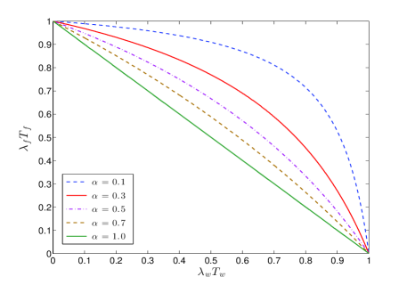
Figure 1: The minimum $\lambda_{f}T_{f}$ required for existence of a giant component in $\mathbb{H}(n;\alpha,T_{w}\lambda_{w},T_{f}\lambda_{f})$ versus $\lambda_{w}T_{w}$ for various $\alpha$ values. In other words, each curve corresponds to the boundary of the phase transition for the corresponding $\alpha$ value. Above the boundary there exists a giant component, but below it all components have $O(\log n)$ nodes.

We observe that the threshold function $\lambda_{fw}^{\star}$ is symmetric in $T_{f}\lambda_{f}$ and $T_{w}\lambda_{w}$, meaning that both networks have identical roles in carrying the conjoined network to the supercritical regime where information can reach a linear fraction of the nodes. To get a more concrete sense, we depict in Figure 1 the minimum $\lambda_{f}T_{f}$ required to have a giant component in $\mathbb{H}(n;\alpha,T_{w}\lambda_{w},T_{f}\lambda_{f})$ versus $\lambda_{w}T_{w}$ for various $\alpha$ values. Each curve in the figure corresponds to a phase transition boundary above which information epidemics are possible. If $T_{f}=T_{w}=1$, the same plot shows the boundary of the giant component existence with respect to the mean degrees $\lambda_{f}$ and $\lambda_{w}$. This clearly shows how two networks that are in the subcritical regime can yield an information epidemic when they are conjoined. For instance, we see that for $\alpha=0.1$, it suffices to have $\lambda_{f}=\lambda_{w}=0.76$ for the existence of an information epidemic. Yet, if the two networks were disjoint, it would be necessary [33] to have $\lambda_{f}>1$ and $\lambda_{w}>1$.

We elaborate further on Theorem 3.3. First, we note from the classical results [33] that ER graphs have a giant component whenever average node degree exceeds one. This is compatible with part $(i)$ of Theorem 3.3, since the condition for giant component existence reduces to $T_{f}\lambda_{f}>1$ if $T_{w}\lambda_{w}=0$ and $T_{w}\lambda_{w}>1$ when $T_{f}\lambda_{f}=0$. Finally, in the case where $\alpha=1$ (i.e., when everyone in the population is a member of Facebook), the graph $\mathbb{H}$ reduces to an ER graph with edge probability $\frac{T_{f}\lambda_{f}+T_{w}\lambda_{w}-\frac{T_{f}T_{w}\lambda_{f}\lambda_{w}}{n}}{n}$ leading to a mean node degree of $T_{f}\lambda_{f}+T_{w}\lambda_{w}$ in the asymptotic regime. As expected, for the case $\alpha=1$, Theorem 3.3 reduces to classical results for ER graphs as we see that $\lambda_{fw}^{\star}=T_{f}\lambda_{f}+T_{w}\lambda_{w}$ and $\frac{1}{n}C_{1}(\mathbb{H})\xrightarrow{p}\rho_{1}$ where $\rho_{1}$ is the largest solution of $\rho_{1}=1-e^{-\rho_{1}(T_{f}\lambda_{f}+T_{w}\lambda_{w})}.$

IV Numerical Results

IV-A ER Networks

We first study the case where both the physical information network $\mathbb{W}$ and the online social network $\mathbb{F}$ are Erdős-Rényi graphs. As in Section III-B, let $\mathbb{H}(n;\alpha,T_{w}\lambda_{w},T_{f}\lambda_{f})=\mathbb{W}(n;T_{w}\lambda_{w}/n)\cup\mathbb{F}(n;\alpha,T_{f}\lambda_{f}/(\alpha n))$ be the conjoint social-physical network, where $\mathbb{W}$ is defined on the vertices $\{1,\ldots,n\}$, whereas the vertex set of $\mathbb{F}$ is obtained by picking each node $1,\ldots,n$ independently with probability $\alpha$. The information transmissibilities are equal to $T_{w}$ and $T_{f}$ in $\mathbb{W}$ and $\mathbb{F}$, respectively, so that the mean degrees are given (asymptotically) by $T_{w}\lambda_{w}$ and $T_{f}\lambda_{f}$, respectively.

We plot in Figure 2 the fractional size of the giant component in $\mathbb{H}(n;\alpha,T_{w}\lambda_{w},T_{f}\lambda_{f})$ versus $T_{f}\lambda_{f}=T_{w}\lambda_{w}$ for various $\alpha$ values. In other words, the plots illustrate the largest fraction of individuals that a particular item of information can reach. In this figure, the curves stand for the analytical results obtained by Theorem 3.3 whereas marked points stand for the experimental results obtained with $n=2\times 10^{5}$ nodes by averaging $200$ experiments for each data point. Clearly, there is an excellent match between the theoretical and experimental results. It is also seen that the critical threshold for the existence of a giant component (i.e., an information epidemic) is given by $T_{f}\lambda_{f}=T_{w}\lambda_{w}=0.760$ when $\alpha=0.1$, $T_{f}\lambda_{f}=T_{w}\lambda_{w}=0.586$ when $\alpha=0.5$, and $T_{f}\lambda_{f}=T_{w}\lambda_{w}=0.514$ when $\alpha=0.9$. It is easy to check that these values are in perfect agreement with the theoretically obtained critical threshold $\lambda_{fw}^{\star}$ given by (III-B).

In the inset of Figure 2, we demonstrate the average outbreak size $<s>$ versus $T_{f}\lambda_{f}=T_{w}\lambda_{w}$ under the same setting. Namely, the curves stand for the analytical results obtained from Theorem 13, while the marked points are obtained by averaging the quantity given in (10) over 200 independent experiments. We see that experimental results are in excellent agreement with our analytical results. Also, as expected, average outbreak size $<s>$ is seen to grow unboundedly as $T_{f}\lambda_{f}=T_{w}\lambda_{w}$ approaches to the corresponding epidemic threshold.

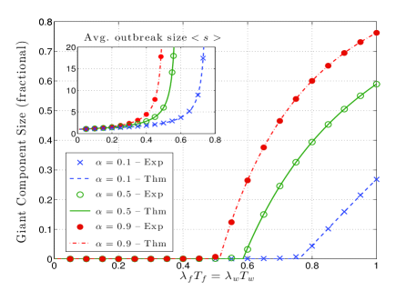
Figure 2: The fractional size of the giant component in $\mathbb{H}(n;\alpha,T_{w}\lambda_{w},T_{f}\lambda_{f})$ versus $T_{f}\lambda_{f}=T_{w}\lambda_{w}$. The curves correspond to analytical results obtained from Theorem 3.3, whereas marked points stand for the experimental results obtained with $n=2\times 10^{5}$ by averaging $200$ experiments for each point. (Inset) Average out-break size $<s>$ versus $T_{f}\lambda_{f}=T_{w}\lambda_{w}$ under the same setting.

IV-B Networks with Power Degree Distributions

In order to gain more insight about the consequences of Theorem 3.1 for real-world networks, we now consider a specific example of information diffusion when the physical information network $\mathbb{W}$ and the online social network $\mathbb{F}$ have power-law degree distributions with exponential cutoff. Specifically, we let

$$p_{k}^{w}=\left\{\begin{array}[]{ll}0&\textrm{if $k=0$}\\ \left(\mbox{Li}_{\gamma_{w}}(e^{-1/\Gamma_{w}})\right)^{-1}k^{-\gamma_{w}}e^{-k/\Gamma_{w}}&\textrm{if $k=1,2,\ldots$}\\ \end{array}\right.$$ (16)

and

$$p_{k}^{f}=\left\{\begin{array}[]{ll}0&\textrm{if $k=0$}\\ \left(\mbox{Li}_{\gamma_{f}}(e^{-1/\Gamma_{f}})\right)^{-1}k^{-\gamma_{f}}e^{-k/\Gamma_{f}}&\textrm{if $k=1,2,\ldots$},\\ \end{array}\right.$$ (17)

where $\gamma_{w}$, $\gamma_{f}$, $\Gamma_{w}$ and $\Gamma_{f}$ are positive constants and the normalizing constant $\mbox{Li}_{m}(z)$ is the $m$th polylogarithm of $z$; i.e., $\mbox{Li}_{m}(z)=\sum_{k=1}^{\infty}\frac{z^{k}}{k^{m}}.$

Power law distributions with exponential cutoff are chosen here because they are applied to a variety of real-world networks [20, 27]. In fact, a detailed empirical study on the degree distributions of real-world networks [34] revealed that the Internet (at the level of autonomous systems), the phone call network, the e-mail network, and the web link network all exhibit power law degree distributions with exponential cutoff.

To apply Theorem 3.1, we first compute the epidemic threshold given by (III-A). Under (16)-(17) we find that

$$\lambda_{f} = \frac{\mbox{Li}_{\gamma_{f}-1}(e^{-1/\Gamma_{f}})}{\mbox{Li}_{\gamma_{f}}(e^{-1/\Gamma_{f}})},$$

$$\beta_{f} = \frac{\mbox{Li}_{\gamma_{f}-2}(e^{-1/\Gamma_{f}})-\mbox{Li}_{\gamma_{f}-1}(e^{-1/\Gamma_{f}})}{\mbox{Li}_{\gamma_{f}-1}(e^{-1/\Gamma_{f}})}$$

Similar expressions can be derived for $\lambda_{w}$ and $\beta_{w}$. It is now a simple matter to compute the critical threshold $\sigma_{fw}^{\star}$ from (III-A) using the above relations. Then, we can use Theorem 3.1(i) to check whether or not an item of information can reach a linear fraction of individuals in the conjoint social-physical network $\mathbb{H}(n;\alpha,\{p_{k}^{w}\},T_{w},\{p_{k}^{f}\},T_{f})=\mathbb{W}(n;\{p_{k}^{w}\},T_{w})\cup\mathbb{F}(n;\alpha,\{p_{k}^{f}\},T_{f})$.

To that end, we depict in Figure 3 the minimum $T_{f}$ value required to have a giant component in $\mathbb{H}(n;\alpha,\{p_{k}^{w}\},T_{w},\{p_{k}^{f}\},T_{f})$ versus $T_{w}$, for various $\alpha$ values. In other words, each curve corresponds to a phase transition boundary above which information epidemics are possible, in the sense that an information has a positive probability of reaching out to a linear fraction of individuals in the overlaying social-physical network. In all plots, we set $\gamma_{f}=\gamma_{w}=2.5$ and $\Gamma_{f}=\Gamma_{w}=10$. The $T_{f}$ and $T_{w}$ values are multiplied by the corresponding $\beta_{f}$ and $\beta_{w}$ values to make a fair comparison with the disjoint network case where it is required [20] to have $\beta_{w}T_{w}>1$ (or $\beta_{f}T_{f}>1$) for the existence of an epidemic; under the current setting we have $\beta_{f}=\beta_{w}=1.545$. Figure 3 illustrates how conjoining two networks can speed up the information diffusion. It can be seen that even for small $\alpha$ values, two networks, albeit having no giant component individually, can yield an information epidemic when they are conjoined. As an example, we see that for $\alpha=0.1$, it suffices to have that $\beta_{f}T_{f}=\beta_{w}T_{w}=0.774$ for the existence of an information epidemic in the conjoint network $\mathbb{H}$, whereas if the networks $\mathbb{W}$ and $\mathbb{F}$ are disjoint, an information epidemic can occur only if $\beta_{w}T_{w}>1$ or $\beta_{f}T_{f}>1$.

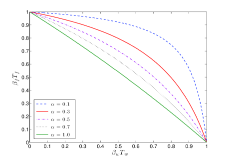
Figure 3: The minimum $T_{f}$ required for the existence of a giant component in $\mathbb{H}(n;\alpha,\{p_{k}^{w}\},T_{w},\{p_{k}^{f}\},T_{f})$ versus $T_{w}$. The distributions $\{p_{k}^{w}\}$ and $\{p_{k}^{f}\}$ are given by (16) and (17), with $\gamma_{f}=\gamma_{w}=2.5$ and $\Gamma_{f}=\Gamma_{w}=10$. The $T_{f}$ and $T_{w}$ values are multiplied by the corresponding $\beta_{f}$ and $\beta_{w}$ values to provide a fair comparison with the disjoint network case; under the current setting we have $\beta_{f}=\beta_{w}=1.545$.

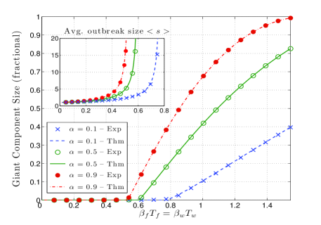
Figure 4: The fractional size of the giant component in $\mathbb{H}(n;\alpha,\{p_{k}^{w}\},T_{w},\{p_{k}^{f}\},T_{f})$ versus $T_{f}\beta_{f}=T_{w}\beta_{w}$. The distributions $\{p_{k}^{w}\}$ and $\{p_{k}^{f}\}$ are given by (16) and (17), with $\gamma_{f}=\gamma_{w}=2.5$ and $\Gamma_{f}=\Gamma_{w}=10$. The $T_{f}$ and $T_{w}$ values are multiplied by the corresponding $\beta_{f}$ and $\beta_{w}$ values for fair comparison with the disjoint network case; under the current setting we have $\beta_{f}=\beta_{w}=1.545$. The curves were obtained analytically via Theorem 3.1, whereas the marked points stand for the experimental results obtained with $n=2\times 10^{5}$ nodes by averaging $200$ experiments for each parameter set. We see that there is an excellent agreement between theory and experiments. (Inset) Average out-break size $<s>$ versus $\beta_{f}T_{f}=\beta_{w}T_{w}$ under the same setting.

Next, we turn to computation of the giant component size. We note that

$$\begin{array}[]{c}{\mathbb{E}}\left[{h_{1}^{k_{f}}}\right]=\frac{\mbox{Li}_{\gamma_{f}}(h_{1}e^{-1/\Gamma_{f}})}{\mbox{Li}_{\gamma_{f}}(e^{-1/\Gamma_{f}})}\\ {\mathbb{E}}\left[{k_{f}h_{1}^{k_{f}-1}}\right]=\frac{\mbox{Li}_{\gamma_{f}-1}(h_{1}e^{-1/\Gamma_{f}})}{\mbox{Li}_{\gamma_{f}}(e^{-1/\Gamma_{f}})h_{1}}.\end{array}$$

and similar expressions can be derived for $\mathbb{E}[h_{2}^{k_{w}}]$ and $\mathbb{E}[k_{w}h_{2}^{k_{w}-1}]$. Now, for any given set of parameters, $\gamma_{f},\gamma_{w},T_{f},T_{w},\Gamma_{f},\Gamma_{w},\alpha$, we can numerically obtain the giant component size of $\mathbb{H}(n;\alpha,\{p_{k}^{w}\},T_{w},\{p_{k}^{f}\},T_{f})$ by invoking the above relations into part $(ii)$ of Theorem 3.1.

To this end, Figure 4 depicts the fractional size of the giant component in $\mathbb{H}(n;\alpha,\{p_{k}^{w}\},T_{w},\{p_{k}^{f}\},T_{f})$ versus $T_{f}\beta_{f}=T_{w}\beta_{w}$, for various $\alpha$ values; as before, we set $\gamma_{f}=\gamma_{w}=2.5$ and $\Gamma_{f}=\Gamma_{w}=10$ yielding $\beta_{f}=\beta_{w}=1.545$. In other words, the plots stand for the largest fraction of individuals in the social-physical network who receive an information item that has started spreading from a single individual. In Figure 4, the curves were obtained analytically via Theorem 3.1 whereas the marked points stand for the experimental results obtained with $n=2\times 10^{5}$ nodes by averaging $200$ experiments for each parameter set. We see that there is an excellent agreement between theory and experiment. Moreover, according to the experiments, the critical threshold for the existence of a giant component (i.e., an information epidemic) appears at $T_{f}\beta_{f}=T_{w}\beta_{w}=0.78$ when $\alpha=0.1$, $T_{f}\beta_{f}=T_{w}\beta_{w}=0.61$ when $\alpha=0.5$, and $T_{f}\beta_{f}=T_{w}\beta_{w}=0.53$ when $\alpha=0.9$. These values are in perfect agreement with the theoretically obtained critical threshold $\sigma_{fw}^{\star}$ given by (III-A).

The inset of Figure 4 shows the average outbreak size $<s>$ versus $\beta_{f}T_{f}=\beta_{w}T_{w}$ under the same setting. To avoid the finite size effect (observed by Newman [20] as well) near the epidemic threshold, we have increased the network size up to $n=30\times 10^{6}$ to obtain a better fit. Again, we see that experimental results (obtained by averaging the quantity (10) over 200 independent experiments) agree well with the analytical results of Theorem 13.

V Online Social Networks with $o(n)$ nodes

Until now, we have assumed that apart from the physical network $\mathbb{W}$ on $n$ nodes, information can spread over an online social network which has $\Omega(n)$ members. However, one may also wonder as to what would happen if the number of nodes in the online network is a sub-linear fraction of $n$. For instance, consider an online social network $\mathbb{F}$ whose vertices are selected by picking each node $1,\ldots,n$ with probability $n^{\gamma-1}$ where $0<\gamma<1$. This would yield a vertex set $\mathcal{N}_{F}$ that satisfies

$$|\mathcal{N}_{F}|\leq n^{\gamma}(1+\epsilon)$$ (18)

with high probability for any $\epsilon>0$. We now show that, asymptotically, social networks with $n^{\gamma}$ nodes have almost no effect in spreading information. We start by establishing an upper bound on the size of the giant component in $\mathbb{H}=\mathbb{W}\cup\mathbb{F}$.

Proposition 5.1

Let $\mathbb{W}$ be a graph on vertices $1,\ldots,n$, and $\mathbb{F}$ be a graph on the vertex set $\mathcal{N}_{F}\subset\{1,\ldots,n\}$. With $\mathbb{H}=\mathbb{W}\cup\mathbb{F}$, we have

$$C_{1}(\mathbb{H})\leq C_{1}(\mathbb{W})+C_{2}(\mathbb{W})(|\mathcal{N}_{F}|-1),$$ (19)

where $C_{1}(\mathbb{W})$ and $C_{2}(\mathbb{W})$ are sizes of the first and second largest components of $\mathbb{W}$, respectively.

Proof:

It is clear that $C_{1}(\mathbb{H})$ will take its largest value when $\mathbb{F}$ is a fully connected graph; i.e., a graph with edges between every pair of vertices. In that case the largest component of $\mathbb{H}$ can be obtained by taking a union of the largest components of $\mathbb{W}$ that can be reached from the nodes in $\mathcal{N}_{F}$. With $C_{1}^{i}(\mathbb{W})$ denoting set of nodes in the largest component (of $\mathbb{W}$) that can be reached from node $i$, we have

$$C_{1}(\mathbb{H})=\left|\cup_{i\in\mathcal{N}_{F}}C_{1}^{i}(\mathbb{W})\right|\leq C_{1}(\mathbb{W})+C_{2}(\mathbb{W})+\ldots C_{|\mathcal{N}_{F}|}(\mathbb{W})$$ (20)

where $C_{j}(\mathbb{W})$ stands for the $j$th largest component of $\mathbb{W}$. The inequality (20) is easy to see once we write

$$\left|\cup_{i\in\mathcal{N}_{F}}C_{1}^{i}(\mathbb{W})\right|=\sum_{i=1}^{|\mathcal{N}_{F}|}\left|C_{1}^{\mathcal{N}_{F}(i)}(\mathbb{W})-\bigcup_{j=1}^{i-1}C_{1}^{\mathcal{N}_{F}(j)}(\mathbb{W})\right|$$

where $\mathcal{N}_{F}(i)$ is the $i$th element of $\mathcal{N}_{F}$. The above quantity is a summation of the sizes of $|\mathcal{N}_{F}|$ mutually disjoint components of $\mathbb{W}$. As a result, this summation can be no larger than the sum of the first $|\mathcal{N}_{F}|$ largest components of $\mathbb{W}$. The desired conclusion (19) is now immediate as we note that $C_{2}(\mathbb{W})\geq C_{j}(\mathbb{W})$ for all $j=3,\ldots,\mathcal{N}_{F}$. ∎

The next result is an easy consequence of Proposition 5.1 and classical results [33] for ER graphs.

Corollary 5.1

Let $\mathbb{W}$ be an ER graph on the vertices $1,\ldots,n$ and let $\mathbb{F}$ be a graph whose vertex set $\mathcal{N}_{F}$ satisfies (18) whp. The followings hold for $\mathbb{H}=\mathbb{W}\cup\mathbb{F}$:

• If $\mathbb{W}$ is in the subcritical regime (i.e., if $C_{1}(\mathbb{W})=o(n)$), then whp we have $C_{1}(\mathbb{H})=o(n)$.

• If $C_{1}(\mathbb{W})=\Theta(n)$, then we have

  $$C_{1}(\mathbb{H})=(1+o(1))C_{1}(\mathbb{W}).$$

Proof:

It is known [33] that for an ER graph $\mathbb{W}$, it either holds that $C_{1}(\mathbb{W})=O(\log n)$ (subcritical regime) or it is the case that $C_{1}(\mathbb{W})=\Theta(n)$ while $C_{2}(\mathbb{W})=O(\log n)$ (supercritical regime). Under condition (18), we see from (19) that whenever $C_{1}(\mathbb{W})=o(n)$ we have $C_{1}(\mathbb{H})\leq c\log n\cdot n^{\gamma}$ for some $c>0$ and part $(i)$ follows immediately. Next, assume that we have $C_{1}(\mathbb{W})=\Theta(n)$. The claim $(ii)$ follows from (19) as we note that

$$\lim_{n\to\infty}\frac{C_{2}(\mathbb{W})\cdot n^{\gamma}}{C_{1}(\mathbb{W})}=0$$

since $C_{2}(\mathbb{W})=O(\log n)$. ∎

Corollary 5.1 shows that in the case where only a sub-linear fraction of the population use online social networks, an information item originating at a particular node can reach a positive fraction of individuals if and only if information epidemics are already possible in the physical information network. Moreover, we see from Corollary 5.1 that the fractional size of a possible information epidemic in the conjoint social-physical network is the same as that of the physical information network alone. Combining these, we conclude that online social networks with $n^{\gamma}$ ($0\leq\gamma<1$) members have no effect on the (asymptotic) fraction of individuals that can be influenced by an information item in the conjoint social-physical network.

Along the same line as in Corollary 5.1, we next turn our attention to random graphs $\mathbb{W}$ with arbitrary degree distribution [31, 35]. This time we rely on the results by Molloy and Reed [35, Theorem 1] who have shown that if there exists some $\epsilon>0$ such that

$$\max\{d_{i},i=1,\ldots,n\}\leq n^{\frac{1}{4}-\epsilon}$$ (21)

then in the supercritical regime (i.e., when $C_{1}(\mathbb{W})=\Theta(n)$) we have $C_{2}(\mathbb{W})=O(\log n)$. It was also shown [35] that in the subcritical regime of the phase transition, we have $C_{1}(\mathbb{W})=O(w(n)^{2}\log n)$ whenever

$$\max\left\{d_{i},i=1,\ldots,n\right\}\leq w(n)$$ (22)

with $w(n)\leq n^{\frac{1}{8}-\epsilon}$ for some $\epsilon>0$.

Now, consider a graph $\mathbb{F}$ whose vertex set $\mathcal{N}_{F}$ satisfies (18) whp and let $\mathbb{W}$ be a random graph with a given degree sequence $\{d_{i}\}_{i=1}^{n}$ satisfying (21). In view of (19), it is easy to see that

$$C_{1}(\mathbb{H})=(1+o(1))C_{1}(\mathbb{W})$$

where $\mathbb{H}=\mathbb{W}\cup\mathbb{F}$ and this provides an analog of Corollary 5.1(ii). It is also immediate that in the subcritical regime, we have

$$C_{1}(\mathbb{H})=o(n)$$

as long as (22) is satisfied and (18) holds for some $\gamma\leq\frac{3}{4}$; this establishes an analog of Corollary 5.1(i) for graphs with arbitrary degree distributions.

The above result takes a simpler form for classes of random graphs $\mathbb{W}$ studied in Section IV-B; i.e., random graphs where the degrees follow a power-law distribution with exponential cutoff. In particular, let the degrees of $\mathbb{W}$ be distributed according to (16). It is easy to see that

$$\max\{d_{i},i=1,\ldots,n\}=O(\log n)$$

with high probability so that conditions (21) and (22) are readily satisfied. For the latter condition, it suffices to take $w_{n}=O(\log n)$ so that in the subcritical regime, we have

$$C_{1}(\mathbb{W})=O\left((\log n)^{3}\right).$$

The next corollary is now an immediate consequence of Proposition 5.1.

Corollary 5.2

Let $\mathbb{W}$ be a random graph whose degrees follow the distribution specified in (16) and let $\mathbb{F}$ be a graph whose vertex set $\mathcal{N}_{F}$ satisfies (18) whp. The followings hold for $\mathbb{H}=\mathbb{W}\cup\mathbb{F}$:

• If $C_{1}(\mathbb{W})=o(n)$, then whp we have $C_{1}(\mathbb{H})=o(n)$.

• If $C_{1}(\mathbb{W})=\Theta(n)$, then we have

  $$C_{1}(\mathbb{H})=(1+o(1))C_{1}(\mathbb{W}).$$

VI Proofs of Theorem 3.1 and Theorem 13

Consider random graphs $\mathbb{W}(n,\{p_{k}^{w}\})$ and $\mathbb{F}(n;\alpha,\{p_{k}^{f}\})$ as in Section III-A. In order to study the diffusion of information in the overlay network $\mathbb{H}=\mathbb{W}\cup\mathbb{F}$, we consider a branching process which starts by giving a piece of information to an arbitrary node, and then recursively reveals the largest number of nodes that are reached and informed by exploring its neighbors. We remind that information propagates from a node to each of its neighbors independently with probability $T_{f}$ through links in $\mathbb{F}$ (type-$1$) and with probability $T_{w}$ through links in $\mathbb{W}$ (type-$2$). In the following, we utilize the standard approach on generating functions [31, 20], and determine the condition for the existence of a giant informed component as well as the final expected size of the information epidemics. This approach is valid long as the initial stages of the branching process is locally tree-like, which holds in this case as the clustering coefficient of colored degree-driven networks scales like $1/n$ as $n$ gets large [39].

We now solve for the survival probability of the aforementioned branching process by using the mean-field approach based on the generating functions [31, 20]. Let $h_{1}(x)$ (resp. $h_{2}(x)$) denote the generating functions for the finite number of nodes reached and informed by following a type-$1$ (resp. type-$2$) edge in the above branching process. In other words, we let $h_{1}(x)=\sum v_{m}x^{m}$ where $v_{m}$ is the “probability that an arbitrary type-$1$ link leads to a finite informed component of size $m$”; $h_{2}(x)$ is defined analogously for type-$2$ links. Finally, we let $H(x)$ define the generating function for the finite number of nodes that receive an information started from an arbitrary node.

We start by deriving the recursive relations governing $h_{1}(x)$ and $h_{2}(x)$. We find that the generating functions $h_{1}(x)$ and $h_{2}(x)$ satisfy the self-consistency equations

$$h_{1}(x)=x\sum_{\boldsymbol{d}}\frac{d_{f}p_{\boldsymbol{d}}}{<d_{f}>}T_{f}h_{1}(x)^{d_{f}-1}h_{2}(x)^{d_{w}}+(1-T_{f})\hskip 2.84526pt$$ (23)

$$h_{2}(x)=x\sum_{\boldsymbol{d}}\frac{d_{w}p_{\boldsymbol{d}}}{<d_{w}>}T_{w}h_{1}(x)^{d_{f}}h_{2}(x)^{d_{w}-1}+(1-T_{w})$$ (24)

The validity of (23) can be seen as follows: The explicit factor $x$ accounts for the initial vertex that is arrived at. The factor $d_{f}p_{\boldsymbol{d}}/<d_{f}>$ gives [20] the normalized probability that an edge of type $1$ is attached (at the other end) to a vertex with colored degree $\boldsymbol{d}=(d_{f},d_{w})$. Since the arrived node is reached by a type-$1$ link, it will receive the information with probability $T_{f}$. If the arrived node receives the information, it will be added to the component of informed nodes and it can inform other nodes via its remaining $d_{f}-1$ links of type-$1$ and $d_{w}$ links of type-$2$. Since the number of nodes reached and informed by each of its type-$1$ (resp. type-$2$) links is generated in turn by $h_{1}(x)$ (resp. $h_{2}(x)$) we obtain the term $h_{1}(x)^{d_{f}-1}h_{2}(x)^{d_{w}}$ by the powers property of generating functions [31, 20]. Averaging over all possible colored degrees $\boldsymbol{d}$ gives the first term in (23). The second term with the factor $x^{0}=1$ accounts for the possibility that the arrived node does not receive the information and thus is not included in the cluster of informed nodes. The relation (24) can be validated via similar arguments.

Using the relations (23)-(24), we now find the finite number of nodes reached and informed by the above branching process. We have that

$$H(x)=x\sum_{\boldsymbol{d}}p_{\boldsymbol{d}}h_{1}(x)^{d_{f}}h_{2}(x)^{d_{w}}.$$ (25)

Similar to (23)-(24), the relation (25) can be seen as follows: The factor $x$ corresponds to the initial node that is selected arbitrarily and given a piece of information. The selected node has colored degree $\boldsymbol{d}=(d_{f},d_{w})$ with probability $p_{\boldsymbol{d}}$. The number of nodes it reaches and informs via each of its $d_{f}$ (resp. $d_{w}$) links of type $1$ (resp. type $2$) is generated by $h_{1}(x)$ (resp. $h_{2}(x)$). This yields the term $h_{1}(x)^{d_{f}}h_{2}(x)^{d_{w}}$ and averaging over all possible colored degrees, we get (25).

We are interested in the solution of the recursive relations (23)-(24) for the case $x=1$. This case exhibits a trivial fixed point $h_{1}(1)=h_{2}(1)=1$ which yields $H(1)=1$ meaning that the underlying branching process is in the subcritical regime and that all informed components have finite size as understood from the conservation of probability. However, the fixed point $h_{1}(1)=h_{2}(1)=1$ corresponds to the physical solution only if it is an attractor; i.e., a stable solution to the recursion (23)-(24). The stability of this fixed point can be checked via linearization of (23)-(24) around $h_{1}(1)=h_{2}(1)=1$, which yields the Jacobian matrix $\boldsymbol{J}$ given by $\boldsymbol{J}(i,j)=\frac{\partial h_{i}(1)}{\partial h_{j}(1)}\big{|}_{h_{1}(1)=h_{2}(1)=1}$ for $i,j=1,2$. This gives

$$\boldsymbol{J}=\left[\begin{array}[]{cc}\frac{T_{f}<(d_{f}^{2}-d_{f})>}{<d_{f}>}&\frac{T_{f}<d_{f}d_{w}>}{<d_{f}>}\\ &\\ \frac{T_{w}<d_{w}d_{f}>}{<d_{w}>}&\frac{T_{w}<(d_{w}^{2}-d_{w})>}{<d_{w}>}\end{array}\right].$$ (26)

If all the eigenvalues of $\boldsymbol{J}$ are less than one in absolute value (i.e., if the spectral radius $\sigma(\boldsymbol{J})$ of $\boldsymbol{J}$ satisfies $\sigma(\boldsymbol{J})\leq 1$), then the solution ${h}_{1}(1)=h_{2}(1)=1$ is an attractor and $H(1)=1$ becomes the physical solution, meaning that $\mathbb{H}(n;\alpha,\{p^{w}_{k}\},T_{w},\{p^{f}_{k}\},T_{f})$ does not possess a giant component whp. In that case, the fraction of nodes that receive the information tends to zero in the limit $n\to\infty$. On the other hand, if the spectral radius of $\boldsymbol{J}$ is larger than one, then the fixed point ${h}_{1}(1)=h_{2}(1)=1$ is unstable pointing out that the asymptotic branching process is supercritical, with a positive probability of producing infinite trees. In that case, a nontrivial fixed point exists and becomes the attractor of the recursions (23)-(24), yielding a solution with $h_{1}(1),h_{2}(1)<1$. In view of (25) this implies $H(1)<1$ and the corresponding probability deficit $1-H(1)$ is attributed to the existence of a giant (infinite) component of informed nodes. In fact, the quantity $1-H(1)$ is equal to the probability that a randomly chosen vertex belongs to the giant component, which contains asymptotically a fraction $1-H(1)$ of the vertices.

Collecting these Theorem 3.1 is now within easy reach. First, recall that $k_{f}$ and $k_{w}$ are random variables independently drawn from the distributions $\{p_{k}^{f}\}$ and $\{p_{k}^{w}\}$, respectively, so that $d_{f}$ is a random variable that is statistically equivalent to $k_{f}$ with probability $\alpha$, and equal to zero otherwise. On the other hand, we have $k_{w}\buildrel st\over{=}d_{w}$. Using (4) in (26), we now get

$$\boldsymbol{J}=\left[\begin{array}[]{cc}T_{f}\beta_{f}&T_{f}\lambda_{w}\\ T_{w}\alpha\lambda_{f}&T_{w}\beta_{w}\end{array}\right]$$

by the independence of $d_{f}$ and $d_{w}$. It is now a simple matter to see that $\sigma(\boldsymbol{J})=\sigma_{fw}^{\star}$, where $\sigma_{fw}^{\star}$ is as defined in (III-A). Therefore, we have established that the epidemic threshold is given by $\sigma_{fw}^{\star}=1$, and part (i) of Theorem 3.1 follows.

Next, we set $x=1$ in the recursive relations (23)-(24) and let $h_{1}:=h_{1}(1)$ and $h_{2}:=h_{2}(1)$. Using (3) and elementary algebra, we find that the stable solution of the recursions (23)-(24) is given by the smallest solution of (6)-(7) with $h_{1},h_{2}$ in $(0,1]$. It is also easy to check from (25) that

$$H(1)={\mathbb{E}}\left[{\alpha h_{1}^{k_{f}}+1-\alpha}\right]\times{\mathbb{E}}\left[{h_{2}^{k_{w}}}\right],$$

and part (ii) of Theorem 3.1 follows upon recalling that the fractional size of the giant component (i.e., the number of informed nodes) is given by $1-H(1)$ whp.

We now turn to proving Theorem 13. In the subcritical regime, $H(x)$ corresponds to generating function for the distribution of outbreak sizes; i.e, distribution of the number of nodes that receive an information started from an arbitrary node. Therefore, the mean outbreak size is given by the first derivative of $H(x)$ at the point $x=1$. Namely, we have

$$<s>=\frac{dH(x)}{dx}\Big{|}_{x=1}:=H^{\prime}(1).$$ (27)

Recalling that $h_{1}(1)=h_{2}(1)=1$ in the subcritical regime, we get from (25) that

$$H^{\prime}(1) = 1+h_{1}^{\prime}(1)\sum_{\boldsymbol{d}}p_{\boldsymbol{d}}d_{f}+h_{2}^{\prime}(1)\sum_{\boldsymbol{d}}p_{\boldsymbol{d}}d_{w}$$ (28)

$$= 1+\alpha\lambda_{f}h_{1}^{\prime}(1)+\lambda_{w}h_{2}^{\prime}(1).$$

The derivatives $h_{1}^{\prime}(1)$ and $h_{2}^{\prime}(1)$ can also be computed recursively using the relations (23)-(24). In fact, it is easy to check that

$$h_{1}^{\prime}(1) = T_{f}+T_{f}\beta_{f}h_{1}^{\prime}(1)+T_{f}\lambda_{w}h_{2}^{\prime}(1)$$ (29)

$$h_{2}^{\prime}(1) = T_{w}+T_{w}\alpha\lambda_{f}h_{1}^{\prime}(1)+T_{w}\beta_{w}h_{2}^{\prime}(1)$$ (30)

upon using (4) and other definitions introduced previously. Now, setting $s_{1}:=h_{1}^{\prime}(1)$ and $s_{2}:=h_{2}^{\prime}(1)$, we obtain (11)-(12) from (29)-(30), and Theorem 13 follows upon substituting (28) into (27).

VII Proof of Theorem 3.3

In this section, we give a proof Theorem 3.3. First, we summarize the technical tools that will be used.

VII-A Inhomogeneous Random Graphs

Recently, Bollobas, Janson and Riordan [38] have developed a new theory of inhomogeneous random graphs that would allow studying phase transition properties of complex networks in a rigorous fashion. The authors in [38] established very general results for various properties of these models, including the critical point of their phase transition, as well as the size of their giant component. Here, we summarize these tools with focus on the results used in this paper.

At the outset, assume that a graph is defined on vertices $\{1,\ldots,n\}$, where each vertex $i$ is assigned randomly or deterministically a point $x_{i}$ in a metric space $S$. Assume that the metric space $S$ is equipped with a Borel probability measure $\mu$ such that for any $\mu$-continuity set $A\subseteq S$ (see [38])

$$\frac{1}{n}\cdot\sum_{i=1}^{n}{\bf 1}\left[x_{i}\in A\right]\xrightarrow{p}\mu(A).$$ (31)

A vertex space $\mathcal{V}$ is then defined as a triple $(S,\mu,\{x_{1},\ldots,x_{n}\})$ where $\{x_{1},\ldots,x_{n}\}$ is a sequence of points in $S$ satisfying (31).

Next, let a kernel $\kappa$ on the space $(S,\mu)$ define a symmetric, non-negative, measurable function on $S\times S$. The random graph $G^{\mathcal{V}}(n,\kappa)$ on the vertices $\{1,\ldots,n\}$ is then constructed by assigning an edge between $i$ and $j$ ($i<j$) with probability $\kappa(x_{i},x_{j})/n$, independently of all the other edges in the graph.

Consider random graphs $G^{\mathcal{V}}(n,\kappa)$ for which the kernel $\kappa$ is bounded and continuous a.e. on $S\times S$. In fact, in this study it suffices to consider only the cases where the metric space $S$ consists of finitely many points, i.e., $S=\{1,\ldots,r\}$. Under these assumptions, the kernel $\kappa$ reduces to an $r\times r$ matrix, and $G^{\mathcal{V}}(n,\kappa)$ becomes a random graph with vertices of $r$ different types; e.g., vertices with/without Facebook membership, etc. Two nodes (in $G^{\mathcal{V}}(n,\kappa)$) of type $i$ and $j$ are joined by an edge with probability $n^{-1}\kappa(i,j)$ and the condition (31) reduces to

$$\frac{n_{i}}{n}\xrightarrow{p}\mu_{i},\quad i=1,\ldots,r,$$ (32)

where $n_{i}$ stands for the number of nodes of type $i$ and $\mu_{i}$ is equal to $\mu(\{i\})$.

As usual, the phase transition properties of $G^{\mathcal{V}}(n,\kappa)$ can be studied by exploiting the connection between the component structure of the graph and the survival probability of a related branching process. In particular, consider a branching process that starts with an arbitrary vertex and recursively reveals the largest component reached by exploring its neighbors. For each $i=1,\ldots,r$, we let $\rho(\kappa;i)$ denote the probability that the branching process produces infinite trees when it starts with a node of type $i$. The survival probability $\rho(\kappa)$ of the branching process is then given by

$$\rho(\kappa)=\sum_{i=1}^{r}\rho(\kappa;i)\mu_{i}.$$ (33)

In analogy with the classical results for ER graphs [33], it is shown [38] that $\rho(\kappa;i)$’s satisfy the recursive equations

$$\rho(\kappa;i)=1-\exp\left\{-\sum_{j=1}^{r}\kappa(i,j)\mu_{j}\cdot\rho(\kappa;j)\right\},\>\>i=1,\ldots,r.$$ (34)

The value of $\rho(\kappa)$ can be computed via (33) by characterizing the stable fixed point of (34) reached from the starting point $\rho(\kappa;1)=\cdots=\rho(\kappa;r)=0$. It is a simple matter to check that, with $\boldsymbol{M}$ denoting an $r\times r$ matrix given by $\boldsymbol{M}(i,j)=\kappa(i,j)\cdot\mu_{j}$, the iterated map (34) has a non-trivial solution (i.e., a solution other than $\rho(\kappa;1)=\cdots=\rho(\kappa;r)=0$) iff

$$\sigma(\boldsymbol{M}):=\max\{|\lambda_{i}|:\lambda_{i}~{}\mbox{is~{}an~{}eigenvalue~{}of~{}$\boldsymbol{M}$}\}>1.$$ (35)

Thus, we see that if the spectral radius of $\boldsymbol{M}$ is less than or equal to one, the branching process is subcritical with $\rho(\kappa)=0$ and the graph $G^{\mathcal{V}}(n,\kappa)$ has no giant component; i.e., we have that $C_{1}(G^{\mathcal{V}}(n,\kappa))=o(n)$ whp.

On the other hand, if $\sigma(\boldsymbol{M})>1$, then the branching process is supercritical and there is a non-trivial solution $\rho(\kappa;i)>0,i=1,\ldots,r$ that corresponds to a stable fixed point of (34). In that case, $\rho(\kappa)>0$ corresponds to the probability that an arbitrary node belongs to the giant component, which asymptotically contains a fraction $\rho(\kappa)$ of the vertices. In other words, if $\sigma(\boldsymbol{M})>1$, we have that $C_{1}(G^{\mathcal{V}}(n,\kappa))=\Omega(n)$ whp, and $\frac{1}{n}C_{1}(G^{\mathcal{V}}(n,\kappa))\xrightarrow{p}\rho(\kappa)$.

Bollobas et al. [38, Theorem 3.12] have shown that the bound $C_{1}(G^{\mathcal{V}}(n,\kappa))=o(n)$ in the subcritical case can be improved under some additional conditions: They established that whenever $\sup_{i,j}\kappa(i,j)<\infty$ and $\sigma(\boldsymbol{M})\leq 1$, then we have $C_{1}(G^{\mathcal{V}}(n,\kappa))=O(\log n)$ whp as in the case of ER graphs. They have also shown that if either $\sup_{i,j}\kappa(i,j)<\infty$ or $\inf_{i,j}\kappa(i,j)>0$, then in the supercritical regime (i.e., when $\sigma(\boldsymbol{M})>1$) the second largest component satisfies $C_{2}(G^{\mathcal{V}}(n,\kappa))=O(\log n)$ whp.

VII-B A Proof of Theorem 3.3

We start by studying the information spread over the network $\mathbb{H}$ when information transmissibilities $T_{w}$ and $T_{f}$ are both equal to $1$. Clearly, this corresponds to studying the phase transition in $\mathbb{H}=\mathbb{H}(n;\alpha,\lambda_{w},\lambda_{f})$, and we will do so by using the techniques summarized in the previous section. Let $S=\{1,2\}$ stand for the space of vertex types, where vertices with Facebook membership are referred to as type $1$ while vertices without Facebook membership are said to be of type $2$; notice that this is different than the case in the proof of Theorem 3.1 where we distinguish between different link types. In other words, we let

$$x_{i}=\left\{\begin{array}[]{c}1\quad\textrm{if $i\in\mathcal{N}_{F}$}\\ 2\quad\textrm{if $i\not\in\mathcal{N}_{F}$}\\ \end{array}\right.$$

for each $i=1,\ldots,n$. Assume that the metric space $S$ is equipped with a probability measure $\mu$ that satisfies the condition (32); i.e., $\mu(\{1\}):=\mu_{1}=\alpha$ and $\mu(\{2\}):=\mu_{2}=1-\alpha$. Finally, we compute the appropriate kernel $\kappa$ such that, for each $i,j=\{1,2\}$, $\kappa(i,j)/n$ gives the probability that two vertices of type $i$ and $j$ are connected. Clearly, we have $\kappa(1,1)=n\left(1-\left(1-\frac{\lambda_{w}}{n}\right)\left(1-\frac{\lambda_{f}}{\alpha n}\right)\right)=\lambda_{w}+\frac{\lambda_{f}}{\alpha}-\frac{\lambda_{w}\lambda_{f}}{\alpha n}$, whereas $\kappa(1,2)=\kappa(2,1)=\kappa(2,2)=\lambda_{w}.$

We are now in a position to derive the critical point of the phase transition in $\mathbb{H}(n;\alpha,\lambda_{w},\lambda_{f})$ as well as the giant component size $C_{1}(\mathbb{H}(n;\alpha,\lambda_{w},\lambda_{f}))$. First, we compute the matrix $\boldsymbol{M}(i,j)=\kappa(i,j)\mu_{j}$ and get

$$\boldsymbol{M}=\left[\begin{array}[]{cc}\alpha\lambda_{w}+\lambda_{f}-\frac{\lambda_{w}\lambda_{f}}{n}&(1-\alpha)\lambda_{w}\\ \alpha\lambda_{w}&(1-\alpha)\lambda_{w}\\ \end{array}\right].$$

It is clear that the term $\frac{\lambda_{w}\lambda_{f}}{n}$ has no effect on the results as we eventually let $n$ go to infinity. It is now a simple matter to check that the spectral radius of $\boldsymbol{M}$ is given by

$$\sigma(\boldsymbol{M})=\frac{1}{2}\left(\lambda_{f}+\lambda_{w}+\sqrt{\left(\lambda_{f}+\lambda_{w}\right)^{2}-4(1-\alpha)\lambda_{f}\lambda_{w}}\right)$$

This leads to the conclusion that the random graph $\mathbb{H}(n;\alpha,\lambda_{w},\lambda_{f})$ has a giant component if and only if

$$\frac{1}{2}\left(\lambda_{f}+\lambda_{w}+\sqrt{\left(\lambda_{f}+\lambda_{w}\right)^{2}-4(1-\alpha)\lambda_{f}\lambda_{w}}\right)>1$$ (36)

as we recall (35). If condition (36) is not satisfied, then we have $C_{1}(\mathbb{H}(n;\alpha,\lambda_{w},\lambda_{f}))=O(\log n)$ as we note that $\sup_{i,j}\kappa(i,j)<\infty$. From [38, Theorem 3.12], we also get that $C_{2}(\mathbb{H}(n;\alpha,\lambda_{w},\lambda_{f}))=O(\log n)$ whenever (36) is satisfied.

Next, we compute the size of the giant component whenever it exists. Let $\rho(\kappa;1)=\rho_{1}$ and $\rho(\kappa;2)=\rho_{2}$. In view of (33) and the arguments presented previously, the asymptotic fraction of nodes in the giant component is given by

$$\rho(\kappa)=\alpha\rho_{1}+(1-\alpha)\rho_{2},$$ (37)

where $\rho_{1}$ and $\rho_{2}$ constitute a stable simultaneous solution of the transcendental equations

$$\begin{array}[]{l}\rho_{1}=1-\exp\left\{-\rho_{1}(\alpha\lambda_{w}+\lambda_{f})-\rho_{2}(1-\alpha)\lambda_{w}\right\}\\ \rho_{2}=1-\exp\left\{-\rho_{1}\alpha\lambda_{w}-\rho_{2}(1-\alpha)\lambda_{w}\right\}\\ \end{array}$$ (38)

So far, we have established the epidemic threshold and the size of the information epidemic when $T_{w}=T_{f}=1$. In the more general case where there is no constraint on the transmissibilities, we see that the online social network $\mathbb{F}$ becomes an ER graph with average degree $T_{f}\lambda_{f}$, whereas the physical network $\mathbb{W}$ becomes an ER graph with average degree $T_{w}\lambda_{w}$. Therefore, the critical threshold and the size of the information epidemic can be found by substituting $T_{f}\lambda_{f}$ for $\lambda_{f}$ and $T_{w}\lambda_{w}$ for $\lambda_{w}$ in the relations (36), (37) and (38). This establishes Theorem 3.3.

VIII Conclusion

In this paper, we characterized the critical threshold and the asymptotic size of information epidemics in an overlaying social-physical network. To capture the spread of information, we considered a physical information network that characterizes the face-to-face interactions of human beings, and some overlaying online social networks (e.g., Facebook, Twitter, etc.) that are defined on a subset of the population. Assuming that information is transmitted between individuals according to the SIR model, we showed that the critical point and the size of information epidemics on this overlaying social-physical network can be precisely determined.

To the best of our knowledge, this study marks the first work on the phase transition properties of conjoint networks where the vertex sets are neither identical (as in [3, 25]) nor disjoint (as in [27]). We believe that our findings here shed light on the further studies on information (and influence) propagation across social-physical networks.

[Information Diffusion with Multiple Online Social Networks]

So far, we have assumed that information diffuses amongst human beings via only a physical information network $\mathbb{W}$ and an online social network $\mathbb{F}$. To be more general, one can extend this model to the case where there are multiple online social networks. For instance assume that there is an additional online social network, say Twitter, denoted by $\mathbb{T}(n;\alpha_{t})$ whose members are selected by picking each node $1,\ldots,n$ independently with probability $\alpha_{t}$. In other words, with $\mathcal{N}_{T}$ denoting the set vertices of $\mathbb{T}$, we have

$${\mathbb{P}}\left[{i\in\mathcal{N}_{T}}\right]=\alpha_{t},\quad i=1,\ldots,n.$$

To be consistent with this notation, we assume that the members of the online social network $\mathbb{F}$ (i.e., Facebook) are selected by picking each node $1,\ldots,n$ independently with probability $\alpha_{f}$.

The overlaying social-physical network now consists of a network formed by conjoining $\mathbb{W}$, $\mathbb{F}$ and $\mathbb{T}$; i.e., we have $\mathbb{H}=\mathbb{W}\cup\mathbb{F}\cup\mathbb{T}$. To demonstrate the applicability of the techniques for this general set-up, we now consider a simple example where $\mathbb{W}$, $\mathbb{F}$ and $\mathbb{T}$ are all ER graphs with edge probabilities given by $\frac{\lambda_{w}}{n}$, $\frac{\lambda_{f}}{\alpha_{f}n}$, and $\frac{\lambda_{t}}{\alpha_{t}n}$, respectively. This yields an asymptotic mean degree of $\lambda_{w}$, $\lambda_{f}$ and $\lambda_{t}$, in the networks $\mathbb{W}$, $\mathbb{F}$ and $\mathbb{T}$, respectively. For the time being, assume that the transmissibilities $T_{w}$, $T_{f}$ and $T_{t}$ are all equal to one.

Now, recall the concept of inhomogeneous random graphs presented in Section VII-A. Let $S=\{1,2,3,4\}$ stand for the space of vertex types, where vertices with Facebook and Twitter membership are referred to as type $1$, vertices with Facebook membership but without Twitter membership are referred to as type $2$, vertices with Twitter membership but without Facebook membership are referred to as type $3$, and finally vertices with neither Facebook nor Twitter membership are said to be of type $4$. That is, we set

$$x_{i}=\left\{\begin{array}[]{c}1\quad\textrm{if $i\in\mathcal{N}_{F}$ \>and\> $i\in\mathcal{N}_{T}$}\\ 2\quad\textrm{if $i\in\mathcal{N}_{F}$ \>and\> $i\not\in\mathcal{N}_{T}$}\\ 3\quad\textrm{if $i\not\in\mathcal{N}_{F}$ \>and\> $i\in\mathcal{N}_{T}$}\\ 4\quad\textrm{if $i\not\in\mathcal{N}_{F}$ \>and\> $i\not\in\mathcal{N}_{T}$}\\ \end{array}\right.$$

for each $i=1,\ldots,n$. Assume that the metric space $S$ is equipped with a probability measure $\mu$ that satisfies condition (32); i.e., $\mu_{1}=\alpha_{f}\alpha_{t}$, $\mu_{2}=\alpha_{f}(1-\alpha_{t})$, $\mu_{3}=(1-\alpha_{f})\alpha_{t}$, and $\mu_{4}=(1-\alpha_{f})(1-\alpha_{t})$. The next step is to compute the appropriate kernel $\kappa$ such that, for each $i,j=\{1,2,3,4\}$, $\kappa(i,j)/n$ gives the probability that two vertices of type $i$ and $j$ are connected. For $n$ large, it is not difficult to see that we have

$$\boldsymbol{\kappa}=\left[\begin{array}[]{lccr}\lambda_{w}+\frac{\lambda_{f}}{\alpha_{f}}+\frac{\lambda_{t}}{\alpha_{t}}&\lambda_{w}+\frac{\lambda_{f}}{\alpha_{f}}&\lambda_{w}+\frac{\lambda_{t}}{\alpha_{t}}&\lambda_{w}\\ \lambda_{w}+\frac{\lambda_{f}}{\alpha_{f}}&\lambda_{w}+\frac{\lambda_{f}}{\alpha_{f}}&\lambda_{w}&\lambda_{w}\\ \lambda_{w}+\frac{\lambda_{t}}{\alpha_{t}}&\lambda_{w}&\lambda_{w}+\frac{\lambda_{t}}{\alpha_{t}}&\lambda_{w}\\ \lambda_{w}&\lambda_{w}&\lambda_{w}&\lambda_{w}\\ \end{array}\right]$$ (.5)

The matrix $\boldsymbol{M}(i,j)=\kappa(i,j)\mu_{j}$ is now given by

$$\boldsymbol{M} = \left[\begin{array}[]{ll}\lambda_{w}\alpha_{f}\alpha_{t}+\lambda_{f}\alpha_{t}+\lambda_{t}\alpha_{f}&\lambda_{w}\alpha_{f}\alpha_{t}+\lambda_{f}\alpha_{t}\\ \lambda_{w}\alpha_{f}\alpha_{t}+\lambda_{f}\alpha_{t}&\lambda_{w}\alpha_{f}\alpha_{t}+\lambda_{f}\alpha_{t}\\ \lambda_{w}\alpha_{f}\alpha_{t}+\lambda_{t}\alpha_{f}&\lambda_{w}\alpha_{f}\alpha_{t}\\ \lambda_{w}\alpha_{f}\alpha_{t}&\lambda_{w}\alpha_{f}\alpha_{t}\\ \end{array}\right.$$ (.15)

$$\quad\left.\begin{array}[]{ll}\lambda_{w}\alpha_{f}\alpha_{t}+\lambda_{t}\alpha_{f}&\lambda_{w}\alpha_{f}\alpha_{t}\\ \lambda_{w}\alpha_{f}\alpha_{t}&\lambda_{w}\alpha_{f}\alpha_{t}\\ \lambda_{w}\alpha_{f}\alpha_{t}+\lambda_{f}\alpha_{t}&\lambda_{w}\alpha_{f}\alpha_{t}\\ \lambda_{w}\alpha_{f}\alpha_{t}&\lambda_{w}\alpha_{f}\alpha_{t}\\ \end{array}\right]$$

and the critical point of the phase transition as well as the giant component size of $\mathbb{H}(n;\alpha_{f},\alpha_{t},\lambda_{w},\lambda_{f},\lambda_{t})$ can now be obtained by using the arguments of Section VII-A. An item of information originating from a single node in $\mathbb{H}=\mathbb{W}\cup\mathbb{F}\cup\mathbb{T}$ can reach a positive fraction of the individuals only if the spectral radius of $\boldsymbol{M}$ is greater than unity. If it is the case that $\sigma(\boldsymbol{M})\leq 1$, then there is no information epidemic and all information outbreaks have size $O(\log n)$.

The fractional size of the giant component (i.e., information epidemic) can also be found. Recalling (33) and (34), we see that

$$\frac{1}{n}C_{1}\left(\mathbb{H}(n;\alpha_{f},\alpha_{t},\lambda_{w},\lambda_{f},\lambda_{t})\right)$$ (.16)

$$\xrightarrow{p} \alpha_{f}\alpha_{t}\rho_{1}+\alpha_{f}(1-\alpha_{t})\rho_{2}+(1-\alpha_{f})\alpha_{t}\rho_{3}$$

$$~{}+(1-\alpha_{f})(1-\alpha_{t})\rho_{4},$$

where $0\leq\rho_{1},\rho_{2},\rho_{3},\rho_{4}\leq 1$ are given by the largest solution to the recursive relations

$$\rho_{i}=1-\exp\left\{-\sum_{j=1}^{4}\boldsymbol{M}(i,j)\rho_{j}\right\},\quad i=1,2,3,4.$$ (.17)

In the case where there is no constraint on the transmissibilities $T_{w}$, $T_{f}$ and $T_{t}$, the conclusions (.15), (.16) and (.17) still apply if we substitute $T_{w}\lambda_{w}$ for $\lambda_{w}$, $T_{f}\lambda_{f}$ for $\lambda_{f}$ and $T_{t}\lambda_{t}$ for $\lambda_{t}$.

References

- [1] CPS Steering Group, “Cyber-physical systems executive summary,” 2008.
- [2] S. V. Buldyrev, R. Parshani, G. Paul, H. E. Stanley, and S. Havlin, “Catastrophic cascade of failures in interdependent networks,” Nature, vol. 464, pp. 1025–1028, 2010.
- [3] W. Cho, K. I. Goh, and I. M. Kim, “Correlated couplings and robustness of coupled networks,” arXiv:1010.4971v1 [physics.data-an], 2010.
- [4] R. Cohen and S. Havlin, Complex Networks: Structure, Robustness and Function. United Kingdom: Cambridge University Press, 2010.
- [5] A. Vespignani, “Complex networks: The fragility of interdependency,” Nature, vol. 464, pp. 984–985, 2010.
- [6] O. Yağan, D. Qian, J. Zhang, and D. Cochran, “Optimal Allocation of Interconnecting Links in Cyber-Physical Systems: Interdependence, Cascading Failures and Robustness,” IEEE Transactions on Parallel and Distributed Systems, vol. 23, no. 9, pp. 1708–1720, 2012.
- [7] R. L. Hotz, “Decoding our chatter,” Wall Street Journal, 1 October 2011.
- [8] K. Lerman and R. Ghosh, “Information contagion: An empirical study of the spread of news on digg and twitter social networks,” in Proceedings of 4th International Conference on Weblogs and Social Media (ICWSM), 2010.
- [9] H. Kim and E. Yoneki, “Influential neighbours selection for information diffusion in online social networks,” in Proceedings of IEEE International Conference on Computer Communication Networks (ICCCN), (Munich, Germany), July 2012.
- [10] D. Wang, Z. Wen, H. Tong, C.-Y. Lin, C. Song, and A.-L. Barabási, “Information spreading in context,” in Proceedings of the 20th international conference on World wide web, WWW ’11, (New York, NY, USA), pp. 735–744, 2011.
- [11] E. Bakshy, I. Rosenn, C. Marlow, and L. Adamic, “The role of social networks in information diffusion,” in Proceedings of ACM WWW, (Lyon, France), April 2012.
- [12] D. Liben-Nowell and J. Kleinberg, “Tracing information flow on a global scale using Internet chain-letter data,” Proceedings of the National Academy of Sciences, vol. 105, pp. 4633–4638, Mar. 2008.
- [13] J. Leskovec, M. McGlohon, C. Faloutsos, N. S. Glance, and M. Hurst, “Patterns of cascading behavior in large blog graphs,” in Proceedings of the Seventh SIAM International Conference on Data Mining, April 26-28, 2007, Minneapolis, Minnesota, USA, 2007.
- [14] R. M. Anderson and R. M. May, Infectious Diseases of Humans. Oxford (UK): Oxford University Press, 1991.
- [15] N. T. J. Bailey, The Mathematical Theory of Infectious Diseases and its Applications. New York (NY): Hafner Press, 1975.
- [16] H. W. Hethcote, “Mathematics of infectious diseases,” SIAM Review, vol. 42, no. 4, pp. 599–653, 2000.
- [17] M. Kuperman and G. Abramson, “Small world effect in an epidemiological model,” Phys. Rev. Lett., vol. 86, no. 13, pp. 2909–2912, 2001.
- [18] C. Moore and M. E. J. Newman, “Epidemics and percolation in small-world networks,” Phys. Rev. E, vol. 61, no. 5, pp. 5678–5682, 2000.
- [19] R. Pastor-Satorras and A. Vespignani, “Epidemic spreading in scale-free networks,” Phys. Rev. Lett., vol. 86, pp. 3200–3203, 2001.
- [20] M. E. J. Newman, “Spread of epidemic disease on networks,” Phys. Rev. E, vol. 66, no. 1, 2002.
- [21] D. Gruhl, R. Guha, D. Liben-Nowell, and A. Tomkins, “Information diffusion through blogspace,” in Proceedings of the 13th international conference on World Wide Web, WWW ’04, (New York, NY, USA), pp. 491–501, ACM, 2004.
- [22] X. Sun, Y.-H. Liu, B. Li, J. Li, J.-W. Han, and X.-J. Liu, “Mathematical model for spreading dynamics of social network worms,” Journal of Statistical Mechanics: Theory and Experiment, vol. 2012, no. 04, p. P04009, 2012.
- [23] K. Leibnitz, T. Hossfeld, N. Wakamiya, and M. Murata, “On pollution in edonkey-like peer-to-peer file-sharing networks,” Measuring, Modelling and Evaluation of Computer and Communication Systems (MMB), 2006 13th GI/ITG Conference, pp. 1 –18, march 2006.
- [24] M. Ostilli, E. Yoneki, I. X. Y. Leung, J. F. F. Mendes, P. Liò, and J. Crowcroft, “Statistical mechanics of rumour spreading in network communities,” Procedia CS, vol. 1, no. 1, pp. 2331–2339, 2010.
- [25] M. Kurant and P. Thiran, “Layered complex networks,” Phys. Rev. Lett., vol. 96, no. 13, 2006.
- [26] V. Marceau, P.-A. Noël, L. Hébert-Dufresne, A. Allard, and L. J. Dubé, “Modeling the dynamical interaction between epidemics on overlay networks,” Physical Review E, vol. 84, no. 2, 2011.
- [27] E. A. Leicht and R. M. D’Souza, “Percolation on interacting networks,” arXiv:0907.0894v1 [cond-mat.dis-nn], 2009.
- [28] A. Saumell-Mendiola, M. Á. Serrano, and M. Boguñá, “Epidemic spreading on interconnected networks,” arXiv:1202.4087, 2012.
- [29] J. M. Epstein, “Why model?,” Journal of Artificial Societies and Social Simulation, vol. 11, no. 4, p. 12, 2008.
- [30] J. Kleinberg, Cascading Behavior in Networks: Algorithmic and Economic Issues, ch. 24. Cambridge University Press, 2007.
- [31] M. E. J. Newman, S. H. Strogatz, and D. J. Watts, “Random graphs with arbitrary degree distributions and their applications,” Phys. Rev. E, vol. 64, no. 2, 2001.
- [32] S. R. Broadbent and J. M. Hammersley, “Percolation processes,” Mathematical Proceedings of the Cambridge Philosophical Society, vol. 53, pp. 629–641, 1957.
- [33] B. Bollobás, Random Graphs. Cambridge (UK): Cambridge Studies in Advanced Mathematics, Cambridge University Press, 2001.
- [34] A. Clauset, C. R. Shalizi, and M. E. J. Newman, “Power-law distributions in empirical data,” SIAM Rev., vol. 51, pp. 661–703, Nov. 2009.
- [35] M. Molloy and B. Reed, “A critical point for random graphs with a given degree sequence,” Random Structures and Algorithms, vol. 6, pp. 161–179, 1995.
- [36] B. Söderberg, “Random graphs with hidden color,” Phys. Rev. E, vol. 68, no. 015102(R), 2003.
- [37] P. Grassberger, “On the critical behavior of the general epidemic process and dynamical percolation,” Mathematical Biosciences, vol. 63, no. 2, pp. 157–172, 1983.
- [38] B. Bollobás, S. Janson, and O. Riordan, “The phase transition in inhomogeneous random graphs,” Random Structures and Algorithms, vol. 33, no. 1, pp. 3–122, 2007.
- [39] B. Söderberg, “Properties of random graphs with hidden color,” Phys. Rev. E, vol. 68, no. 2, pp. 026107–, 2003.