Diagnosis of Supersymmetry Breaking Mediation Schemes by Mass Reconstruction at the LHC
Abstract
If supersymmetry is discovered at the LHC, the next question will be the determination of the underlying model. While this may be challenging or even intractable, a more optimistic question is whether we can understand the main contours of any particular paradigm of the mediation of supersymmetry breaking. The determination of superpartner masses through endpoint measurements of kinematic observables arising from cascade decays is a powerful diagnostic tool. In particular, the determination of the gaugino sector has the potential to discriminate between certain mediation schemes (not all schemes, and not between different UV realizations of a given scheme). We reconstruct gaugino masses, choosing a model where anomaly contributions to supersymmetry breaking are important (KKLT compactification), and find the gaugino unification scale. Moreover, reconstruction of other superpartner masses allows us to solve for the parameters defining the UV model. The analysis is performed in the stop and stau coannihilation regions where the lightest neutralinos are mainly gauginos, to additionally satisfy dark matter constraints. We thus develop observables to determine stau and stop masses to verify that the coannihilation mechanism is indeed operational, and solve for the relic density.
MIFPA-11-56
I Introduction
The Large Hadron Collider (LHC) will soon be testing many ideas for physics beyond the Standard Model (SM). Of these, low energy supersymmetry Martin:1997ns is the best motivated candidate for new TeV scale physics.
If supersymmetric partners are indeed detected at the LHC, the next step would be understanding the underlying scheme by which supersymmetry breaking is mediated to the visible sector. Of course, the full determination of an exact model of supersymmetry breaking and mediation may be challenging, but one can hope that the broad contours of the scheme can be understood.
How soon (if at all) will we be able to distinguish the underlying mechanism by which supersymmetry breaking is mediated to the visible sector?
It is useful to first understand the above question from the perspective of distinguishability studies undertaken from a top-down point of view arXiv:1110.1287 . Broadly, the program is to fit a set of UV parameters defining a sufficiently tractable model of supersymmetry breaking and mediation with observables measured in the experiment, and ask questions about distinguishability in the space of UV model parameters. Some models one can consider in such distinguishability tests are mSUGRA or CMSSM msugra (defined at the GUT scale by universal scalar and gaugino masses and trilinear couplings , and , as well as and ratio of Higgs vevs), the minimal anomaly mediated supersymmetry model Giudice:1998bp (defined by , , and universal superpartner mass scale ), minimal gauge mediation (defined by the messenger scale , supersymmetry breaking scale and ), as well as some examples inspired by string phenomenology: Large Volume Scenarios hep-th/0505076 (defined by and ), and mirage mediation models Choi:2005uz in the context of KKLT Kachru:2003aw .
However, the important point is that a given set of measured observables will in general not only point back to different UV models, it may point to different mediation schemes. It may be more optimistic to ask whether we can at least distinguish between more gross properties, such as mediation schemes.
It is important, then, to first discern whether a particular scheme of supersymmetry breaking mediation (such as, say, anomaly contributions) shows up unmistakably in the low energy spectrum, before locking into a particular UV model and undertaking a distinguishability study in the UV model parameter space or attempting to constrain it.
Which masses should one attempt to solve to this end?
One can look for relatively model-independent soft mass patterns that hold out clues for mediation schemes. As emphasised in Choi:2007ka , the gaugino sector offers a particularly promising portal for understanding the underlying mechanism of mediation. This is mainly because within the context of the Minimal Supersymmetric extension of the Standard Model (MSSM), the quantity does not run at one loop (where refers to the SM gauge groups , while refer to gaugino masses and to gauge couplings). If one makes two further assumptions: that gaugino masses are dominated by contributions determined by tree level gauge kinetic functions and these tree level contributions are universal, then one obtains the well known mSUGRA pattern, with gaugino unification at the GUT scale
| (1) |
This pattern is obtained in a variety of schemes: gravity mediation, with different UV scenarios gauge mediation gaugino mediation Kaplan:1999ac . We will elaborate further in the next Section.
In a previous study Arnowitt:2008bz , we have described a series of measurements of superpartner masses at the LHC for mSUGRA models using end-point techniques Hinchliffe:1996iu .
On the other hand, gaugino masses may be dominated entirely by one loop contributions coming from the SUGRA compensator, determined by the conformal anomaly of the effective theory at TeV scale. At some level, the flavor problem embedded in dominant tree level contributions is an indication that tree level is perhaps not the end of the story. For pure anomaly mediation, is proportional to the respective beta-function coefficients at the scale . Anomaly mediation effects are always present and become dominant over gravity mediation when the supersymmetry breaking sector is sequestered from the visible sector; however, the scheme by itself suffers from tachyonic sleptons.
Mirage mediation is a hybrid of the mSUGRA pattern and anomaly pattern, in which the tree level contribution and the one loop contribution are both equally competitive. The quantity then depends both on the universal mSUGRA contribution, as well as the RG beta coefficients, with comparative strengths given by a parameter :
| (2) |
with TeV a mass scale.
The above facts translate into the following ratio of low energy gaugino masses
| (3) | |||||
Clearly, a deviation of the measured gaugino spectrum from the mSUGRA pattern would signal the relative importance of one loop contributions (which, of course, could have a plethora of model origins).
I.1 Mass Measurements at the LHC
In this paper, we take the first bottom-up steps toward the diagnosis of mediation schemes at the LHC, by choosing a representative model and attempting to reconstruct low energy masses.
Mass reconstruction gives us the following information:
As we have outlined above and spell out in more detail later, mass measurements can distinguish between mediation schemes. Of course, the choice of the UV model must be judicious - for example, reconstructing just the gaugino sector would still leave one incapable of distinguishing between the various models and schemes which give rise to the mSUGRA pattern of masses (this has also been verified by distinguishability tests Allanach:2011ya ). We thus choose a model (KKLT compactification) where the imprints of anomaly mediation are unmistakable.
One important point in this paper is that in certain regions of parameter space, the crucial information from the gaugino spectrum regarding the scheme may be gleaned at relatively lower luminosity by a judicious choice of observables. Meanwhile, the details of a particular model only become apparent as other masses are reconstructed.
The measurement of low energy masses enables us to make statements about the dark matter relic density. In models with parity invariance, the lightest superpartner (typically the lightest neutralino ) is a dark matter candidate, and one would like to compute the relic density associated with it. The direct measurement of stop () and stau () masses enables us to verify whether we are in regions of parameter space where stop-neutralino () and stau-neutralino () coannihilation effects are important. We note that the investigation of mediation schemes, the first goal described above, typically allows one to be in much larger areas of parameter space, and one need not necessarily work in coannihilation regions. However, to satisfy relic density constraints, they are crucial.
Previously, we have undertaken studies of mass measurements in the coannihilation region in the context of the mSUGRA model Arnowitt:2008bz ; arXiv:1008.3380 . The measurement of third generation squark masses presents its own challenges. Reconstruction of stop and sbotttom () is very hard in a cascade decay chain since both stops and sbottoms decay into quarks. Further, to make the situation worse, in the stop coannihilation region the stop decay produces a lower jet due to the proximity of the lighter stop and the lightest neutralino masses. We invoke two new observables to measure lighter stop and sbottom masses in the cascade decays.
Thus, in this paper we fulfil the following objectives:
Constructing observables using different combinations of the jets, ’s and ’s in the final states to determine the masses of supersymmetric particles in a model where anomaly contributions are important. We construct observables in the stop-neutralino and stau-neutralino coannihilation regions.
Using the observables, we solve for the masses of the gluino, the two lighter neutralinos, the squarks (of the first two generation) and the lightest stau. We also determine the lighter stop and sbottom masses in the stop coannihilation region.
Using the neutralino and gluino masses we determine the gaugino unification scale, thereby establishing the imprint of one-loop anomaly contributions competitive with tree level contributions (mirage pattern) from experimentally measurable observables.
Using the masses of the other particles in conjunction with the gauginos, we (a) determine the parameters defining a particular UV completion of the mirage pattern (KKLT compactification with visible sector on branes) and (b) test whether we are in a coanihilation region and dark matter relic density is satisfied.
A caveat is in order. The observables we construct in the current work enable us to measure the masses of the gluino and the two lighter neutralinos, which should be mainly gauginos for us to make statements on mediation within the structure outlined above. In the coannihilation regions, this is guaranteed, and thus we are able to simultaneously solve the relic density as well as determine the mediation scheme. It would be very interesting to probe similar issues in regions of parameter space where the Higgsino component in the neutralinos is not insignificant. However, such a study is beyond the scope of this paper.
Another comment pertains to the fact that we will be solving the model parameters from the masses. As we have stressed, our aim in this paper is to show that the determination of a given set of masses can unmistakably establish the contours of a mediation scheme (point above), while it may point back to different models. In point above, we will thus not attempt a distinguishability test of our particular model (KKLT) - rather, we will fit our model parameters with the masses we solve from the observables.
The plan of the paper is as follows. In Section II, we describe the contributions to gaugino masses, describe our choice of the UV model in more detail, and fix our benchmark points. In Section III, we develop the kinematic observables to measure sparticle masses in the stop coannihilation region. Included in this section is the development of specific observables required for the reconstruction of stop and sbottom masses. In Section IV, we give results for the gaugino mass pattern and unification scale and solve for the other masses and the full parameter set defining the UV model, along with the relic density. Moreover, we solve for the stop and sbottom masses. In Section V, we perform the above analysis in the stau coannihilation region of parameter space. We end with our conclusions.
II Model and Benchmark Points
As emphasised in Section I, a given pattern of low energy gaugino masses accommodates diverse mediation schemes, not to mention multiple models. We mention below a catalogue of such models and schemes, outlined in Choi:2007ka , to better situate our particular UV completion.
II.1 Contributions to Gaugino Masses
The various contributions to in effective supergravity are
| (4) |
where , with signifying the non-zero component of a hidden sector field breaking supersymmetry, and denoting the visible sector gauge kinetic functions. The one loop anomaly term receives contributions from the conformal and Konishi anomalies, with the conformal anomaly contribution given by , with denoting the chiral compensator. We will not deal with the Konishi anomaly contribution in any detail in this paper. The other one loop contributions encapsulate field theoretic gauge threshold and UV-sensitive contributions like KK thresholds to the gaugino masses. We will assume that UV-sensitive contributions are subdominant (the assumption is purely because they are more model-dependent).
The mSUGRA pattern, Eq. 1, arises in situations where is dominated by universal tree level piece . This happens in a variety of schemes: gaugino mediation in higher dimensional brane models gravity mediation, with different UV scenarios such as dilaton/moduli mediation in heterotic string theory or large volume compactification in type IIB tring theory. Gauge mediation also gives the mSUGRA pattern of gaugino masses, since the gaugino masses are dominated by universal one-loop gauge threshold contributions.
On the other hand, the mirage pattern in which tree level and loop level contributions are competitive occurs in gravity mediation in various UV scenarios, for example KKLT flux compactification with visible sector on branes and explicit supersymmetry breaking by anti- branes or spontaneous breaking by a matter sector. Mirage patterns are also obtained in deflected anomaly mediation Rattazzi:1999qg .
However, the important point is that deviations from the mSUGRA pattern may signal some anomaly contribution at work.
We will take as an example the UV completion of KKLT with visible sector on branes and explicit supersymmetry breaking by an anti- brane.
II.2 KKLT with branes: The UV Model Parameters
In this subsection, we sketch the outlines of the UV model, only with a view to defining the model parameters we will be working with. For details, we refer to Kachru:2003aw .
The basic elements in a KKLT-type model of string compactification are: background fluxes on a type IIB Calabi-Yau three-fold giving a Gukov-Vafa-Witten superpotential contribution, and gaugino condensation on -branes or Euclidean instantons giving a non-perturbative superpotential contribution. These stabilize complex structure moduli and the dilaton, as well as Kähler moduli, in an AdS vacuum. Supersymmetry breaking by an anti--brane then lifts the solution to a de Sitter vacuum. The visible sector is constructed with branes in the bulk.
The soft masses at the GUT scale are
| (5) |
where and are pure tree level modulus contributions, given as functions of the Kähler modulus , while other terms are one-loop anomaly contributions. is the gravitino mass. In the above,
| (6) |
where the quadratic Casimir for a fundamental representation of the gauge group , for the charge of , and is assumed to be diagonal.
To list the set of parameters that give the low energy mass spectrum, we define the ratios
| (7) |
where represents the anomaly to modulus mediation ratio, while are modular weights, that parameterize the pattern of the pure modulus mediated soft masses.
For convenience, we will henceforth choose to rescale as follows
| (8) |
From Eq. II.2, then, it is clear that the parameters defining the low energy soft masses of the model are
| (9) |
where we choose in place of , split the matter modular weights into a universal sfermion weight and a Higgs weight . We have also replaced the Higgs mass parameters and by and .
II.3 Benchmark Points
The parameter space of the KKLT model has been studied in Choi:2006im , and we choose points that satisfy the stop-neutralino and stau-neutralino coannihilation constraints, which appear in ample parts of model parameter space. We use darkSUSY Gondolo:2002tz to select exact benchmark points in the above regions.
| Parameter | Value |
|---|---|
| 4.5 | |
| 14000 | |
| 0.0 | |
| 0.5 | |
| 30 |
| Particle | Mass | Particle | Mass | Particle | Mass |
|---|---|---|---|---|---|
| 653.13 | 436.75 | 286.21 | |||
| 635.86 | 411.28 | 338.21 | |||
| 647.91 | 315.08 | 477.35 | |||
| 634.96 | 417.70 | 502.68 | |||
| 520.46 | 337.32 | ||||
| 596.25 | 500.41 | ||||
| 338.55 | 649.78 | ||||
| 616.22 |
The benchmark point for the stau coannihilation region is shown in Table 3.
| Parameter | Value |
|---|---|
| 7.5 | |
| 10000 | |
| 0.5 | |
| 1.0 | |
| 30 |
The spectrum at the stau coannihilation benchmark point is shown in Table 4.
| Particle | Mass | Particle | Mass | Particle | Mass |
|---|---|---|---|---|---|
| 845.49 | 426.91 | 284.17 | |||
| 813.52 | 367.70 | 389.17 | |||
| 841.39 | 309.75 | 548.88 | |||
| 815.27 | 425.68 | 569.04 | |||
| 735.87 | 389.32 | ||||
| 791.30 | 568.10 | ||||
| 600.23 | 897.55 | ||||
| 810.20 |
Note that our methods are valid in general, and the above benchmark points will be explored as an illustration. In particular, we will also study benchmark points with higher gluino mass, preferred by current LHC data, in Sections IV.3 and V.3, where we will show that we need larger luminosity to establish the same set of observables.
Since is on the large side for the benchmark points, the lighter stau mass is between the lightest and next to lightest neutralinos. The lightest neutralino is mostly Bino and the next to lightest is mostly Wino. The Higgsino components are negligible since the dark matter relic density is satisfied by the coannihilation mechanism.
III Kinematic Observables in the Stop Coannihilation Region
In this section, we present the measurement of physical observables that will be used to solve for the gaugino masses, as well as the masses of the and . Moreover, we construct observables that will be needed to solve for the and masses. In the next section, we will present the mass and model parameter solutions, and also present gaugino unification. We will also give results for a benchmark point with heavier gluino there.
The mass spectrum of the model is determined using ISASUGRA isajet . The spectrum is then fed to PYTHIA pythia , which generates the Monte Carlo hard scattering events and hadron cascade. These events are passed to the detector simulator PGS4 pgs .
III.1 Jets + +
At the LHC, the main production processes for this model are , and .
The relevant decay chains are:
and
| (10) |
There is a high jet, missing transverse energy, and a pair of oppositely charged leptons.
The following cuts were set to select events for this signal:
Missing transverse energy GeV;
GeV;
Leading jet cuts: At least two jets should be present, each with GeV in . The jets are both required to be non -tagged jets, and the event is discarded when either of them is tagged as a jet;
Soft jet cuts: Any jet with GeV in is accepted in the analysis;
cuts CMStau : At least two leptons, with visible GeV in ;
Various kinematic observables can be constructed in this signal. Of them, we choose four that give the most precise endpoint measurements with fb-1: , , and the distributions of the higher and lower energy s.
The fifth observable (required to solve the five model parameters) is the peak of the distribution.
III.1.1
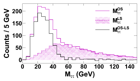
The main challenge in measuring the invariant di-tau mass is the background created by uncorrelated pairs. From the decay chain in question, it is clear that similarly charged ’s are definitely uncorrelated and hence model this background quite well. Thus, we perform the opposite-sign (OS) minus like-sign (LS) subtraction on ’s to obtain the signal.
Figure 1 shows the histogram graph we obtained for the distribution. The luminosity is fb-1, and we can see that a clear end-point is obtained.
III.1.2
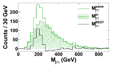
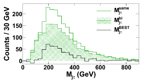
The leptons from each event are sorted into OS and LS pairs. Then, each pair is combined with the leading jets from the same event, and the invariant mass distribution is obtained. At this stage the Bi-Event Subtraction Technique (BEST) Dutta:2011gs is initiated, by first combining the pair with leading jets from a separate event (which we also call a bi-event), to form the distribution . Since jets from a separate event are kinematically uncorrelated with the pair from the current event, this bi-event distribution models the jet background very well.
We note that the greater the number of different-event jets included in the bi-event distribution, the better the modelled background becomes. We include sufficient number of different-event jets to ensure a smooth background distribution.
After this, two subtractions are performed to obtain the final signal: The OSLS subtraction, which gets rid of uncorrelated pairs and The BEST subtraction, which gets rid of uncorrelated jets in the background. In Figure 2, we show the distribution where we find a very clear end point after the BEST subtraction.
III.1.3 Slope of of
The mass of the lies between the two lightest neutralinos, and its exact location approximately determines the of the ’s in the ditau pair. The slope of the visible distribution of the lower energy visible from the di-tau pair (which we will denote by ) is generally a good observable, that carries information about the masses of and (in the case that the lower energy is from ). If the stau mass is very close to the neutralino mass (in the case of stau-neutralino coannihilation) we have a low energy and the slope of the distribution is a good observable.
Conversely, if the visible of a is large, the slope of the distribution is not a good observable. This is because the slope in the case of a higher energy doesn’t show enough variation. In such cases, we use the kinematic information of the high energy by combining it with a leading jet to construct . We will use the endpoint of the distribution as an observable in the stau-neutralino coannihilation case, where one of the ’s has large compared to the other.
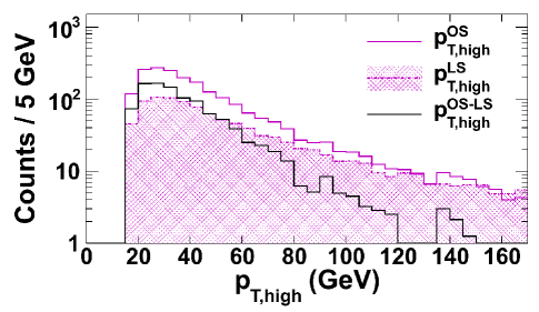
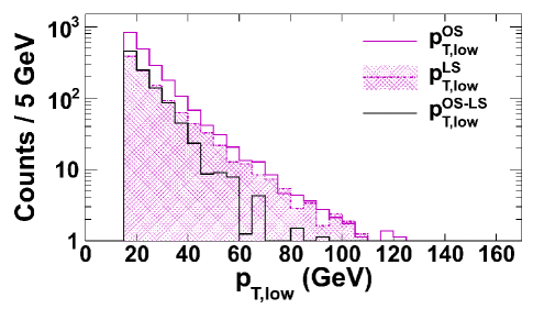
If the stau is somewhat in between the two neutralinos, the slopes of the distributions of both taus become good observables (provided, of course, that neither is too large) as happens in this case. In such a scenario, we get two observables depending on two neutralinos and the stau mass without involving any jet. It is convenient to define the new observables and , which are the arithmetic mean and difference of the slopes of the higher and lower s. These variables can typically be measured down to lower luminosity than , since they do not involve the subtractions required for observables involving jets, as we describe below.
To obtain the distributions, first the OSLS subtraction is performed. Then, we take the logarithm of the and distributions for the higher and lower energy respectively. The histograms are fitted using a linear function to find the slopes. Finally, the slopes are combined into the arithmetic mean and the difference :
| (11) |
Note that these observables, formed by combining the information of the two ’s, are particularly necessary in the case when they are close in mass, since we do not know if a given is originating from the decay or the decay.
III.2 jets +
The distribution is formed by combining the of the first four leading jets and the missing energy
| (12) |
These jets effectively come from the gluino and squark decays.
The effective mass is constructed from the 4jets + sample, with the following cuts
Number of jets: At least four jets in the event;
Leading jet cuts: The first two leading jets each have GeV in ;
Soft jet cuts: Jets with GeV in are accepted in the analysis;
The jets are not tagged;
GeV;
GeV;
No s and s with GeV;
Transverse sphericity .
In Figure 5, we show the distribution at the benchmark point. The peak of this distribution shows a well defined peak for fb-1 luminosity.
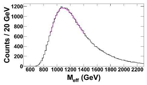
In Table 5, we show the end points of and distributions, peak of the distribution, and the slopes of the distributions for the taus for our benchmark point. The statistical uncertainties range between .
| Observable | Value | fb-1 Stat. | fb-1 Stat. |
|---|---|---|---|
III.3 Observables for the Determination of Third Generation Squark Masses: and
To probe the third generation squark masses we need to involve quarks. The relevant decay chain associated with the dominant production process for the reconstruction of third generation squarks in the stop coannihilation region is
| (13) |
These signals are characterized by high jets accompanied by a and .
We will be constructing the distributions and .
The cuts for the analysis are
GeV;
Number of jets: ;
Leading jet cuts: The first two leading jets each have GeV in . They could be gluon, light-flavor, or jets;
Soft jet cuts: Any jets with visible GeV in are accepted in the analysis. This includes -tagged jets;
GeV;
For , at least one tight jet is required.
The first step in the analysis is the reconstruction of the boson. The appears in the detector as two jets whose invariant mass falls in the mass window ( GeV GeV). We thus choose soft jet pairs (from the third leading jet and below) which are not -tagged, with . The jets are put into two categories: those which are manifestly in the window, and those that fall within the sideband window ( GeV GeV or GeV GeV). BEST is then performed for the two categories, to get rid of uncorrelated jet background. After this, the sideband subtraction is performed to obtain the mass.
Once the is reconstructed, it is paired up with jets to form the and distributions.
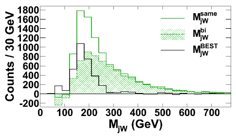
For the distribution, we pair the with a non -tagged soft jet, whose rank is three or lower. This is because we are in the stop coannihilation region. In Figure 6, we show the distribution at the benchmark point, finding a well defined end-point for fb-1 luminosity.
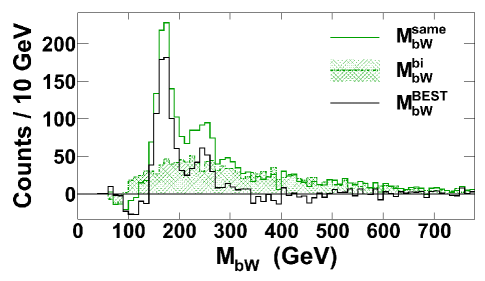
For the distribution, we pair the with a jet of any rank from the current event. Note that the relevant jet required to construct this observable need not be a leading jet; in fact, the leading jet will typically be non -tagged. After pairing the with the jet, we do a further BEST to get rid of uncorrelated jets. This gives the final signal for . However, the signal shows the presence of the unwanted top peak, which comes from . The top window is removed from the final signal, by discarding events with GeV. In Figure 7, we show the distribution obtained at the benchmark point, finding the end-point for fb-1 luminosity.
In Table 6, we show the endpoint values obtained from these distributions. The statistical uncertainties range between . The statistical uncertainty is larger for due to the jet.
| Observable | Value | fb-1 Stat. | fb-1 Stat. |
|---|---|---|---|
IV Determination of Particle Masses, Gaugino Unification Scale, and UV Model Parameters in the Stop Coannihilation Region
The observables measured in Section III are used to determine the masses of the gluino, , , , and , which lead to the determination of model parameters . We will also determine the and masses later in this section.
Theoretically, the functional dependences of the observables in Section III are expected to be:
The masses are varied independently around the benchmark point, and the full simulation of the collider experiment and determination of the observables is performed each time. Thus, the functional dependence of the observables on the masses is determined, along with their uncertainties.
This set of equations can be used to solve for the masses. In general, the dependence of the observables on the masses is expected to be non-linear, corresponding to multiple solutions of the masses. However, near the benchmark point, we found that for most masses, linear functions fitted the dependence quite well. We obtained two solutions only for the stau mass, and one was quite far from the benchmark point and thus rejected. We will have more to say on these issues in Section V.1.
In Table 7, we show the solution to the and masses for fb-1 luminosity. We also show the statistical uncertainties, which range between .
| Particle | Mass | fb-1 Stat. | fb-1 Stat. |
|---|---|---|---|
| 646 | 14,+19 | 11,+14 | |
| 638 | 34,+42 | 23,+39 | |
| 318 | 3,+3 | 3,+3 | |
| 333 | 7,+11 | 6,+8 | |
| 276 | 8,+13 | 7,+10 |
IV.1 Determination of UV Model Parameters and Relic Density
Having determined the masses of and , we can use these to numerically solve for the parameters of the full model. As we have stressed in Section I, the point of this work is to show that the contours of the mediation scheme (here, mirage pattern) show up unmistakably from the determination of certain masses. We will demonstrate this in Section IV.3, where we will show the gaugino unification scale. However, a set of masses may point back at different models, and in particular, we will not attempt to perform a distinguishability study of our particular model. When we solve the model parameters for our particular example (KKLT), our methods will reflect this - we will start from the model parameters, fit with the spectrum, and zero in on the masses we solved.
We use the Nelder Mead method, a commonly used nonlinear optimization technique, to do so. An initial simplex is chosen on the parameter space and ISAJET isajet is used to find the corresponding mass. The scan over parameter space proceeds until the masses calculated by ISAJET are close to the solved values.
Table 8 shows the corresponding model parameters we determined from , , , and for fb-1 and fb-1 luminosities. At fb-1, the statistical uncertainties range between .
| Parameter | Value | fb-1 Stat. | fb-1 Stat. |
|---|---|---|---|
Using the model parameters from Table 8, we calculate the relic density and we find:
| (15) |
The relic density is determined to an accuracy of .
IV.2 Determination of and Masses
The observables and are used to determine the third generation squark masses, once the other masses have been obtained with the observables previously determined.
Theoretically, the functional dependences are and . As before, the masses are varied independently around the benchmark point, and the collider experiment and determination of and is performed each time.
We show the masses of the third generation squarks with uncertainties in Table 9. The statistical uncertainties range between .
| Particle | Mass | fb-1 Stat. | fb-1 Stat. |
|---|---|---|---|
| 531 | 60, +60 | 47, +47 | |
| 326 | 5, +8 | 4, +7 |
IV.3 Gaugino Unification
Upto this point, we have displayed our techniques of reconstructing masses at the benchmark point given in Table 2. Our techniques work perfectly well at benchmark points with higher gluino mass, as preferred by current LHC data. Higher luminosity is of course required to obtain endpoints. Below, we choose such a benchmark point with TeV, reconstruct gaugino masses, and show the gaugino unification scale.
| Parameter | Value | Particle | Mass |
|---|---|---|---|
| 3.8 | 1187 | ||
| 34800 | 740 | ||
| 0.0 | 666 | ||
| 0.5 | 721 | ||
| 28 | 1189 |
For this benchmark point, a luminosity of fb-1 is required to solve for all the masses, following the techniques we have shown in this paper. We show the masses we obtained for this benchmark point in Table 11. The statistical uncertainties range between .
| Particle | Mass | Stat. |
|---|---|---|
| 690 | 6 | |
| 1002 | 126 | |
| 717 | 10 | |
| 1133 |
The model parameters are solved as before, using the masses above as well as the gaugino masses solved at fb-1. The solution to the model parameters at fb-1 for the new benchmark point are and . The relic density is found to be .
As mentioned in Section I, gaugino masses may be obtained at lower luminosity, as we elaborate below.
The solution of gaugino masses typically requires the values of four observables ( and ), as is clear from the solutions we displayed in Table 7. One could have used the endpoint of the invariant mass distribution of the leading jet and the more energetic as an observable. Our analysis of this observable indicates that one requires more luminosity to find its endpoint, relative to the luminosity required to determine the observables and , because of the associated jet subtractions.
Since for the benchmark point the ’s are quite close in mass, we use and , obviating the need to use observables which involve jet information. Then, and masses can be obtained from and observables. Since these observables do not involve jet subtractions, they give acceptable endpoints at lower luminosity. On the other hand, roughly gives the gluino mass.
In Table 12, we show the values of the gaugino masses at fb-1 for the new benchmark point. The statistical uncertainties range between .
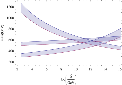
In Figure 8, we show the running of the gauginos and the gaugino unification for our benchmark point. Clearly, gaugino unification occurs below the GUT scale, establishing the footprints of anomaly contributions to supersymmetry breaking.
| Particle | Mass | fb-1 Stat. |
|---|---|---|
| 1181 | 50 | |
| 738 | 15 | |
| 649 | 20 |
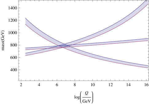
The theoretically expected gaugino unification scale, for this benchmark point, is given by
| (16) |
Note that the expression differs from the ones in Choi:2007ka by the rescaling in Eq. 8.
IV.4 Systematic Errors
We also study an impact due to a uncertainty on the energy scale for jets, taus, and missing transverse energy to estimate the systematic uncertainties independently of luminosity.
Table 13 shows the percentage systematic errors in the determination of the observables and masses. We find that the systematic errors for the observables are between , which is larger than the statistical error at fb-1. The systematic errors of masses, which vary from , are also large compared to the statistical errors, which range between at fb-1. Since our assumption of on the energy scale could be changed in actual experimental conditions, we just show the size of errors in Table 13 as a reference and don’t use them in the analyses performed in the previous sub-sections.
| Observable | Error (%) | Mass | Error (%) | Parameter | Error (%) |
|---|---|---|---|---|---|
| 3.0 | 3.9 | 5.9 | |||
| 4.5 | 2.4,+4.2 | 5.9 | |||
| 5.2 | 4 | 12.5 | |||
| 1.0 | 2.6 | 17 | |||
| 1.3 | 13,+15 | 6.1 | |||
| 5.9 | 2.5,+3.7 | ||||
| 3.7 | 19 |
V Analysis in the Stau Coannihilation Region
In this Section, we determine masses and model parameters for a different point in parameter space, where only stau coannihilation is operational. We first show our analysis for the benchmark model point shown in Table 3. In Section V.3, we will also analyse a benchmark point with heavier gluino mass preferred by current LHC data.
The distributions used in the stau coannihilation region are , , , , and . Note that we only use the corresponding to the lower energy from , since the higher energy doesn’t show enough variation as the masses are varied.
We use , which is formed by combining the higher energy with a leading jet from the same event. OSLS and BEST are performed as usual. Theoretically, one expects .
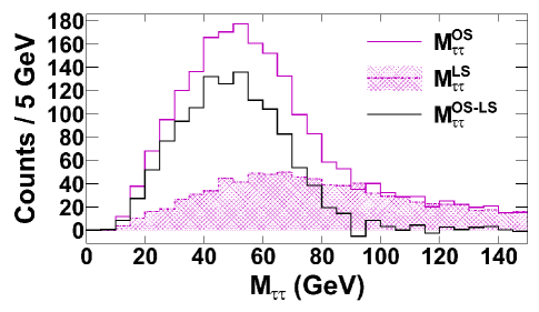
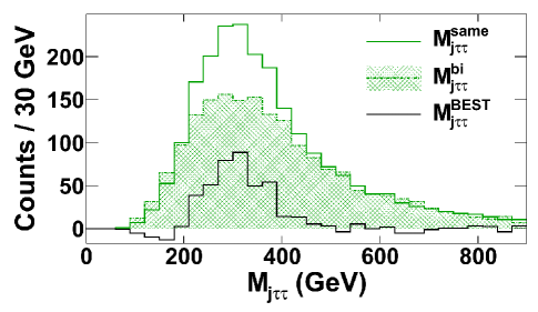
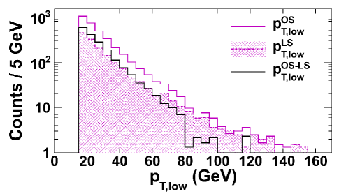
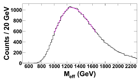
In Table 14, we present the endpoints obtained from the and distributions, the slope of the visible distribution of the lower energy , and the peak of the distribution, at fb-1 for the stau coannihilation benchmark point. The statistical uncertainties range between .
| Observable | Value | fb-1 Stat. |
|---|---|---|
V.1 Masses and Gaugino Unification
After obtaining the values of the observables at the benchmark point as quoted above, we varied the masses around the benchmark point. For each mass selection, we simulated the experiment and obtained all the observables. This gave us the observables as a function of the masses. We then iteratively solved for the masses.
Obviously, one should expect more than one set of mass solutions in this method, since the dependence of the observables on the masses near the benchmark point is non-linear. In this case, we found two sets of solutions with quite disparate values of masses.
This is a general problem, and we mention some arguments to reject the ”wrong” solutions. Firstly, one set of solutions had masses far away from the benchmark point, where the expansion was not performed to begin with. Secondly, this set had a much larger stau-neutralino mass difference, which did not satisfy the relic density constraint.
Finally, one can reject masses by appealing to the UV model and determining more observables, although this goes somewhat against the bottom-up philosophy we have pursued in this paper. Thus, we can use this set of mass solutions and solve for the UV model parameters, which we can then use to solve the spectrum of the model, in particular obtaining the quark mass. Given the spectrum, we can obtain the theoretical value of a particular observable, say , and on the other hand, measure it using the techniques outlined in the paper. For the incorrect mass solution set, the values thus obtained will be very different.
In any case, after rejecting the first set of solutions, the second set itself had two sets of values of and masses, which were close to each other. One set of solutions is shown in Table 15. The other solutions to the and masses are GeV and GeV. All combinations of masses (four in all) are used to solve the model parameters, as we outline in the next subsection.
We display the solution set in Table 15, obtained at luminosity fb-1. The statistical uncertainties are .
| Particle | Mass | fb-1 Stat. |
|---|---|---|
| 895 | ||
| 845 | ||
| 388 | ||
| 298 | ||
| 274 |
V.2 Determination of UV Model Parameters and Relic Density
Having determined the masses of , and , we can use these to numerically solve for the parameters of the full model.
We use the Nelder-Mead method to do so. An initial simplex is chosen on the parameter space and ISAJET is used to find the corresponding mass. The scan over parameter space proceeds until the masses calculated by ISAJET are close to the solved values.
In the previous subsection, we have discussed two solutions each for and . We solved the model parameters for each combination of masses (four in all), and took the average of the values of the model parameters thus obtained. These average values are displayed in Table 16. The statistical uncertainties are .
| Parameter | Value | Stat. |
|---|---|---|
| 7.42 | 0.58 | |
| 10171 | 882 | |
| 0.52 | 0.09 | |
| 1.17 | ||
| 33.1 | 7.8 |
Using the model parameters from Table 16, we calculate the relic density and we find:
| (17) |
The relic density is thus determined to an accuracy of .
V.3 Gaugino Unification
Although upto this point, we have displayed our results in the stau coannihilation region at the benchmark point given in Table 4, our methods are applicable at other benchmark points with higher gluino mass, preferred by current LHC data. We display such a benchmark point for stau coannihilation below, and proceed to show gaugino unification.
| Parameter | Value | Particle | Mass |
|---|---|---|---|
| 10 | 1183 | ||
| 9500 | 499 | ||
| 0.5 | 337 | ||
| 1.0 | 361 | ||
| 37 | 1119 |
At this benchmark point, we found acceptable endpoints at fb-1, and solved for the observables and masses. The masses are GeV and GeV. The masses of the gauginos can also be determined, although we show their values at a lower luminosity below. After determining the masses, the observables can be solved and they are and . The relic density for the heavy gluino point is found to be .
The gaugino masses can be obtained at lower luminosity, as spelled out in Section I.
In the stau coannihilation region, one can use the proximity of the stau and lightest neutralino masses to solve gaugino masses using fewer observables, in particular avoiding the observable , which typically requires higher luminosity due to jet subtractions. This is reminiscent of what we did in the previous sections with stop coannihilation, although there we used the proximity of ’s.
We take approximately
| (18) |
Thus, assuming that is approximately determined by , it is clear from Eq. IV that one can solve for from and .
These observables have acceptable endpoints and peaks down to fb-1. The main difference from the full set of observables is the distribution, which requires a higher luminosity to obtain acceptable endpoints due to jet subtractions.
In Table 18, we show the gaugino masses obtained at fb-1 for the new stau coannihilation benchmark point with heavier gluino. The statistical uncertainties are .
| Particle | Mass | fb-1 Stat. |
|---|---|---|
| 1186 | 84 | |
| 527 | ||
| 317 | 33 |
In Figure 14, we show gaugino unification for the new benchmark point at fb-1.
VI Conclusions
If supersymmetry is discovered at the LHC, the next step would be to understand as much as possible about the underlying model of supersymmetry breaking and mediation. How should one proceed?
One option is to start from specific models defined by a tractable number of parameters at high energy, and fit to observables measured in the collider. However, we have stressed that a given set of measured observables will generally point back at different UV models, distinguishing among which may be challenging and even intractable (depending on the complexity of the model and the number of reliable observables measured).
We have stressed on a bottom-up approach to this question: first identify sectors in the low energy spectrum which carry the imprints of mediation schemes in a relatively model-independent manner, next construct observables which carry information about these masses, and finally using the observables solve for the masses and identify a mediation scheme.
The gaugino sector offers a particularly fruitful sector in this program, since the determination of this sector can unambiguously show the imprints of anomaly contributions to supersymmetry breaking. We therefore take an example of a model where anomaly contributions are significant (supersymmetry breaking in KKLT compactification) and proceed to obtain the gaugino masses, by constructing suitable observables.
We rely on the construction of kinematic observables arising from cascade decays using endpoint techniques, since these are a particularly sharp tool for such diagnosis.
While the gauginos are important in the paradigm outlined above, they form only a subset of the masses we determined in this paper. Given a neutralino dark matter, the determination of other masses becomes a necessity when one wants to establish mechanisms to satisfy the relic density. This is perfectly amenable to the kind of bottom-up approach we have taken: in our examples, we needed to establish that the stop-neutralino and stau-neutralino coannihilation mechanisms were operational. To do so demanded the determination of stop and stau masses, in addition to the neutralino.
We summarize our work below:
We constructed observables using different combinations of the jets, ’s and ’s in the final states. We constructed these observables in the stop-neutralino and stau-neutralino coannihilation regions.
In the stop coannihilation region, we constructed two new observables, and , to determine the masses of the and the . The determination of the and masses is especially challenging, since both decay to quarks. To make the problem worse, stop decays to missing energy by emitting a low energy jet in this coannihilation region. We showed how to reconstruct the stop mass in order to establish the fact that we are in the stop-neutralino coannihilation region.
We also constructed two other new observables, and which are combinations of the of two opposite sign ’s. These observables are particularly useful when the sample shows the presence of two opposite sign ’s that are close in mass.
Using the observables, we solved for the masses of the gluino, the two lighter neutralinos, squarks (of the first two generations) and the lightest stau. We also determined the lighter stop and sbottom masses in the stop coannihilation region.
We used the neutralino and gluino masses to determine the gaugino unification scale and discern the effects of anomaly mediation from a bottom-up approach, as elaborated above.
Using all the masses, we determined (a) the model parameters and (b) tested whether we are in a coanihilation region and dark matter relic density is satisfied. We find that relic density can be determined with an accuracy of in the stop and in the stau coannihilation region.
As far as the diagnosis of the supersymmetry breaking mediation scheme is concerned, the most important future direction is obviously to expand our techniques to parts of the parameter space away from the coannihilation regions. Our observables enabled us to solve for the lightest neutralinos, and for the statements on mediation scheme that we made above, they were assumed to be gauginos (this is guaranteed in the coannhilation regions). It would be very interesting to test the paradigm outlined in this paper at regions where the Higgsino component is not insignificant. Also interesting would be to find bottom-up techniques to further distinguish between different schemes that correspond to the same gaugino mass pattern. We leave these questions for future work.
VII Acknowledgements
We would like to thank John Conley and Jamie Tattersall for discussions and Nathan Krislock for introducing us to the Nelder Mead method. K.W. would like to thank Lingzhi Wang for help with programming. T.K. would like to thank D.H. Kim and Y. Oh for their constructive discussions throughout this work. This work is supported in part by the DOE grant DE-FG02-95ER40917 and by the World Class University (WCU) project through the National Research Foundation (NRF) of Korea funded by the Ministry of Education, Science & Technology (grant No. R32-2008-000-20001-0).
References
- (1) S. P. Martin, “A Supersymmetry primer,” In *Kane, G.L. (ed.): Perspectives on supersymmetry* 1-98. [hep-ph/9709356]; H. P. Nilles, “Supersymmetry, Supergravity and Particle Physics,” Phys. Rept. 110, 1-162 (1984).
- (2) J. A. Conley, H. K. Dreiner, L. Glaser, M. Kramer and J. Tattersall, “Using rates to measure mixed modulus-anomaly mediated supersymmetry breaking at the LHC,” arXiv:1110.1287 [hep-ph]. H. K. Dreiner, M. Kramer, J. M. Lindert and B. O’Leary, “SUSY parameter determination at the LHC using cross sections and kinematic edges,” JHEP 1004, 109 (2010) [arXiv:1003.2648 [hep-ph]]. P. Bechtle, K. Desch, M. Uhlenbrock and P. Wienemann, “Constraining SUSY models with Fittino using measurements before, with and beyond the LHC,” Eur. Phys. J. C 66, 215 (2010) [arXiv:0907.2589 [hep-ph]]. C. G. Lester, M. A. Parker and M. J. . White, “Determining SUSY model parameters and masses at the LHC using cross-sections, kinematic edges and other observables,” JHEP 0601, 080 (2006) [arXiv:hep-ph/0508143].
- (3) A. H. Chamseddine, R. L. Arnowitt, P. Nath, Phys. Rev. Lett. 49, 970 (1982); R. Barbieri, S. Ferrara, C. A. Savoy, Phys. Lett. B119, 343 (1982); L. J. Hall, J. D. Lykken, S. Weinberg, Phys. Rev. D27, 2359-2378 (1983); P. Nath, R. L. Arnowitt, A. H. Chamseddine, Nucl. Phys. B227, 121 (1983); For a review, see H. P. Nilles, Phys. Rept. 110, 1-162 (1984).
- (4) G. F. Giudice, R. Rattazzi, “Theories with gauge mediated supersymmetry breaking,” Phys. Rept. 322, 419-499 (1999). [hep-ph/9801271]. L. Randall, R. Sundrum, “Out of this world supersymmetry breaking,” Nucl. Phys. B557, 79-118 (1999). [hep-th/9810155]; G. F. Giudice, M. A. Luty, H. Murayama, R. Rattazzi, “Gaugino mass without singlets,” JHEP 9812, 027 (1998). [hep-ph/9810442].
- (5) J. P. Conlon, F. Quevedo and K. Suruliz, “Large-volume flux compactifications: Moduli spectrum and D3/D7 soft supersymmetry breaking,” JHEP 0508, 007 (2005) [hep-th/0505076].
- (6) K. Choi, K. S. Jeong, K. -i. Okumura, “Phenomenology of mixed modulus-anomaly mediation in fluxed string compactifications and brane models,” JHEP 0509, 039 (2005). [hep-ph/0504037].
- (7) S. Kachru, R. Kallosh, A. D. Linde and S. P. Trivedi, “De Sitter vacua in string theory,” Phys. Rev. D 68, 046005 (2003) [arXiv:hep-th/0301240].
- (8) K. Choi and H. P. Nilles, “The gaugino code,” JHEP 0704, 006 (2007) [arXiv:hep-ph/0702146].
- (9) D. E. Kaplan, G. D. Kribs and M. Schmaltz,“Supersymmetry breaking through transparent extra dimensions,” Phys. Rev. D 62, 035010 (2000) [hep-ph/9911293]. Z. Chacko, M. A. Luty, A. E. Nelson and E. Ponton, “Gaugino mediated supersymmetry breaking,” JHEP 0001, 003 (2000) [hep-ph/9911323]. M. Schmaltz and W. Skiba, “Minimal gaugino mediation,” Phys. Rev. D 62, 095005 (2000) [hep-ph/0001172].
- (10) R. L. Arnowitt, B. Dutta, A. Gurrola, T. Kamon, A. Krislock and D. Toback, “Determining the Dark Matter Relic Density in the mSUGRA Stau-Neutralino Co-Annhiliation Region at the LHC,” Phys. Rev. Lett. 100, 231802 (2008) [arXiv:0802.2968 [hep-ph]].
- (11) I. Hinchliffe, F. E. Paige, M. D. Shapiro, J. Soderqvist and W. Yao, “Precision SUSY measurements at CERN LHC,” Phys. Rev. D 55, 5520 (1997) [arXiv:hep-ph/9610544]. I. Hinchliffe and F. E. Paige, “Measurements in SUGRA models with large tan(beta) at LHC,” Phys. Rev. D 61, 095011 (2000) [arXiv:hep-ph/9907519].
- (12) B. C. Allanach and M. J. Dolan, “Supersymmetry With Prejudice: Fitting the Wrong Model to LHC Data,” arXiv:1107.2856 [hep-ph].
- (13) B. Dutta, T. Kamon, A. Krislock, N. Kolev and Y. Oh, “Determination of Non-Universal Supergravity Models at the Large Hadron Collider,” Phys. Rev. D 82, 115009 (2010) [arXiv:1008.3380 [hep-ph]].
- (14) R. Rattazzi, A. Strumia and J. D. Wells, “Phenomenology of deflected anomaly mediation,” Nucl. Phys. B 576, 3 (2000) [hep-ph/9912390].
- (15) K. Choi, K. Y. Lee, Y. Shimizu, Y. G. Kim, K. -i. Okumura, “Neutralino dark matter in mirage mediation,” JCAP 0612, 017 (2006). [hep-ph/0609132]. H. Baer, E. -K. Park, X. Tata, T. T. Wang, “Collider and Dark Matter Phenomenology of Models with Mirage Unification,” JHEP 0706, 033 (2007). [hep-ph/0703024].
- (16) P. Gondolo, J. Edsjo, P. Ullio, L. Bergstrom, M. Schelke, E. A. Baltz, “Darksusy - a numerical package for supersymmetric dark matter calculations,” [astro-ph/0211238].
- (17) F. E. Paige, S. D. Protopopescu, H. Baer and X. Tata, “ISAJET 7.69: A Monte Carlo event generator for p p, anti-p p, and e+ e- reactions,” [hep-ph/0312045]. We use ISAJETversion 7.74.
- (18) T. Sjostrand, S. Mrenna, and P. Skands, ”PYTHIA 6.4 Physics and Manual.” J. High Energy Phys. 05 (2006) 026. We use PYTHIA version 6.411 with TAUOLA.
- (19) PGS4 is a parameterized detector simulator. We use version 4 (http://www.physics.ucdavis.edu/~conway/research/software/pgs/pgs4-general.htm) in the CMS detector configuration. We assume the identification efficiency with GeV is 50%, while the probability for a jet being mis-identified as a is 1%. The -jet tagging efficiency in PGS is 42% for 50 GeV and , and degrading between . The -tagging fake rate for and light quarks/gluons is and , respectively.
- (20) CMS Collaboration, ”Search for Physics Beyond the Standard Model in Events with Opposite-sign Tau Pairs and Missing Energy”, CMS Physics Analysis Summary CMS-PAS-SUS-11-007 (2011).
- (21) B. Dutta, T. Kamon, N. Kolev and A. Krislock, “Bi-Event Subtraction Technique at Hadron Colliders,” Phys. Lett. B 703, 475 (2011) [arXiv:1104.2508 [hep-ph]].