An estimate of the temporal fraction of cloud cover at San Pedro Mártir Observatory

Abstract

San Pedro Mártir in the Northwest of Mexico is the site of the Observatorio Astronómico Nacional. It was one of the five candidates sites for the Thirty Meter Telescope, whose site-testing team spent four years measuring the atmospheric properties on site with a very complete array of instrumentation. Using the public database created by this team, we apply a novel method to solar radiation data to estimate the daytime fraction of time when the sky is clear of clouds. We analyse the diurnal, seasonal and annual cycles of cloud cover. We find that 82.4 per cent of the time the sky is clear of clouds. Our results are consistent with those obtained by other authors, using different methods, adding support to this value and proving the potential of the applied method. The clear conditions at the site are particularly good showing that San Pedro Mártir is an excellent site for optical and infrared observations.

1 Introduction

The San Pedro Mártir (SPM) observatory is located at $31^{\circ}02^{\prime}39^{\prime\prime}$N, $115^{\circ}27^{\prime}49^{\prime\prime}$W and at an altitude of 2830 m, inside the Parque Nacional Sierra de San Pedro Mártir. SPM is $\sim$65 km E of the Pacific Coast and $\sim$55 km W to the Gulf of California. The largest telescope at the site is a 2.1-m Ritchey-Chrétien, operational since 1981. Astroclimatological characterization studies at SPM are reviewed in Tapia, Hiriart & Cruz-González (2007). Compilations of one and two continuous decades of weather and observing statistics of OAN-SPM have been reported by  Tapia (1992) and  Tapia (2003). The yearly fractions of photometric and spectroscopic nights from 1984 to 2006 is presented on Table 3 of Tapia, Hiriart & Cruz-González (2007). Other aspects of the site characterization have been reported by several authors e.g. Cruz-González et al. (2003) and Cruz-González, et al. (2007). Nevertheless, this is the first study on the radiation data measured in situ. The data were recorded by the Thirty Meter Telescope (TMT) site-testing team from 2004 to 2008; see Schöck et al. (2009) for an overview of the TMT project and its main results.

Cloud cover is one of the most important considerations to characterize a ground-based astronomical observatory. Only for low-frequency radio observations cloudiness is of little importance. Given a site, statistics of daytime cloud cover are indicative of the usable portion of the time for optical and near-infrared observations and bring key information for the potentiality of that site for millimeter and sub-millimeter astronomy. The relationship between diurnal and nocturnal cloudiness is strongly dependent on the location of the site. Erasmus & Van Staden (2002) give a detailed discussion on that topic. For the case of SPM these authors conclude that the day versus night variation of the cloud cover is less than 5 per cent. Therefore, daytime cloud cover statistics at SPM is a useful indicator of nighttime cloud conditions. Here we present a study of the cloud cover over SPM using an approach recently introduced by Carrasco et al. (2009). It consists of the computation of histograms of solar radiation values measured at the site and corrected for the zenital angle of the Sun. The data coverage is presented in section §2, the method is described in §3, the data obtained in SMP §4, the discussion of the results in §5, the statistics of cloud cover in §6 and the summary and conclusions in §7.

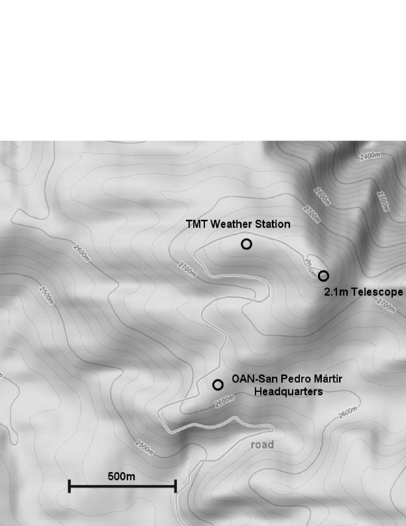
Figure 1: Location of the TMT automatic weather station relative to the the 2m telescope and the observatory headquarters. The 2.1m telescope is at 31.04417^∘N, 115.463611^∘W.

2 Data coverage

The data presented here consist of records of solar radiation energy fluxes in units of Wm^-2 acquired with an Monitor automatic weather station (Schöck et al., 2009), located 2m above the ground (Skidmore et al., 2009) at 31^∘ 02${}^{{}^{\prime}}$ 43.84^" N, 115^∘ 28${}^{{}^{\prime}}$ 10.45^" W. It was in a tree free zone without visibility limitations. The location of the weather station relative to the observatory headquarters is shown in Fig. 1. The Monitor sensors have a spectral response between 400 and 950 nm with an accuracy of 5 per cent according to the vendor. The data span between October 2, 2004 and August 8, 2008 with a sampling time of 2 minutes.

The analysis does not include the data from 2004, when the radiation sensor was not working at the beginning of each day. Table 1 summarises the temporal coverage of the data expressed in percentage, with due considerations of the diurnal cycle variation. The data span from 2005 January 12 to 2008 August 8, with a 67 per cent effective coverage of the 3.6 year sample; data exist for 973 out of 1316 days. The complete sample contains 596580 min out of 899520 possible; coverage was 59 per cent for 2005 and increased to 78 per cent towards the end of the campaign, in 2008. In Fig. 2 the solid line shows the total number of hours per month of solar radiation measured in situ while the red dotted line represents the corresponding expected radiation flux. The coverage per hour of day, shown in Table 2, was obtained by counting the minutes of data and comparing with the total expected, given SPM coordinates. Hours with very low data coverage, less than 30 min, are excluded in this analysis.

Table 1: Solar radiation data coverage in percentage.

Month	2005	2006	2007	2008	All
January	63	74	60	33	57
February	93	92	86	92	91
March	73	22	63	85	61
April	68	0	45	94	52
May	69	34	100	96	75
June	69	94	59	97	80
July	66	81	99	96	86
August	0	81	96	24	50
September	0	95	0	-	32
October	83	97	72	-	84
November	91	79	78	-	83
December	44	39	44	-	42
Year Total	59	65	68	78	67

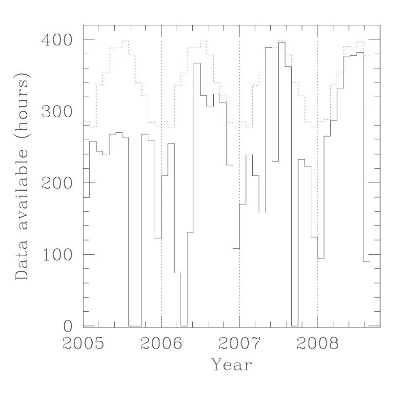
Figure 2: Data coverage in hours per month. The red dotted lines are the hours of solar radiation at the site per month for the same period.

Table 2: Hourly solar radiation data coverage in percentage.

	Jan	Feb	Mar	Apr	May	Jun	Jul	Aug	Sep	Oct	Nov	Dec	Per hr
6 h	-	-	-	25	77	75	100	0	0	-	-	-	69
7 h	-	-	49	37	56	62	74	52	35	99	-	-	54
8 h	80	100	51	37	56	62	75	52	32	82	88	-	68
9 h	62	100	52	37	56	61	75	52	32	84	92	57	63
10 h	61	99	70	58	80	86	91	52	32	84	90	43	71
11 h	49	94	71	59	81	86	91	52	32	78	57	26	66
12 h	48	97	71	59	80	88	91	50	32	85	90	30	69
13 h	61	97	68	58	80	88	91	50	32	83	91	46	71
14 h	60	94	66	58	80	88	90	51	32	83	92	46	71
15 h	60	93	65	58	80	88	91	51	32	81	93	46	70
16 h	50	87	65	58	78	88	90	51	29	82	92	47	68
17 h	30	47	46	56	79	91	89	51	31	97	-	-	57
18 h	-	-	-	57	93	88	90	55	24	-	-	-	71
Per month	57	91	61	52	75	81	87	50	32	84	83	42	67

3 Solar radiation and inferred cloud coverage

In this section we present the model used to retrieve the cloud coverage from the radiation data developed by Carrasco et al. (2009) for Sierra Negra, the site of the Large Millimeter Telescope (LMT) and the High Altitude Water Čerenkov $\gamma$-ray observatory (HAWC).

The radiation flux at ground level is considered, to first approximation, to be given by the solar constant $F_{\sun}$, modulated by the zenith angle of the Sun and a time variable attenuation factor $\psi(t)$. For working purposes we take $F_{\sun}=1367\,\rm Wm^{-2}$ exactly. The solar constant varies only $\pm 1$ Wm^-2 over the 11 yr solar cycle, (1998). These variations are negligible for the purpose of this work. Knowing the position of the Sun at the site as a function of time, we can estimate the variable $\psi$, given as

$$\psi(t)={F(t)\over F_{\sun}\cos\theta_{\sun}}\,.$$ (1)

where $F(t)$ is the radiation measured at the site and $\theta_{\sun}$ is the zenith angle of the Sun. $\psi(t)$ is a time variable factor, nominally below unity, which accounts for the instrumental response (presumed constant), the atmospheric extinction on site and the effects of the cloud coverage. Knowing the site coordinates, we compute the modulation factor $\cos\theta_{\sun}$ as a function of day and local time, minute per minute to study the behavior of the variable $\psi$. In the case of Sierra Negra the histogram of values of $\psi$ showed a clear bimodal distribution composed by a broad component for low values of $\psi$ and a narrow peak $\psi\la 1$. The histogram of $\psi$ values (Fig. 11 of Carrasco et al., 2009) can be well reproduced with a two component fit, with the first component having its maximum around $\psi\sim 0.2$ and the narrow peak at $\psi\sim 0.75$, with the minimum at $\psi_{min}=0.55$ separating both components. The narrow component is interpreted as due to direct sunshine while the broad component is originated when solar radiation is partially absorbed by clouds; we then use the relative ratio of these two components to quantify the “clear weather fraction”.

The functional form of the fit to the histogram of $\psi$ is given by,

$$f(\psi)=A\psi^{2}e^{-\beta\psi}+{B\over 1+\left[(\psi-\psi_{0})/\Delta\psi\right]^{2}}.$$ (2)

The first term on the right hand side is a $\chi^{2}$ function with six degrees of freedom. It is interpreted as the “cloud-cover” part of the data, with its integral being the fraction of “cloud-covered” time. The second term, a Lorentzian function with centre $\psi_{0}$ and width $\Delta\psi$, represents the “cloud-clear” part of the data. $A$ and $B$ provide the normalization and relative weights of both components; $\beta$ is related to the width and centre of the broad peak.

4 San Pedro Mártir data

Daily minute per minute values of the atmosphere free modulated solar radiation flux, $F_{\sun}\cos\theta_{\sun}$, were compared with the radiation measured at the site. Local transit cosine values range just below 1 around June 16 and July 1 (for 2005) to 0.58 at winter solstice (December 21).

For the analysis described in this section we considered data with airmass below 2 as most astronomical observations are carry out at this airmass interval. The normalized histogram of $\psi$ for all the data is shown in the upper panel of Fig. 3. It shows a double peak in the clear component, not fully consistent with the standard narrow component fit function, and the cloud component with maximum at $\psi\la 0.3$. We applied the double component fit of Eq. 2, shown in the lower panel of Fig. 3. The fit for the clear component is drawn in blue, for the cloud component in green and for the sum in red. The coefficients of the fit given by Eq. 2 are presented in Table 3. Fit errors were obtained through a bootstrap analysis using 10000 samples. The fit agrees with the data within the statistics, except in the wings of the clear peak in Fig. 3. Still, the Lorentzian function proved to fit much better the data than a Gaussian. The fit can be better appreciated in a logarithm version of Fig. 3, shown in Fig. 4.

Table 3: Parameters of the fit shown in red Fig. 3.

Parameter	Global	Bootstrap	errors	relative
	$z<2$			error $(10^{-3}$)
$A$	40.8	40.766	$\pm 0.612$	15.0
$\beta$	7.19	7.175	$\pm 0.044$	6.2
$B$	6.03	6.035	$\pm 0.055$	9.1
$\psi_{0}$	0.815	0.8151	$\pm 0.0002$	0.3
$\Delta\psi$	0.063	0.0629	$\pm 0.0005$	7.5
f(clear)	0.824	0.8238	$\pm 0.0009$	1.1
f(cloud)	0.176	0.1762	$\pm 0.0009$	5.0

We considered data with $\psi\leq\psi_{min}$, where $\psi_{min}=0.58$, as cloudy weather and data with $\psi>\psi_{min}$ as clear weather. The value $\psi_{min}=0.58$ corresponds to the intersection of the two components of the function fitted to the distribution of all data points. We computed the fraction of clear time f(clear), as clear/(clear+cloudy). From the global histogram we obtained a clear fraction for the site of 82.4 per cent. The errors in the determination of f(clear) and f(cloud), were also obtained by generating 10000 bootstrap samples; they are shown in Table 3.

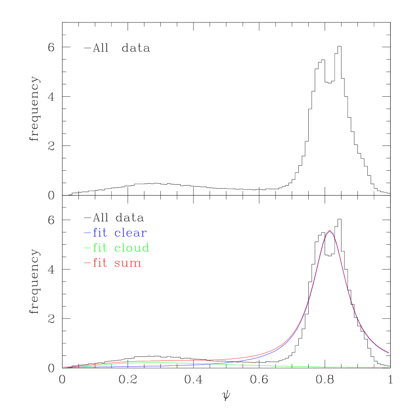
Figure 3: The normalized observed distribution of $\psi$: the solar flux $F(t)$ divided by the nominal solar flux at the top of the atmosphere, $F_{\sun}\cos\theta_{\sun}(t)$ for airmasses below 2. Top: the distribution for all the data. Bottom: the fit to the data is the sum of two components: the blue line corresponds to clear weather; the green one to cloudy weather and the red line to the sum. The relative area of both components determines the clear/cloud fraction. See the electronic edition of MNRAS for a color version of this figure.

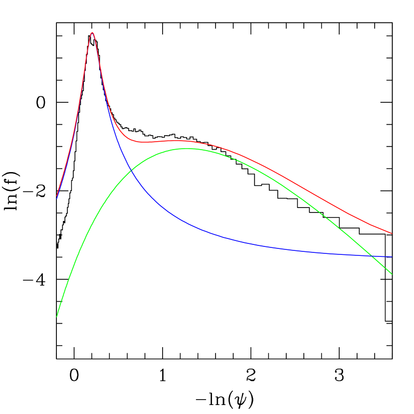
Figure 4: The logarithm plot of the normalized observed distribution of $\psi$ shown in Fig. 3. The blue line corresponds to clear weather; the green one to cloudy weather and the red line to the sum. See the electronic edition of MNRAS for a color version of this figure.

To study the seasonal variation of $\psi$ we created histograms and the corresponding fits per month. Consider the histogram and corresponding fit for July and November shown Fig. 5. It can be appreciated that the fits reproduce the distribution of $\psi$ very well. The narrow clear component is consistent with prevailing clear sky conditions, for which the solar radiation reaches the site with only the attenuation of the atmosphere. The coefficients of the fits presented in Fig. 5, according to the functional form of $f(\psi)$ given by Eq. 2, are shown in Table 4. The fits can be better valued in the logarithm displays of Fig. 5, presented in Figs. 6 and 7. The fits to the complete data (red line), to clear weather (blue line) and to cloudy weather (green line), have been included.

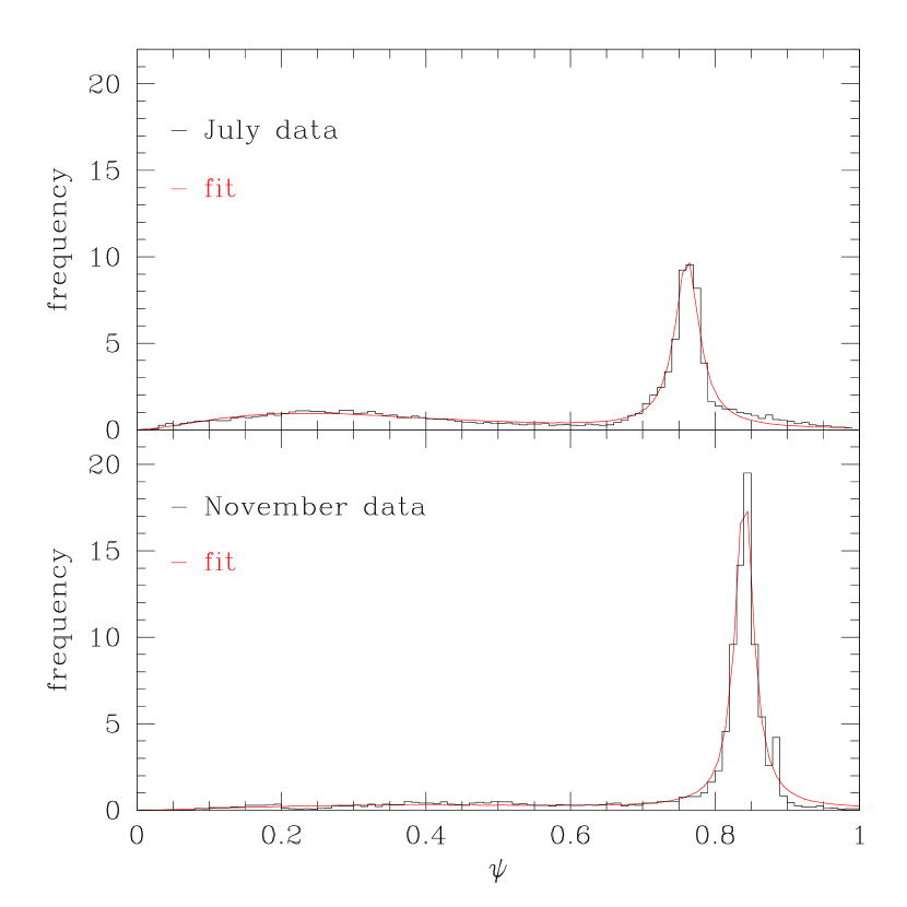
Figure 5: The observed distribution of $\psi$ and the two component fit for July (top) and November (bottom). Comparing both plots a shift in the centre of the narrow component can be appreciated. $\psi$. See the electronic edition of MNRAS for a color version of this figure.

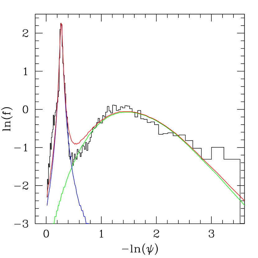
Figure 6: The logarithm plot of the observed distribution of $\psi$ for July shown in the top panel of Fig. 5. The fit to the data is the sum of two components:the blue line corresponds to clear weather; the green one to cloudy weather and the red line to the sum. See the electronic edition of MNRAS for a color version of this figure.

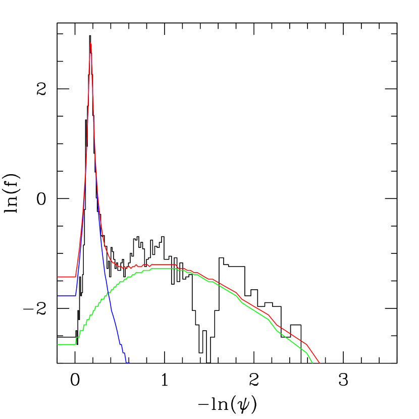
Figure 7: The logarithm plot of the observed distribution of $\psi$ for November shown in the bottom panel of Fig. 5. The fit to the data is the sum of two components:the blue line corresponds to clear weather; the green one to cloudy weather and the red line to the sum. Note that even in the case of low statistics the fit proves to be good. See the electronic edition of MNRAS for a color version of this figure.

Figure 8: The centre of the narrow component of $\psi$ for each month. The monthly values for all the data are indicated by the histogram, while the dots mark individual months of different years. The position of the narrow peak component is not constant during the year, reaching a minimum in July. The error bars are smaller than the symbols.

Table 4: Coefficients of the fits shown in Fig. 5.

Sample	A	$\beta$	B	$\psi_{0}$	$\Delta\psi$
July	135.2	8.68	9.24	0.761	0.021
	$\pm 1.5$	$\pm 0.112$	$\pm 0.141$	$\pm 0.0005$	$\pm 0.001$
November	11.7	3.83	19.07	0.841	0.015
	$\pm 2.6$	$\pm 0.189$	$\pm 0.236$	$\pm 0.0009$	$\pm 0.002$

When analysing the fits per month we realised that the Lorentzian fits for the ”clear weather peak” are better than that of the complete dataset. Futhermore, we noted a significant shift in the position of its centre, that can be clearly appreciated in Fig. 5 where we present the plots for July and November. This effect is also apparent in Figs. 6 and 7.

We studied the position of the centre of the peak corresponding to the clear fraction as a function of the month of each observed year. We found that for every year there is a cyclic effect: the centre of the peak is 0.880 in January, reaches a maximum around 0.889 in February, decreases to a minimum of 0.761 in July and increases towards the end of the year to 0.885 in December. Errors in the statistical determination of $\psi_{0}$ are $\la 0.001$. Fig. 8 shows the position of the centre of the narrow component obtained using the whole data set for each month with a solid line. The corresponding values of the individual months for different years are indicated by distinct symbols.

The solar radiation sensor accuracy is $\pm 5\%$. However, considering N ($\sim$20000) data points per bin, the position of the peaks are statistical variables determined with an accuracy $\propto 1/\sqrt{N}$ times the individual measurement error i.e. much better than 5%. Hence, the variations in the position of the centres observed with an amplitude of up to 14% are statistically robust. Still, the amount of radiation corresponding to the clear peak in July is higher by 277 Wm^-2 than that received in November.

5 Discussion

5.1 Global clear time determination

The 82.4 per cent of clear fraction obtained from the global distribution shown is Fig. 3 is similar to that reported by Erasmus & Van Staden (2002). In a comprehensive study for the California Extremely Large Telescope (CELT) project, the authors surveyed cloud cover and water vapor conditions for different sites using observations from the International Satellite Cloud Climatology Project. The study covers 58 months between July 1993 and December 1999 using a methodology that had been tested and successfully applied in previous studies. They estimated that the photometric and usable fractions of nighttime at SPM are 74 and 81 per cent, respectively. Their definition of usable time includes conditions with high cirrus. The authors give a detailed discussion on the relationship between diurnal and nocturnal cloudiness. For the case of SPM, they conclude that the day versus night variation of cloud cover is less than 5 per cent, being clearer at night.

Another estimation of the useful observing time at SPM is given by  Tapia (2003) who reports a 20 yr statistics of the fractional number of nights with totally clear, partially clear and mostly cloudy based in the observing log file of the 2.1m telescope night assistants. The author reports a total fraction of useful observing time of 80.8 per cent and compares his results with those from  Erasmus & Van Staden (2002); he concludes that the monthly results from both studies agree within 5 per cent while for the yearly fraction, the discrepancies are lower than 2.5 per cent.

5.1.1 The diurnal cycle

Erasmus & Van Staden (2002) studied the diurnal cycle by calculating the average of clear time for two sets of hours: from 8-12 (D1) and from 12-16 (D2), considering data at airmass less than 2 and defining the seasons as follows: winter: December, January and February; spring: March, April and May; summer: June, July and August and autumn: September, October and November. Our results for D1 and D2, using the same parameters, and theirs are shown in Table 5. As we are not comparing simultaneous observations we do not expect to obtain necessarily the same values of clear time for D1 & D2. Nevertheless, we reproduce the differences between them within a few percentage, the largest difference being 7 per cent for winter. The trend in our results for daytime is consistent with that obtained by  Erasmus & Van Staden (2002).

The differences in the values for D1 and D2 and those obtained by  Erasmus & Van Staden (2002) are between 3 and 28 per cent. As a reference, in the case of the PWV, the results for the TMT preliminary studies carried out by  Erasmus & Van Staden (2002) and those obtained from the in situ site testing group are within 30 per cent for all the sites, see Otárola et al. (2010). Our results for D1 & D2 are within that range. Futhermore, the differences might be influenced by the distinct data coverage and by the definitions of clear time used by  Erasmus & Van Staden (2002). The results presented in this paper are based on direct solar radiation measurements.

5.2 The seasonal variation of $\psi_{0}$

Table 5: Percentage of time that sky conditions are clear for two different periods of day D1 & D2.

f(clear)	D1	D2	D1-D2	D1	D2	D1-D2
	This paper			E & VS
Summer	78	66	12	75	60	15
Autumn	88	84	4	70	66	4
Winter	80	83	-3	52	62	-10
Spring	95	94	1	77	75	2

The variation trend in the centre of the clear peak shown in Fig. 8 can be interpreted in terms of seasonal variations of the atmospheric transmission: during the summer months there is more atmospheric absorption than in the rest of the year. This is consistent with the seasonal variation of the Precipitable Water Vapor (PWV) at 210 GHz reported by  Hiriart et al. (1997),  Hiriart et al. (2003),  Otárola et al. (2009, 2010). The seasonal variation in the PWV is shown in Figs. 9, 10 and 11 of  Otárola et al. (2009), where the maximum PWV values occur during the Summer. On the other hand,  Araiza & Cruz-González (2011) showed that the aerosol optical depth has a seasonal variation being higher at spring (maximum) and summer than in the rest of the year (c.f. their Figs. 1, 2, 3 and Table 3). These results suggest that the double peak in the global distribution of $\psi$ is due to absorption variations in the atmosphere.

The larger value of the centres of the clear peak for July 2006 and August 2008 relative to the same months of the other years, shown in Fig. 8, suggest that the atmosphere was more transparent. We analysed the aerosol optical thickness reported by  Araiza & Cruz-González (2011) (c.f. Table 4). The larger value of the centre for July 2006 is consistent with smaller values of the aerosol optical thickness for July 2005 and 2007 but marginally for July 2008. The bigger value of the centre for August 2008 is also consistent with smaller values of the aerosol optical depth for August 2007 and marginally for August 2006 while for August 2005 there is not data available.

6 Statistics of clear time

The solar radiation data observed at airmass lower than 2 is a subset of that observed below 10. For completeness, in this analysis we considered data with airmass less than 10. The fraction of clear time f(clear) was computed for every hour of data, accumulating 7828 h. Fig. 9 shows the distribution of hourly clear fraction. We note that it behaves in a rather unimodal fashion: 78.6 per cent have $f({\rm clear})=1$ while 9.5 per cent of the hours have $f({\rm clear})=0$. The remaining fraction of data (12.5%) have intermediate values.

The contrast between summer and the other seasons is well illustrated in Fig. 10, showing the median and quartile fractions of clear time for successive years. The bars represent the dispersion in the data measured by the interquartile range. The quartiles are indicative of the fluctuations and therefore more representative than averages. Large variations are observed mainly during the summer months for the whole period. Considerable fluctuations are also present for 2005 in January, February and December. The latter is not reproduced in 2006 but in 2007 there is also a large fluctuation in December. The contrast between the spring and autumn months, with median daily clear fractions typically above 98 per cent, and the cloudier months with median clear fractions below 80 per cent is evident. The seasonal variation can be seen with more detail in the monthly distribution of the clear weather fraction, combining the data of different years for the same month, shown in Fig. 11. The skies are clear (f(clear)$>99$ percent) between March and May, relatively poor between June and September with a minimum median value of f(clear)$<72$ per cent) and fair between December and February when in the worst case 25 per cent of the time f(clear)$<57$ per cent.

Figure 9: Distribution of hourly clear fraction for the 7828 datapoints available.

Fig. 12 shows the median and quartile clear fractions as function of hour of day. Good conditions are more common in the mornings. The trend in our results for daytime is consistent with that obtained by  Erasmus & Van Staden (2002). By analysing the clear fraction during day and nighttime they found that the clear fraction is highest before noon, has a minimum in the afternoon and increases during nighttime. The authors associated the afternoon maximum in cloudiness with lifting of the inversion and cloud layer because the site is high enough to be located above the inversion layer at night and in the mornings.

Fig. 13 presents the median and quartiles of clear fraction as a function of hour of day for the seasons subsets. Seasons were considered as follows, winter: January, February and March; spring: Abril, May and June; summer: July, August and September and autumn: October, November and December. It is clear that during the summer the conditions are more variable than at any other epoch of the year. In the other seasons the conditions are very stable.

Figure 10: Clear fractions for the different months. Points are at median; bars go from 1st to 3rd quartile. The annual cycle can be appreciated.

Figure 11: Median and quartile values of the monthly clear fraction.

Figure 12: Median and quartile values of the hourly clear fraction.

Figure 13: Graph showing the median and quartile values of the fraction of clear weather for each hour of day for each season.

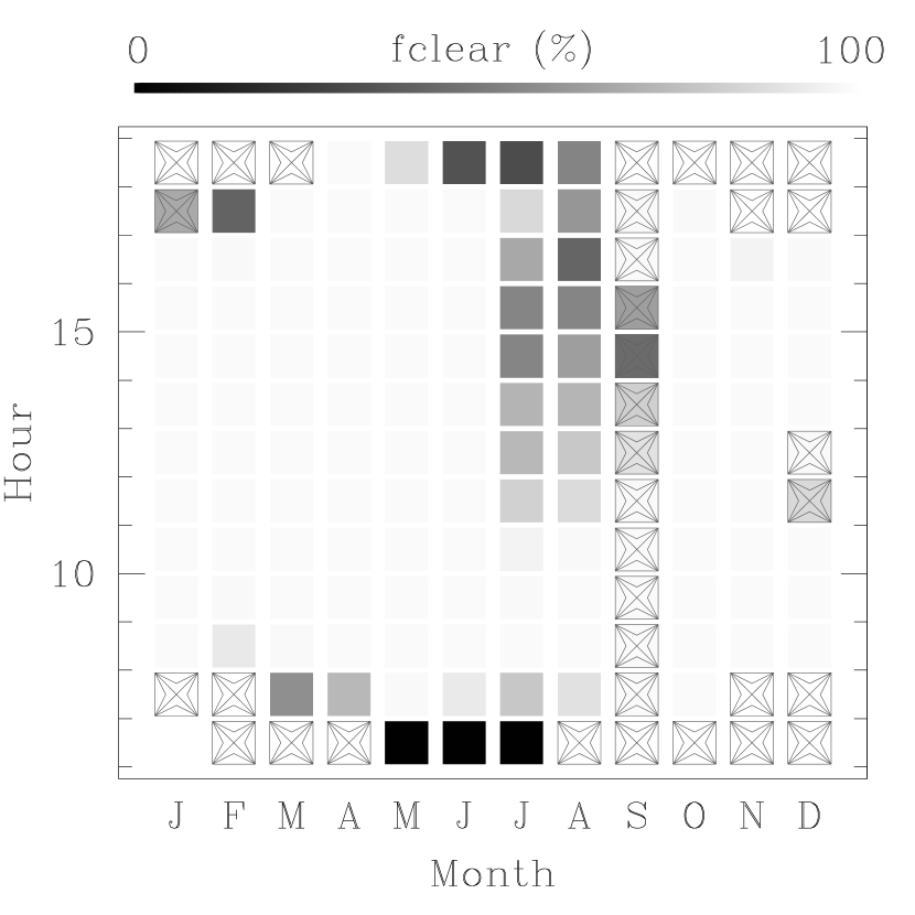
Figure 14: Grey level plot showing the median fraction of clear time for each month and hour of day. Squares are drawn when more than 10 hour of data are available; crosses indicate less than 10 hr of data.

Fig. 14 shows a grey level plot of the median percentage of clear time for a given combination of month and hour of day. Squares are drawn when more than 10 h of data are available; crosses indicate less than 10 h of data. Clear conditions are present in the colder and drier months, from October to June. Dark squares show cloudy weather, clearly dominant in the afternoons of the summer months, from July to September.

We repeated the analysis for airmass lower than 2. An equivalent histogram to that shown in Fig. 9, was created by computing the fraction of f(clear) for every hour, adding 5211 h. As expected, it also has an almost unimodal distribution: 82.5 per cent have f(clear) = 1 while 6.7 per cent of hours f(clear) = 0. The remaining fraction of data have intermediate values. The values of f(clear) obtained for the periodicities presented in this section are very similar but with less dispersion. In fact, in the analysis per hour the difference in median values are within 0.1 per cent. For the analysis per month the differences are also in that range except for July and August with differences between 0.3 to 13 per cent, with a maximum of 20 per cent for July 2006. The lower values obtained for the global distribution and for different periods can be explained by the presence of clouds formed at airmass $2<z<10$. The equivalent grey level plot of Fig. 14 for airmass less than 2 (not shown) does not include the contribution of clouds formed in the early morning and late afternoon hours, specially during the summer months.

7 Summary and conclusions

Using the solar radiation data recorded by the TMT site-testing group at SPM observatory, we applied a novel method developed by   Carrasco et al. (2009) to estimate the time when the sky is clear of clouds. From the global normalized observed distribution of $\psi$: the solar flux $F(t)$, divided by the nominal solar flux at the top of the atmosphere $F_{\sun}\cos\theta_{\sun}(t)$ we obtained that 82.4 per cent of the time the sky is clear of clouds for airmasses $z\leq 2$. This result is consistent within 6 per cent with the independent estimation of cloud cover using satellite data by  Erasmus & Van Staden (2002) who calculated a nighttime useful fraction of 81 per cent and estimated that the daily clear fraction is about 5 per cent less.

By analyzing the fits to the histograms of $\psi$ per month, we found that there is an annual seasonal effect: the centre of the clear peak has a maximum of 0.889 in February, reaches a minimum of 0.761 in July and increases to 0.885 towards the end of the year. As an example we presented the fits to the histograms for July and November obtained using the complete data set. The centre of the peak for July is 0.761 and for November is 0.841 but the amount of radiation corresponding to $\psi=0.761$ received at the site in July is 277 Wm^-2 more than that in November. This result is consistent with the seasonal variation in PWV measured at the site for several years obtained by Otárola et al. (2009) and Otárola et al. (2010). The difference can be explained by the presence of more aerosols in July that absorb the incident radiation in the atmosphere. Araiza & Cruz-González (2011) found that there are more aerosols during spring (maximum) and summer than in the rest of the year. These results suggest that when the sky is clear of clouds the value of $\psi_{0}$ is related to the atmosphere transparency.

For completeness we carried out a statistical analysis of the f(clear) for airmass lower than 10. First, we obtained a non symmetrical distribution of hourly clear time showing that 78.6 per cent of the time the sky is completely clear at this airmass interval. We calculated the first, second and third quartile of f(clear) for different periodicities. We presented the results for each month of the four-year observing period. An annual cycle is clearly noticeable: large fluctuations are observed mainly during the summer months. Big variations are also present for 2005 in January, February and December but this trend is not reproduced in 2006. The monthly distribution of f(clear) was obtained by combining the data of the same months for the whole period. The median of f(clear) is $\sim$ 0.99 between March and May, is relatively poor between June and September, with a minimum median value of about 0.72 in July, and fair during December and February. In addition, we calculated the quartiles of f(clear) as a function of hour of day using the complete data set: good conditions are more common in the mornings, f(clear) is highest before noon and decreases towards the afternoon. We also carried out the same analysis of hour of day for the seasons subset. It is apparent that the conditions are very stable for all the seasons except in the summer when there is more variability. To summarise our results we created a grey level plot, where f(clear) is represented by the grey intensity, indicating the median fraction of clear time for each month and hour of day: clear conditions exist in the colder and drier months, from October to June while cloudy weather is present in the afternoons of the summer months.

The fit to the histograms of $\psi$ developed by Carrasco et al. (2009) for Sierra Negra also reproduced the SPM data showing that this method might be generalized to other observatory sites. Furthermore, the consistency of our results with those obtained by other authors shows the great potential of our method as cloud cover is a crucial parameter for astronomical characterization of any site and can be estimated from in situ measurements.

References

- Araiza & Cruz-González (2011) Araiza M.R. & Cruz-González I., Rev. Mex. AA 2011, 47, 409
- Carrasco et al. (2009) Carrasco E., Carramiñana A, Avila R., Gutiérrez C., Avilés J.L., Reyes J. Meza J. & Yam. O., 2009, Mon. Not. R. Astron. Soc., 398, 407
- Cruz-González et al. (2003) Cruz-González I., Avila R. & Tapia M., eds, 2003, Rev. Mex. AA (SC), 19
- Cruz-González, et al. (2007) Cruz-González I., Echevarría J. & Hiriart D., eds, 2007, Rev. Mex. AA (SC), 31