Abstract

Many attempts to relate animal foraging patterns to landscape heterogeneity are focused on the analysis of foragers movements. Resource detection patterns in space and time are not commonly studied, yet they are tightly coupled to landscape properties and add relevant information on foraging behavior. By exploring simple foraging models in unpredictable environments we show that the distribution of intervals between detected prey (detection statistics) is mostly determined by the spatial structure of the prey field and essentially distinct from predator displacement statistics. Detections are expected to be Poissonian in uniform random environments for markedly different foraging movements (e.g. Lévy and ballistic). This prediction is supported by data on the time intervals between diving events on short-range foraging seabirds such as the thick-billed murre (Uria lomvia). However, Poissonian detection statistics is not observed in long-range seabirds such as the wandering albatross (Diomedea exulans) due to the fractal nature of the prey field, covering a wide range of spatial scales. For this scenario, models of fractal prey fields induce non-Poissonian patterns of detection in good agreement with two albatross data sets. We find that the specific shape of the distribution of time intervals between prey detection is mainly driven by meso and submeso-scale landscape structures and depends little on the forager strategy or behavioral responses.

Introduction

A number seabird species search and catch prey in ranges from hundreds to thousands of kilometers away from their nesting sites [1, 2, 3, 4, 5, 6, 7, 8]. The changing nature of marine environments makes seabird prey distributions highly dynamic and unpredictable over large spatial scales, ultimately impacting on seabirds capture efficiency [9, 10]. In this scenario, seabird populations are under constant survival pressure, a situation worsened by climate changes, that significantly perturb prey availability and the ecology of predator-prey systems [11, 12]. A well known example is the impact of El Niño-ENSO oscillations in the Pacific Ocean [13] on sardine population fluctuations off South Africa coast [8]. Studies of how seabirds detect and catch prey in the open ocean are also very important to assess the health of fish stocks [14, 15, 16, 17, 18], particularly for declining species that are commercially valuable [19, 20]. The availability of telemetry and satellite tracking technologies [21, 22, 23, 24, 25] accounts for recent progress in the understanding of habitat use and foraging behavior of long-range oceanic birds [26, 27]. Yet, this new empirical knowledge has been seldom followed up by theoretical studies providing general and more formal rationale for the observed foraging patterns. Motivated by this, and inspired by the long-range foraging patterns of albatrosses, here we explore how landscape-properties (i.e. large-scale prey spatial distributions) affect prey detection patterns in seabirds.

Foraging models (see, e.g. [28, 29, 30]) often examine the average distance (or time) travelled between successive prey detections, a key quantity that is inversely proportional to the foraging efficiency. Much less attention has been paid to the entire distribution of distances/times between detected prey (but see [30]), herein referred to as detection statistics. This latter quantity has been sometimes directly measured, in particular for wandering albatrosses (Diomedea exulans) [31, 10]. It is worth noting that detection patterns in unpredictable environments are -a priori- not closely related to displacement patterns. Displacements, i.e., a set of positions defining a trajectory, reflect internal states and complex behavioral responses to resource distributions [32, 33, 34, 35, 36, 37]. Detections, in turn, are localized events resulting from the explicit or physical interaction of the forager with the prey field and/or targeted landscape features.

For the past decade, a wide debate has focused on animal movement models with power-law move length distributions (Lévy walks) and on their possible interpretation as optimal search strategies of randomly distributed prey [38, 28, 39, 40, 41]. The movement patterns of many foragers, for instance, marine predators [37], plankton [42], spider monkeys [43] or jackals [44] display a wide range of spatial scales that cannot be accounted for by Poisson statistics. Wandering albatrosses were actually one of the first biological examples where evidence for Lévy displacements was reported [24, 28]. Flaws found later in the analysis questioned these findings and data of higher resolution were neither fitted by a Lévy law nor a Poisson law, but by a truncated modified power-law function [45]. This set of studies has attempted to draw conclusions on the search strategies of albatrosses not from direct position tracking, but based on flight duration data, which were assumed to be indicative of detection times between prey [24, 28, 45]. Here we provide further evidence showing that these data are actually related to detections, but also show that they do not carry information on movements and, therefore, on the nature of the search patterns leading to these detections.

We more generally examine the effects of the prey field spatial structure and of foraging rules on detection patterns. For prey uniformly distributed in space, detection patterns are trivially exponential if displacements are ballistic or self-avoiding but the outcome is less obvious for other types of movement. We find that Lévy movement models [28] also lead to exponential prey detection patterns in Poissonian environments, which illustrates the markedly different nature of detection and movement statistics. These predictions can explain the diving patterns of short-range foraging seabirds, such as the thick-billed murre [46], whose dives are exponentially distributed on time.

Prey in the ocean are not uniformly distributed at large scales, though [47, 48, 49, 50]. Detection patterns in complex media have been little studied and mostly in non-biological contexts [51]. We show that the non-Poissonian albatross data of [10] and [45] can be explained by models of a forager flying over a fractal prey landscape with parameter values consistent with observed resource distributions in the ocean. We use two models generating fractal landscapes of different nature and relate the fluctuations in the predator detection times (or distances) to the prey density heterogeneities. As in the uniform case, detection patterns in a given environment are found robust with respect to a variety of foraging rules, where the predator may or may not switch between different behaviors depending on prey detection.

Foraging seabirds: movement vs. detection statistics

In this study we re-analyze data from thick-billed murres and wandering albatrosses, two seabird species with markedly different behaviors. Thick-billed murres forage over small spatial scales in short foraging trips (representing less than 1h of flight in total) within a few kilometers of their colony [46]. They feed on benthic or pelagic fish in zones where prey occur in patch and are relatively predictable. These animals show a high degree of site fidelity. Murres perform above-water and underwater searching, although the latter has a much shorter mean duration [46]. In ref. [46], flight durations ($t$) of thick-billed murres between consecutive dives were measured with time-depth-temperature recorders.

On the other hand, telemetry data reveal that some albatrosses species, especially wandering albatrosses, perform exploratory trips of thousands of kilometers involving commuting and looping typical of central-place foraging [10, 52]. This large scale behavior is interspersed with hierarchically nested area-restricted search induced by the recognition of water masses such as the shelf edge, seamounts or frontal zones. Prey are likely to be scattered within these mesoscale physical structures that represent higher profitability areas that need to be prospected, involving successive landings and take-offs [52]. Heart-rate recorder signals in wandering albatrosses show that landings and take-offs represent a high energy expenditure for these large birds, who practically consume as much energy flying with a favorable tail or side wind as when sitting on the water or resting on the nest [53]. From an optimality standpoint landings should be considered informed behavioral responses, mostly associated to prey detection or exclusive seascape features, but not strictly related to successful prey captures. In [10, 54] it was observed that birds need about two landings on average before capturing prey (measured from stomach temperature sensors data). In particular, two capture modes have been identified in wandering albatrosses: “foraging in flight”, where the prey is captured within a few seconds after landing, and “sit-and-wait”, where the bird is sitting on the water for more than 10 min before prey is caught [31, 52]. The sit-and-wait strategy appears to be a secondary tactic used for prey clustered in small patches, for which foraging in flight would require high turning and landing rates, or for prey capture at night [52]. Albatrosses also land in water to rest, probably selecting the resting areas as well. Herein the term “prey detection” will denote the detection of prey, prey cues, or targeted seascape areas (for prospection, potential prey captures, resting, etc.) that may induce landing or diving responses.

One of the wandering albatross data discussed in the following (Bird Island data [45]) were obtained with wet-dry sensors measuring flight durations ($t$) between successive take-offs and landings. The data was acquired in 2004 with a reading each $\Delta t=$10s [45]. However this technology, which is similar to that of the murre data mentioned above, does not give information on trajectories and the animals were not equipped with a high resolution GPS device. The second wandering albatross data set re-analyzed here (Crozet Islands data [10]) consists in distances between captured prey measured using stomach temperature transmitters and position tracking systems.

Let us now consider, as an illustrative example, the search model of [28]. A forager with constant velocity $v$ chooses randomly oriented, rectilinear displacements of lengths ($l$) drawn from a probability distribution function (PDF) $P_{0}(l)$. Prey is immobile and randomly, uniformly distributed on a plane in number density $\rho$, and the forager can detect a prey only when it is at a shorter distance than a perception radius $r$. A step is stopped if a prey is detected on the way or completed otherwise.

Viswanathan et al. [28] considered power-law distributions, $P_{0}(l)=Cl^{-\mu}$ for $l>l_{0}$ and zero otherwise, where $1\leq\mu\leq 3$. To test this move length distribution for wandering albatrosses, [28] and [45] compared the PDF of the flight durations $t$ obtained from the wet-dry sensors to a power-law distribution. A similar comparison was performed with the flight duration data of the thick-billed murres [46]. In these studies, $t$ was thus assumed to be indicative of a chosen move length, $l$. But, as we have argued, $t$ represents the time elapsed between two detections, not a time spent traveling in straight line between two re-orientations. As $t$ and $l$ are different variables, they a priori obey different distributions. Therefore, comparing the model (or any other foraging model) with the three data sets described above requires to seek the PDF of the distance flown between two successive detected prey for that model, denoted as $L$ here (if the bird velocity is constant, then $L=vt$). Equivalently, $L$ is the sum of the step lengths travelled between prey. One may use the identity $PDF(L)=-dp(L)/dL$, where $p(L)$ is the probability that a path of length $L$ has not found a prey yet (or the fraction of flights of length $\geq L$).

Prey detections in Poissonian landscapes

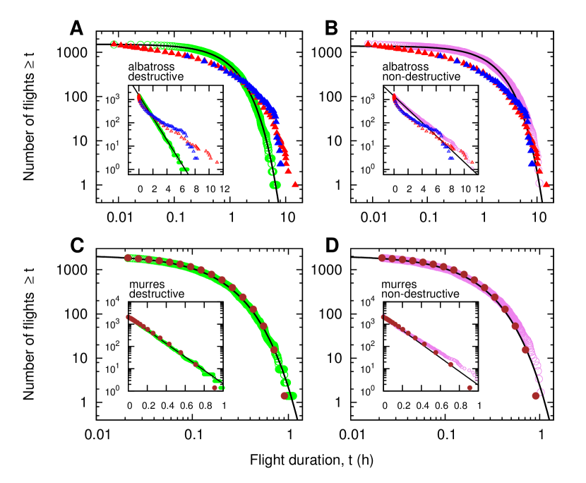
Figure 1: Detections in random uniform prey landscapes. (a) Albatross data and the model with destructive scenario. Green circles: accumulated distribution $p(L)$ of flight lengths between successive detected prey of the model forager [28] with perception radius $r$=0.001 following a Lévy process with $\mu$=1.5 (from 20 simulations of 75 captures each). The foraging ground is represented by a square of area unity and contained 5000 prey. Continuous line: exponential fit. Red triangles: $p(L)$ of the Bird Island albatross takeoff/landing data [45]. Blue triangles: $p(L)$ of the Crozet Islands albatross prey capture data [10], converted into flight durations assuming a constant flight velocity $v=16$m/s. Inset: same curves represented in semi-log to better emphasize the non exponential nature of the observed albatross data versus the exponential form of the model forager detections. (b) Albatross data and model with non-destructive scenario. Violet circles: accumulated distribution $p(L)$ for the model forager performing a Lévy process with $\mu$=2. Continuous line: exponential fit. Prey number: 3000; $r$=0.0003. In a) and b), the lengths in the model with foraging arena of area unity are converted in hours ($t$) by using $L=vt$ with the scaling factor $v$=0.12. Inset: same curves represented in semi-log to better emphasize the non exponential nature of the observed albatross data versus the exponential form of the model forager detections. (c) Murre data and model with destructive scenario. Green circles: accumulated distribution $p(L)$ of flight lengths between prey of the model forager with perception radius $r$=0.001 following a Lévy process with $\mu$=1.5 (from 20 simulations of 75 captures each). Continuous line: exponential fit. Brown dots are the murre flight durations from [46]. Inset: same data represented in semi-log in order to better emphasize the exponential nature of both the observed murres data and the model forager. (d) Murre data and model with non-destructive scenario. Violet circles: accumulated distribution $p(L)$ for a forager performing a Lévy process with $\mu$=2. Continuous line: exponential fit. Prey number: 3000; $r$=0.0003. Inset: same curves represented in semi-log. Similar close-to-exponential detections are obtained in all simulations with $1\leq\mu\leq 3$, in both destructive and non-destructive scenarii.

We illustrate below that the distance flown between to successive detection events, i.e. $L$, is exponentially distributed in random and uniform prey fields, even if the choice distribution $P_{0}(l)$ is not an exponential. In such landscapes, if detected prey disappear (destructive scenario), any foraging strategy producing paths that do not revisit the same location is optimal. Such non-oversampling paths can be ballistic (similar to a Lévy process with $\mu\approx 1$), spirals, self-avoiding walks, etc… Any non-oversampling path of length $L$ has a probability $p(L)=\exp(-L/\lambda)$ of not finding any prey, with $\lambda=1/(2r\rho)$ a characteristic distance, being $r$ a detection radius and $\rho$ the prey density. If the forager follows a random Lévy search, its trajectory involves some degree of oversampling. We have obtained $p(L)$ from numerical simulations for this model. In a destructive scenario, in which prey are depleted and not revisited, $p(L)$ closely follows an exponential, not only for $\mu\approx 1$ but also for walks with $1<\mu\leq 2$ (Figure 1a and c). In the non-destructive scenario, prey can be revisited. If one chooses $\mu=2$ or any smaller value, one also observes exponential detection statistics in a very good approximation (Figure 1b and d). The distribution $-dp(L)/dL$ has the form $\lambda_{d}^{-1}\exp(-L/\lambda_{d})$, a shape which is not related to that of $P_{0}(l)$. These results illustrate that exponential tails for prey detection statistics are an essential outcome of foraging models, including those generated from Lévy processes, when the landscape is Poissonian. However, the precise value of the characteristic length travelled between prey, $\lambda_{d}$ (which is related to the foraging efficiency), generally depends on the scenario and movement rules ($P_{0}(l)$, here). As we assume that movement is truncated by detections, $\lambda_{d}$ is finite.

The simple exponential form of $p(L)$ obtained for uniform prey fields describes well the murre data. The maximum likelihood estimate (MLE) of $\lambda_{d}$ is $9.5$min and a log-likelihood ratio test of goodness-of-fit (G-test) was performed from $10^{4}$ independent Monte Carlo samplings, giving $P=0.82$ ($n=2083$, $df=15$). In contrast, the exponential does not describe none of the wandering albatross curves, see Figure 1 (G-test, Bird Island: $P<$ 0.0001, $n$= 1507, $df=47$; Crozet Islands: $P<0.0001$, $n=276$, $df=47$). In this figure, distances in the Crozet I. data were converted into flight durations assuming a constant flight velocity $v=16$m/s [55, 52]. The resulting curve lies very close to the Bird Island data.

Prey detection in large scale fractal landscapes

In the case of Bird Island wandering albatrosses, Edwards et al. accurately fitted the flight duration distribution by a shifted gamma function, which is asymptotically an exponential multiplied by an inverse power-law [45]. Similarly, Weimerskirch et al. found that the distribution of distances between captured prey by Crozet Islands wandering albatrosses did not follow a simple exponential, but approximately an inverse power-law [10] (see also [56]).

Such intermittent landing by albatrosses, often related to prey capture behaviour, can be explained by fractal prey landscapes. As a matter of fact, wandering albatrosses forage over much larger spatial scales than murres and mainly feed on squid and pelagic fish [10]. This prey display several levels of spatial aggregation and schooling [47, 48] and have strong spatial overlap with plankton [49]. The large scale horizontal spatial distributions of plankton [50, 37], passive drifters [57], cephalopods [47] and pelagic fish [58, 59, 48, 60] are known to be self-similar (with fractal dimension $D_{F}\approx 1.2-1.6<2$) over a wide range of scales, typically from a lower characteristic scale $R_{0}$, of tens of meters, to an upper scale $R_{m}$, of 100$-$300 km [50, 58, 60]. At scales larger than $R_{m}$ the prey field is seen as heterogeneous but space filling, that is, with $D_{F}\approx 2$. The mechanisms generating fractal horizontal distribution of marine species near the ocean surface are not well-known. Oceanic turbulence [60, 50] and predator-prey interactions [61] are two factors often invoked.

Based on these field observations, we consider below more realistic prey distribution models that generate fractals of different types.

(a) Truncated Lévy Dust model (LD)

It is commonly accepted that the assumption of randomly distributed prey in spatial ecological models is not entirely appropriate since there is a growing body of evidence showing that prey are more likely distributed in a patchy and aggregated fashion. This seems to be especially true for distributions of prey in marine environments as discussed above [58, 59, 48, 60]. Lévy dusts in finite domains are a convenient method to generate stochastic fractal point patterns and they have been applied to model oceanic prey fields [50, 37]. They have been less often used to model the movement of foragers profiting on these, though (but see [62]). Our first fractal foraging model therefore employs truncated Lévy dusts (LD) to generate fractal prey locations.

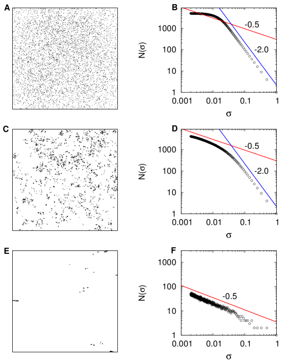
Figure 2: Three different theoretical patterns of spatial prey distribution in a unit box and their corresponding box-counting fractal dimension. $\sigma$ represent the size of the boxes and $N(\sigma)$ is the number of boxes of size $\sigma$ in the box-counting algorithm. In the three cases, 5000 prey are distributed accordingly to a Lévy dust with fractal dimension $D_{F}=0.5$ ($\beta=1.5$). (a) If the minimal distance between prey is large the Lévy process producing the fractal pattern bounces many times on the walls and the overall process tends to be space-filling. In this particular case, the minimal distance between prey was $1/7$ and the process bounced around 2500 times which is equivalent to the superposition of 2500 separated fractals in the same domain. (b) As expected in this case, the fractal dimension measured by box-counting does not show a scaling region with exponent $D_{F}=0.5$ (red line) but approximates more the typical graph of a 2D random process with $D_{F}=2.0$ (blue line). (c) Pattern that corresponds to a prey distribution with a minimal distance of $1/700$ between prey, leading to less than 150 bounces ( 3% of the total prey number). (d) In this case a scaling region with $D_{F}=0.5$ is visible, followed by a two-dimensional behavior at larger length scales. (e) A very clumped and aggregated fractal pattern of prey is obtained when the minimal distance between prey is set to $7\times 10^{-6}$. (f) In this case the fractal is nearly perfect with $D_{F}=0.5$.

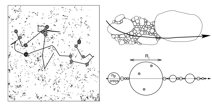
Figure 3: Left panel. Foraging arena composed of $N$=5000 prey generated with a LD of exponent $\beta$=1.5 (fractal dimension $D_{F}$=0.5). Solid line: trajectory of a ballistic forager ($\mu\simeq 1$) with detection radius $r$=0.001. The larger grey dots indicate detection events (destructive scenario). Right panels: Fractal Local Density (FLD) model. Upper figure: The medium is composed of patches of heterogeneous sizes $R$, drawn from a PDF $\psi(R)\propto R^{-\nu}exp(-R/R_{m})$. Within a patch, $n_{p}(R)\propto R^{\epsilon}$ prey are randomly and uniformly distributed. Lower figure: linear representation of the forager/medium system, which is solved here.

LD are standard Lévy flights coming from the power-law distribution $f(x)\sim x^{-\beta}$ with $1<\beta\leq 3$ [63] and where only the turning points joining successive displacements $x$ are considered as prey locations. This method generates point patterns with fractal dimension $D_{F}=\beta-1<2$ (Figure 2). The power-law distribution when finite (contained in a square domain-box of unit length) is truncated in the range $[\delta,1]$ where $\delta$ is interpreted as the minimum distance separating neighboring prey. On the other hand, the maximum distance separating consecutively located prey is the domain-box size, set to 1 for convenience. Between both limits (which define the self-similarity range of the fractal) the corresponding truncated probability distribution function is normalized to 1. The Lévy dust generator starts at the center of a square domain of unitary area and accommodates $N$ successive prey (see Figure 2). When a new prey position is to be located outside of the domain, it is discarded and a new step is attempted (we call this a “border-bounce”). The fractal nature of the pattern may disappear if the number of bounces is too high. In order to prevent this, a tuning of $\delta$ is applied to guarantee that the number of bounces is low, given a total number of prey. If the distance $\delta$ is large enough (but always $\ll 1$) and if the total number of prey is also large, the pattern approximates a Poisson distribution because of too much bouncing. If the value of $\delta$ is too small, the prey field is limited to a very small region of the domain. An intermediate situation would produce a locally sparse fractal covering the whole domain. In our simulations, we took values of $\delta$ such that a bounce occurs in no more than 1.5% of the total number of prey. It is also necessary to keep in mind that the value of $\delta$ depends on the value of the scaling exponent $\beta$ of the walker. The lower the exponent $\beta$ is, the lower the value of $\delta$ has to be in order to generate an undistorted fractal with few bounces (see Figure 2). We will discuss in the following section the detection dynamics of a forager moving on a fractal prey field generated by this process (see Figure 3, left).

(b) Fractal Local Density (FLD) model

We next propose an alternate and original model that builds stochastic fractals where, in contrast with Lévy dusts or Sierpinski-like hierarchical structures [58, 51], the local prey density $\rho$ is well-defined.

Acoustic devices allow to measure the density of marine organisms, either locally (e.g.,[37]) or over hundreds of kilometers squared instantaneously [60]. Krill density has been observed to fluctuate widely from one location to another and to follow a power-law frequency distribution, of the form $PDF(\rho)\sim\rho^{-\alpha_{\rho}}$, with $\alpha_{\rho}\approx 1.7$ [37]. These large density variations also have a spatial structure that involves many length scales across the landscape [60]. Therefore, to characterize the prey field as a patchwork of regions with different densities, one must specify the sizes of these regions. These length scales ($R$ below) represent an other important ingredient of the model, as the local density alone is not a space variable. For albatrosses, fairly localized high productivity marine areas occur interspersed with vast oceanic areas of low productivity [10, 54]. We construct a model that captures these properties. In the model, high density regions are numerous but small, and represent overall a small fraction of the total area, corresponding to the tail of the density PDF. On the contrary, a significant area fraction is occupied by a few large regions of very low local density. The density is a continuous variable bounded by a minimal and a maximal value.

The definition of a patch tends to be rather inclusive. We define here a patch as a region of space of uniform prey density, with no limitation on its size and density [64, 65]. Consider a random assembly of non-overlapping, roughly circular patches of varying diameters $R$ that are drawn from a frequency distribution $\psi(R)$ (Figure 3, right). Inside a patch of size $R$, an average number of $n_{p}(R)$ prey are distributed randomly and uniformly. Therefore, the density in a patch is proportional to $n_{p}(R)/R^{2}$. To obtain a medium with fractal properties up to a scale $R_{m}$, one first distributes $R$ according to a truncated power-law distribution:

$$\psi(R)=cR^{-\nu}\exp(-R/R_{m}),\quad{\rm with}\ R\geq R_{0}$$ (1)

where $\nu$ is an exponent related to the fractal dimension, $R_{m}$ the large cut-off length of the fractal mentioned earlier, and $c$ the normalization constant. In addition, $R$ is always larger than some length $R_{0}$, which is the minimum size of a patch $(R_{0}\ll R_{m})$ and can be taken as the resolution size. We next assume an algebraic relationship between the size of a patch and the number of prey it contains:

$$n_{p}(R)=kR^{\epsilon},$$ (2)

with $k$ a constant and $\epsilon$ an exponent $\leq 2$. The case $\epsilon=2$ corresponds to a uniform Poissonian medium, where all regions have the same density. As further shown, the albatross data is best fitted by landscapes with negative values of $\epsilon$: large patches have fewer prey. On length scales $R_{0}<R\ll R_{m}$, the patch distribution (1) is scale-free, whereas practically no patch has a size much larger than $R_{m}$. The box-counting method shows that for some parameters $\nu$ and $\epsilon$, the prey distribution of this model forms a fractal set with dimension $D_{F}<2$ on scales smaller than $R_{m}$ (see Supplementary Information). Restricting ourselves to the case $\epsilon<0$ of interest here, one finds that the fractal dimension is given by:

$$D_{F}=\nu-\epsilon-1<2,\quad{\rm for}\ \nu<3+\epsilon,$$ (3)

whereas $D_{F}=2$ for $\nu>3+\epsilon$. When $D_{F}<2$, the PDF of the local prey density is an inverse power-law (over a wide range of densities provided that $R_{m}/R_{0}$ is sufficiently large), with exponent given by:

$$\alpha_{\rho}=\frac{5-\epsilon-\nu}{2-\epsilon}>0.$$ (4)

In this medium, we consider the case of a ballistic predator with constant velocity $v$. Ballistic motion is the simplest movement behavior and can accurately represent albatross relocations at certain scales [31, 54]. If we assume that there are no correlations between the sizes of neighboring patches, the problem can be simplified to that of a forager flying through a one-dimensional succession of patches (Figure 3, right). The process is easy to simulate numerically: during an elementary time step $\Delta t$(=10s, as in [45]), the forager located in a patch of size $R_{i}$ travels a distance $R_{0}=v\Delta t$ and has therefore a Poissonian probability $\exp[-\tilde{r}(R_{i}/R_{0})^{\epsilon-2}]$ of not finding any prey, with $\tilde{r}=2rv\Delta tkR_{0}^{\epsilon-2}$ the dimensionless detection radius and $R_{i}/R_{0}$ the dimensionless patch size. The process is iterated until the end of a patch is reached, when a new $R_{i}$ (and therefore a new prey density) is drawn from Equation 1.

After a prey is detected, the forager can either (i) follow its way (“non-responsive search”) or (ii) stay within the same patch for $R_{i}/R_{0}$ other elementary time steps (“responsive search”). The latter rule mimics area restricted search [33, 30], a behavior that has been observed in wandering albatrosses [31, 54]. With rule (ii), the forager tends to exploit more intensively higher density regions, where detections are more probable.

Results

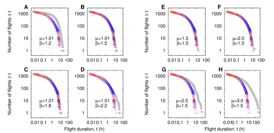
Figure 4: Detections in LD media. (a)-(d): Accumulated histograms of prey detection times (grey circles) for a ballistic model predator ($\mu$=1.01) with $r$=0.0003 foraging in LD environments ($N$=5000) of varying fractal dimension at lower scales. Foraging is destructive in all cases. Bird Island data: red triangles, Crozet Islands: blue triangles. Recall that $D_{F}=\beta-1$. (a) $\beta$=1.2 ($\delta=5\times 10^{-7}$, $v$=0.55), p-value of K-S test on Bird Island: $p_{B}$=0.0045, Crozet Islands: $p_{C}$=4.9e-08; (b) $\beta$=1.5 ($\delta=2\times 10^{-4}$, $v$=0.50), $p_{B}$= 0.997, $p_{C}$=0.248; (c) $\beta$=1.8 ($\delta=1.67\times 10^{-3}$, $v$=0.25), $p_{B}$= 0.997, $p_{C}$= 0.367 and (d) $\beta$=2.2 ($\delta=3.84\times 10^{-3}$, $v$=0.20), $p_{B}$= 0.033, $p_{C}$= 0.033. (e)-(h): Same quantities for LD media with fixed $\beta$=1.5 ($N$=5000, $\delta=2\times 10^{-4}$) and a model forager following processes with different step length distributions: (e) $\mu$=1.5 ($v$=0.5), $p_{B}$= 1, $p_{C}$= 0.248; (f) $\mu$=2.0 ($v$=0.67), $p_{B}$= 0.999, $p_{C}$= 0.0995; (g) $\mu$=2.5 ($v$=0.67), $p_{B}$= 0.000955, $p_{C}$=4.03e-09 and (h) $\mu$=3.0 ($v$=0.67), $p_{B}$= 6.38e-05, $p_{C}$= 1.72e-13.

A ballistic walker foraging through a LD with $0.5\leq D_{F}\leq 0.9$ (corresponding to $1.5\leq\beta\leq 1.9$) produces a flight duration distribution that fits very well the Bird Island [45] and Crozet Islands [10] albatross data over the entire range (Figure 4a-d). Somewhat surprisingly, no fine tuning of the fractal dimension is needed, as a range of small values of $D_{F}$ describes the data equally well. In contrast, Lévy dust landscapes with $D_{F}<0.5$ or $D_{F}>0.9$ do not produce a good agreement with empirical data. In a given landscape, detection patterns are also robust to changes in the assumptions regarding predator movements. If predators, instead of being ballistic ($\mu\approx 1$), choose step lengths with $1\leq\mu\leq 2$, for instance $1.5$ and $2$, $p(L)$ in Figure 4e-h still fits the data very well (LD with $D_{F}=0.5$). Poor agreement is obtained for $\mu=2.5$ and larger, therefore, albatross data cannot be explained by a Gaussian random walker detecting prey in a fractal media. While a LD fractal prey field gives detection statistics that are qualitatively in excellent agreement with the observed albatross data, estimations of $D_{F}$ for oceanic prey fields are indeed in the range $1.2<D_{F}<1.6$ [57, 50, 59]. This quantitative difference prompts us to analyze the FLD model where good agreement can be obtained with $D_{F}$ in this range of values.

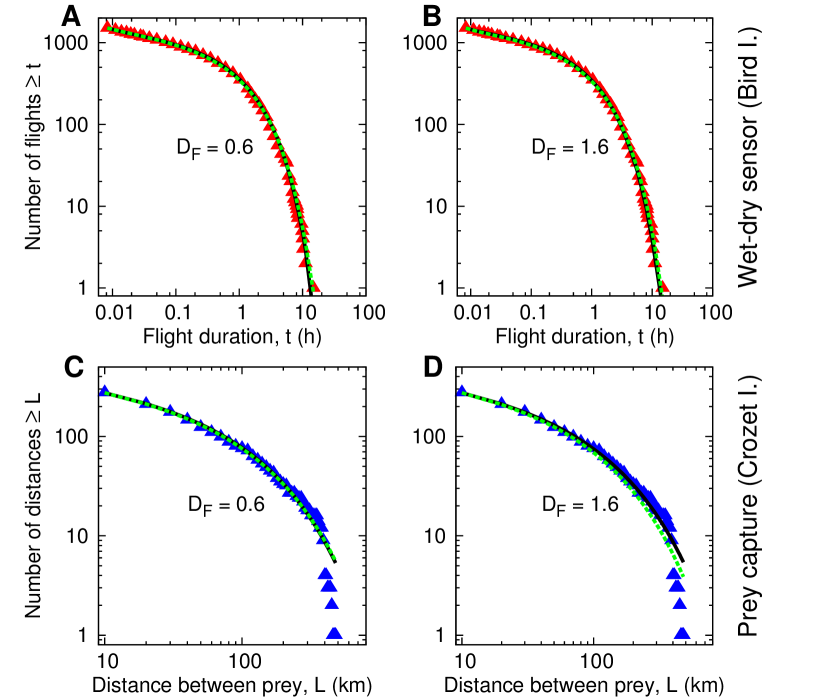
Figure 5: Cumulative distribution of prey detection times/distances obtained by fitting the FLD model to the albatross data (triangles), for two fixed fractal dimensions of the medium ($D_{F}$=0.6 and 1.6). Solid black line: responsive search; green dotted line: non-responsive search. Each curve is plotted with the MLE of the parameters, see Table 1. (a)-(b): Bird Island. (c)-(d): Crozet Islands. The best estimates of the patch size distribution parameters vary little in the different cases: $\nu$=1.20 $\pm$ 0.05 and $R_{m}$ in the range of 160-240 km, independently of $D_{F}$, for the whole range considered. A more efficient strategy yields a lower dimensionless detection radius $\tilde{r}$.

The FLD model gives similar results (Figure 5). First, a range of values of the fractal dimension can fit the data. Secondly, the different foraging behaviors considered can fit the data, too. Table 1 displays, for various values of $D_{F}$ and forager behaviors, the maximum likelihood estimates (MLE) of the exponent $\nu$ of the patch size distribution, of the cut-off length $R_{m}$, and of the dimensionless detection radius $\tilde{r}$. The responsive search scenario describes the data as well as the simple ballistic one. The main difference between the two cases is the value of $\tilde{r}$. The responsive case is much more efficient since the same prey detection patterns are obtained by a forager with detection radius $(\tilde{r})$ 2$-$20 times smaller compared with a non-responsive forager in the same medium.

Importantly, within each data set the MLE of the patch size distribution parameters ($\nu$ and $R_{m}$) are nearly independent of $D_{F}$ and the foraging scenario. The parameter values found are also strikingly similar across the two albatross data sets. Using an estimate of albatrosses’ speed, 16 m/s [55, 52], the Bird Island flight durations were converted into km. The values of $R_{m}$ in Table 1 are of the same order of magnitude as the self-similarity range found in marine landscapes [50, 58, 59, 60]. Even by assuming that the Bird Island data are accurate for flights longer than $3\Delta t$=30s [45] or 480m, these values indicate that the albatross prey field is fractal over nearly three logarithmic decades.

In summary, our fractal landscape model produces non-exponential detection patterns and can explain wandering albatross data with realistic parameters. A non-trivial result is that the shape of the flight durations PDF is primarily determined by the patch size distribution $\psi(R)$, rather than by the fractal dimension $D_{F}$. Similarly to the robustness observed in the LD model, the shape of $p(L)$ in the FLD model is not altered by modifications in the forager movement strategy.

Discussion

The foregoing results show the importance of considering predator displacements and prey detection events in unpredictable environments as two different aspects of the same foraging process. We emphasize that detection patterns alone are in general unlikely to inform on movement patterns and search strategies. Detection statistics of long-ranging foraging animals in the ocean can be regarded as depending on the size of the regions with uniform density, i.e. a higher level of landscape organization, and not on all the details of the prey field. This result resonates with the current view that marine animals can track meso and submeso-scale seascape features [66]. Our study suggests that detection statistics in both uniform and scale invariant landscapes depend little on the hypothesized predator movement rules, therefore forager search strategies cannot be inferred from detection patterns only.

Wandering albatrosses adjust their movement to cope with overdispersed preys and environmental features at different scales [10, 54]. The two data sets analyzed here can be consistently explained by different foraging models assuming that landings and prey capture are related to prey detection and that prey is fractally distributed from about 200-400m up to scales of 150$-$250 km. These scales are in agreement with observations of the distributions of pelagic fish, plankton and squid in the ocean [50, 58, 60]. We infer that albatross prey distribution can be pictured as a random, self-similar assembly of regions with varying sizes and densities (FLD model). The empirical PDF of flight lengths is well reproduced if the size of the aforementioned regions follows a power-law distribution with exponent close to unity ($\nu\approx 1.2$, see Table 1). The truncation of very long flights ($>$200 km) is unavoidable as the prey field tends to be space filling beyond these scales. Our results on landing/take-off activity are consistent with direct prey capture data of wandering albatrosses, suggesting that both are closely related, although not strictly equivalent.

The probability distribution function of the local density of krill, the prey of several top marine predators, is described by an inverse power-law, $\rho^{-\alpha_{\rho}}$, with $\alpha_{\rho}\approx 1.7$ over four decades [37]. It is likely that many other types of organisms, in particular large fish, follow a similar pattern [60]. In the FLD model, along with $\nu$, $\alpha_{\rho}$ is an important exponent characterizing the prey field. In the two examples of Figure 5-Table 1, where $D_{F}$ is fixed to 0.6 and 1.6, respectively, we obtain $\alpha_{\rho}$=1.75 and 1.53 from relation (4). These values are comparable to the empirical exponent 1.7. These results also imply considerable relative variations in albatross prey density, at least of the order of $(R_{m}/R_{0})^{2}\approx 10^{6}$.

Large fluctuations in prey density have been identified as a possible cause of non-exponentially distributed detections [67]. The FLD model shows that it is indeed the case, if the local density fluctuations are structured in widely different characteristic sizes across many scales. As an example, in the ocean, high productivity areas are separated by larger areas of lower productivity [10, 54]. A simple analytical calculation can show that a forager crossing an heterogeneous medium composed of patches of equal and small sizes, although with power-law distributed prey densities, has an exponential $p(L)$ [68]. Hence, not only prey density distributions but the spatial arrangement of prey density fluctuations seem to be a crucial element to obtain non-exponentially distributed detections. In a different context, the study of a model of ballistic particles propagating through Sierpinski-like fractals showed that detection patterns were not exponentials [51]. Our modeled landscapes differ from these Sierpinski gaskets, though, as the fractals considered here are not characterized by a single length scale between nearest prey, an important assumption made in [51]. As noted earlier, no general relation has to be expected between the fractal dimension and detection statistics, which also depend on the kind of fractal structure considered.

Our results also show that random but uniform prey fields should lead to exponential detection patterns. We have identified exponential distributions of flight durations between dives in the thick-billed murre, an Arctic seabird that, unlike the much bigger wandering albatross, forages at small spatiotemporal scales by restricting its search over reduced areas where prey predictability is higher [46]. These observations can be interpreted within our modeling framework: a forager with a high degree of site fidelity performing a search restricted to areas where prey encounter is high should not experience large variations in prey density. Therefore, the detection patterns should come closer to an exponential form than for a species searching over vast oceanic surfaces.

We conclude that detection statistics, along other behavioral traits of seabirds [15], can give valuable information on the prey field spatial distributions. Namely, in our examples the frequency distribution of detection times or distances follow a scaling law, $\lambda_{d}^{-1}f(L/\lambda_{d})$, where $\lambda_{d}$ is a typical length between prey detections and depends both on predator movements and the prey field, whereas $f(x)$ depends on the prey field only. The function $f(x)$ is typically an exponential for uniform prey fields and may involve power-law terms for fractal media. These findings could be useful for disentangling the renewed debate on how organism-environment interactions build up statistical patterns of movement [29, 36, 40, 39] not only in seabirds but in other animals as well.

Tables

Table 1: Maximum likelihood estimates of the Fractal Local Density model parameters ($\nu$, $R_{m}$ and $\tilde{r}$) in several scenarii, for each albatross data set. (Note: in the Bird I. case, $R_{m}$ was obtained by converting flight durations into distances assuming $v=16$m/s [55, 52].)

		$\nu\quad$	$R_{m}$(km)	$\tilde{r}$	$\epsilon$	($P$, $G$)
Bird Island [45]	(wet-dry sensor data)
$D_{F}$=0.6	responsive search	1.2	160	1.8	-0.4	(0.69, 43.0)
$"$	non-responsive search	1.15	180	9.8	-0.45	(0.56, 46.0)
$D_{F}$=1.6	responsive search	1.2	160	5.4	-1.40	(0.51, 47.3)
$"$	non-responsive search	1.15	180	180	-1.45	(0.58, 45.6)
Crozet Islands [10]	(prey capture data)
$D_{F}$=0.6	responsive search	1.2	220	5.4	-0.4	(0.08, 62.3)
$"$	non-responsive search	1.2	240	13.6	-0.4	(0.09, 61.8)
$D_{F}$=1.6	responsive search	1.25	240	6.0	-1.35	(0.07, 62.0)
$"$	non-responsive search	1.2	210	160	-1.40	(0.04, 65.0)

Figure Legends

References

- 1. Prince PA, Francis MD (1984) Activity budgets of foraging gray-headed albatrosses. Condor 86: 297–300.
- 2. Cairns DK, Bredin KA, Montevecchi WA (1987) Activity budgets and foraging ranges of breeding Common Murres. The Auk 104: 218–224.
- 3. Irons DB (1998) Foraging area fidelity of individual seabirds in relation to tidal cycles and flock feeding. Ecology 79: 647–655.
- 4. Grémillet D, Dell’Omo G, Ryan PG, Peters G, Ropert-Coudert Y, et al. (2004) Offshore diplomacy, or how seabirds mitigate intra-specific competition: a case study based on GPS tracking of Cape gannets from neighbouring colonies. Marine Ecology Progress Series 268: 265–279.
- 5. Berrow SD, Wood AG, Prince PA (2000) Foraging location and range of white-chinned petrels Procellaria aequinoctialis breeding in the South Atlantic. Journal of Avian Biology 31: 303–311.
- 6. González-Solís J, Croxall JP, Wood AG (2000) Foraging partitioning between giant petrels Macronectes spp. and its relationship with breeding population changes at Bird Island, South Georgia. Marine Ecology Progress Series 204: 279–288.
- 7. Wood AG, Naef-Daenzer B, Prince PA, Croxall JP (2000) Quantifying habitat use in satellite-tracked pelagic seabirds: application of kernel estimation to albatross locations. Journal of Avian Biology 31: 278–286.
- 8. Crawford RJM, Sabarros PS, Fairweather T, Underhill LG, Wolfaardt AC (2008) Implications for seabirds off South Africa of a long-term change in the distribution of sardine. African Journal of Marine Science 30: 177–184.
- 9. Weimerskirch H, Le Corre M, Jaquemet S, Marsac F (2005) Foraging strategy of a tropical seabird, the red-footed booby, in a dynamic marine environment. Marine Ecology Progress Series 288: 251–261.
- 10. Weimerskirch H, Gault A, Cherel Y (2005) Prey distribution and patchiness: factors in foraging success and efficiency of wandering albatrosses. Ecology 86: 2611–2622.
- 11. Sydeman WJ, Hester MM, Thayer JA, Gress F, Martin P, et al. (2001) Climate change, reproductive performance and diet composition of marine birds in the southern California Current system, 1969-1997. Progress in Oceanography 49: 309–329.
- 12. Weimerskirch H, Louzao M, de Grissac S, Delord K (2012) Changes in wind pattern alter albatross distribution and life-history traits. Science 335: 211–214.
- 13. Mysak LA (1986) El Niño, interannual variability and fisheries in the northeast Pacific Ocean. Canadian Journal of Fisheries and Aquatic Sciences 43: 464–497.
- 14. Cairns DK (1992) Bridging the gap between ornithology and fisheries science: use of seabird data in stock assessment models. Condor 94: 811–824.
- 15. Monaghan P (1996) Relevance of the behaviour of seabirds to the conservation of marine environments. Oikos : 227–237.
- 16. Frederiksen M, Mavor RA, Wanless S (2007) Seabirds as environmental indicators: the advantages of combining data sets. Marine Ecology-Progress Series 352: 205–211.
- 17. Piatt JF, Sydeman WJ, Wiese F (2007) Introduction: a modern role for seabirds as indicators. Marine Ecology Progress Series 352: 199.
- 18. Einoder LD (2009) A review of the use of seabirds as indicators in fisheries and ecosystem management. Fisheries Research 95: 6–13.
- 19. Pauly D, Alder J, Bennett E, Christensen V, Tyedmers P, et al. (2003) The future for fisheries. Science 302: 1359.
- 20. Myers RA, Worm B (2003) Rapid worldwide depletion of predatory fish communities. Nature 423: 280–283.
- 21. Jouventin P, Weimerskirch H (1990) Satellite tracking of wandering albatrosses. Nature 343: 746-748.
- 22. Prince PA, Wood AG, Barton T, Croxall JP (1992) Satellite tracking of wandering albatrosses (Diomedea exulans) in the South Atlantic. Antarctic Science 4: 31–36.
- 23. Weimerskirch H, Salamolard M, Sarrazin F, Jouventin P (1993) Foraging strategy of wandering albatrosses through the breeding season: a study using satellite telemetry. The Auk 110: 325–342.
- 24. Viswanathan GM, Afanasyev V, Buldyrev SV, Murphy EJ, Prince PA, et al. (1996) Lévy flight search patterns of wandering albatrosses. Nature 381: 413–415.
- 25. Phillips RA, Silk JRD, Croxall JP, Afanasyev V, Briggs DR (2004) Accuracy of geolocation estimates for flying seabirds. Marine Ecology Progress Series 266: 265–272.
- 26. Weimerskirch H, Wilson RP (2000) Oceanic respite for wandering albatrosses. Nature 406: 955–956.
- 27. Louzao M, Navarro J, Forero MG, Igual JM, Genovart M, et al. (2011) Exploiting the closest production area: geographi-cal segregation of foraging grounds in a critically endangered seabird. Marine Ecology Progress Series 429: 291–301.
- 28. Viswanathan GM, Buldyrev SV, Havlin S, Da Luz MGE, Raposo EP, et al. (1999) Optimizing the success of random searches. Nature 401: 911–914.
- 29. Benhamou S (2007) How many animals really do the Lévy walk? Ecology 88: 1962–1969.
- 30. Plank MJ, James A (2008) Optimal foraging: Lévy pattern or process? Journal of The Royal Society Interface 5: 1077.
- 31. Weimerskirch H, Wilson RP, Lys P (1997) Activity pattern of foraging in the wandering albatross: a marine predator with two modes of prey searching. MEPS 151: 245–254.
- 32. Hassell MP, May RM (1974) Aggregation of predators and insect parasites and its effect on stability. The Journal of Animal Ecology 43: 567–594.
- 33. Benhamou S, Bovet P (1989) How animals use their environment: a new look at kinesis. Animal Behaviour 38: 375–383.
- 34. With KA, Cadaret SJ, Davis C (1999) Movement responses to patch structure in experimental fractal landscapes. Ecology 80: 1340–1353.
- 35. Fritz H, Said S, Weimerskirch H (2003) Scale–dependent hierarchical adjustments of movement patterns in a long–range foraging seabird. Proceedings of the Royal Society of London Series B: Biological Sciences 270: 1143.
- 36. Nathan R, Getz WM, Revilla E, Holyoak M, Kadmon R, et al. (2008) A movement ecology paradigm for unifying organismal movement research. Proceedings of the National Academy of Sciences 105: 19052.
- 37. Sims D, Southall E, Humphries N, Hays G, Bradshaw CJA, et al. (2008) Scaling laws of marine predator search behaviour. Nature 451: 1098–1102.
- 38. Shlesinger MF, Klafter J (2000) Lévy walks versus lévy flights. In: Stanley H, Ostrowsky N, editors, On Growth and Form: Fractal and Non-Fractal Patters in Physics. Dordrecht: Martinus Nijhoff Publishers, pp. 279–283.
- 39. Bartumeus F (2009) Behavioral intermittence, Lévy patterns, and randomness in animal movement. Oikos 118: 488–494.
- 40. Reynolds AM, Rhodes CJ (2009) The Lévy flight paradigm: random search patterns and mechanisms. Ecology 90: 877–887.
- 41. de Jager M, Weissing F, Herman P, Nolet B, van de Koppel J (2011) Lévy walks evolve through interaction between movement and environmental complexity. Science 332: 1551.
- 42. Bartumeus F, Peters F, Pueyo S, Marrasé C, Catalan J (2003) Helical Lévy walks: adjusting searching statistics to resource availability in microzooplankton. Proceedings of the National Academy of Sciences of the United States of America 100: 12771.
- 43. Ramos-Fernandez G, Mateos JL, Miramontes O, Cocho G, Larralde H, et al. (2004) Lévy walk patterns in the foraging movements of spider monkeys (Ateles geoffroyi). Behavioral Ecology and Sociobiology 55: 223–230.
- 44. Atkinson RPD, Rhodes CJ, Macdonald DW, Anderson RM (2002) Scale-free dynamics in the movement patterns of jackals. Oikos 98: 134–140.
- 45. Edwards AM, Phillips RA, Watkins NW, Freeman MP, Murphy EJ, et al. (2007) Revisiting Lévy flight search patterns of wandering albatrosses, bumblebees and deer. Nature 449: 1044–1048.
- 46. Hamish Elliott K, Bull RD, Gaston AJ, Davoren GK (2009) Underwater and above-water search patterns of an arctic seabird: reduced searching at small spatiotemporal scales. Behavioral Ecology and Sociobiology 63: 1773–1785.
- 47. Rodhouse PG, Prince PA, Trathan PN, Hatfield EMC, Watkins JL, et al. (1996) Cephalopods and mesoscale oceanography at the Antarctic Polar Front: satellite tracked predators locate pelagic trophic interactions. Marine ecology progress series Oldendorf 136: 37–50.
- 48. Fréon P, Cury P, Shannon L, Roy C (2005) Sustainable exploitation of small pelagic fish stocks challenged by environmental and ecosystem changes: a review. Bulletin of Marine Science 76: 385–462.
- 49. Garrison LP, Michaels W, Link JS, Fogarty MJ (2002) Spatial distribution and overlap between ichthyoplankton and pelagic fish and squids on the southern flank of Georges Bank. Fisheries Oceanography 11: 267–285.
- 50. Tsuda A (1995) Fractal distribution of an oceanic copepod Neocalanus cristatus in the subarctic pacific. Journal of Oceanography 51: 261–266.
- 51. Isliker H, Vlahos L (2003) Random walk through fractal environments. Physical Review E 67: 26413.
- 52. Weimerskirch H, Pinaud D, Pawlowski F, Bost CA (2007) Does prey capture induce area-restricted search? A fine-scale study using GPS in a marine predator, the wandering albatross. American Naturalist 170: 734–743.
- 53. Weimerskirch H, Guionnet T, Martin J, Shaffer SA, Costa DP (2000) Fast and fuel efficient? Optimal use of wind by flying albatrosses. Proceedings of the Royal Society B: Biological Sciences 267: 1869.
- 54. Weimerskirch H (2007) Are seabirds foraging for unpredictable resources? Deep Sea Research Part II: Topical Studies in Oceanography 54: 211–223.
- 55. Alerstam T, Gudmundsson GA, Larsson B (1993) Flight tracks and speeds of Antarctic and Atlantic seabirds: radar and optical measurements. Philosophical Transactions: Biological Sciences 340: 55–67.
- 56. Sims DW, Righton D, Pitchford JW (2007) Minimizing errors in identifying Lévy flight behaviour of organisms. Journal of Animal Ecology 76: 222–229.
- 57. Osborne AR, Kirwan Jr A, Provenzale A, Bergamasco L (1989) Fractal drifter trajectories in the Kuroshio extension. Tellus A 41: 416–435.
- 58. Fauchald P, Erikstad KE, Skarsfjord H (2000) Scale-dependent predator-prey interactions: the hierarchical spatial distribution of seabirds and prey. Ecology 81: 773–783.
- 59. Bertrand S, Burgos JM, Gerlotto F, Atiquipa J (2005) Lévy trajectories of Peruvian purse-seiners as an indicator of the spatial distribution of anchovy (Engraulis ringens). ICES Journal of Marine Science: Journal du Conseil 62: 477.
- 60. Makris NC, Ratilal P, Symonds DT, Jagannathan S, Lee S, et al. (2006) Fish population and behavior revealed by instantaneous continental shelf-scale imaging. Science 311: 660.
- 61. Medvinsky A, Tikhonov D, Enderlein J, Malchow H (2000) Fish and plankton interplay determines both plankton spatio-temporal pattern formation and fish school walks: A theoretical study. Nonlinear Dynamics, Psychology, and Life Sciences 4: 135–152.
- 62. Bartumeus F, Levin S (2008) Fractal reorientation clocks: Linking animal behavior to statistical patterns of search. Proceedings of the National Academy of Sciences 105: 19072.
- 63. Mandelbrot BB (1982) The fractal geometry of nature. Freeman.
- 64. Levin SA, Paine RT (1974) Disturbance, patch formation, and community structure. Proceedings of the National Academy of Sciences of the United States of America 71: 2744.
- 65. Kotliar NB, Wiens JA (1990) Multiple scales of patchiness and patch structure: a hierarchical framework for the study of heterogeneity. Oikos 59: 253–260.
- 66. Tew Kai E, Rossi V, Sudre J, Weimerskirch H, Lopez C, et al. (2009) Top marine predators track Lagrangian coherent structures. Proceedings of the National Academy of Sciences 106: 8245.
- 67. Reynolds A (2008) How many animals really do the Lévy walk? Comment. Ecology 89: 2347–2351.
- 68. Boyer D (2012) In preparation .