Dissipative quantum light field engineering

Abstract

We put forward a dissipative preparation scheme for strongly correlated photon states. Our approach is based on a two-photon loss mechanism that is realised via a single four-level atom inside a bimodal optical cavity. Each elementary two-photon emission event removes one photon out of each of the two modes. The dark states of this loss mechanism are given by NOON states and arbitrary superpositions thereof. We find that the steady state of the two cavity modes exhibits entanglement and for certain parameters, a mixture of two coherent entangled states is produced. We discuss how the quantum correlations in the cavity modes and the output fields can be measured.

I INTRODUCTION

The performance of optical technologies such as metrology, communication and imaging can be improved beyond the limitations of classical physics if non-classical light sources are employed. The major challenge for the realisation of these quantum-enhanced schemes is the deterministic generation of custom-tailored photon states for specific applications. For example, quantum information schemes based on continuous variable entanglement braunstein:05 have the advantage that entangled light fields can be generated unconditionally, but high-quality resources with a large degree of entanglement are difficult to produce. Another example is given by optical interferometry, a technique that is employed in applications like gravitational wave detectors, laser gyroscopes or optical imaging. It usually aims at the precise estimation of a relative phase acquired by the light on its way through the interferometer. The achievable precision of the phase estimation with classical light sources is bound by the standard quantum limit (SQL) and scales as $1/\sqrt{N}$, where $N$ is the (mean) number of photons in the input field dorner:09 . On the contrary, a better precision with the same amount of resources can be obtained with entangled light fields. A Prominent example for photon states that allow one to beat the SQL is given by so-called NOON states boto:00 ; bollinger:96 , which also give rise to phase super-resolution dowling:08 . Realistic scenarios that include photon losses of the interferometer require states with a more complicated structure than NOON states for breaking the SQL dorner:09 ; kacprowicz:10 ; escher:11 ; thomaspeter:11 . Another example is given by coherent entangled states sanders:92 ; sanders:11 (CES) that allow one to beat the SQL in lossless interferometers gerry:01 ; gerry:10 . These states yield a better phase estimation than NOON states in lossy interferometers joo:11 if the same mean number of input photons are taken into account. However, it remains challenging to produce NOON mitchell:04 ; afek:10 and CES ourjoumtsev:06 ; ourjoumtsev:07 ; joo:11 states with a high success rate and with a large number of photons.

One of the most successful techniques for the preparation of quantum mechanical systems in a desired state is dissipation. Prominent examples are given by laser- and evaporative cooling that allow one to realize a Bose-Einstein condensate. Recently, the concept of dissipative quantum state preparation kraus:08 ; verstraete:09 ; diehl:08 was transferred to the many-body domain where dissipation alone prepares strongly correlated states. The challenge in dissipative quantum state preparation is to design a suitable dissipative process $\mathcal{L}_{\Gamma}$ such that the desired state $|\psi\rangle$ is stationary with respect to $\mathcal{L}_{\Gamma}$, i.e., $\mathcal{L}_{\Gamma}(|\psi\rangle\langle\psi|)=0$. For example, a dissipative contact interaction was investigated in one-dimensional molecular  syassen:08 ; ripoll:08 ; duerr:09 ; daley:09 and polariton kiffner:10 ; kiffner:10b ; kiffner:11 systems, where dissipation effectively results in a repulsion between particles. The entanglement of two distant atomic ensembles via spontaneous emission was investigated in krauter:10b ; muschik:10b , and the simulation of open quantum systems with ion systems was considered in barreiro:11 ; mueller:11 .

Here we present a dissipative preparation scheme for strongly correlated photon states inside an optical cavity with two modes $a$ and $b$. We engineer a two-photon loss term via a single, laser-driven four-level atom that couples to the cavity modes, see Fig. 1. Each elementary emission event induced by this two-photon loss term removes one photon out of mode $a$ and one photon out of mode $b$. The dark states of the engineered dissipator $\mathcal{L}_{\Gamma}$ are given by all strongly entangled NOON states and superpositions thereof, and the stationary state inside the cavity can be well approximated by a mixture of two CES states for specific parameters. We show that the steady state of the cavity modes alone is entangled, and point out how the entanglement of the cavity modes and of the output field can be measured.

This paper is organised as follows. We give a detailed description of our system (see Fig. 1) in Sec. II. Here we also derive an effective master equation for the cavity modes alone, which we obtain by an adiabatic elimination of the atomic degrees of freedom. In Sec. III we analyse the steady state of this effective master equation and identify the dark states of the engineered two-photon loss mechanism. The entanglement of the two cavity modes is discussed in Sec. IV. We employ the Negativity vidal:02 and an inequality duan:00 based on Einstein-Podolsky-Rosen type observables as sufficient entanglement criteria. The predictions of both measures are compared, and Sec. V indicates how the criterion based on the inequality duan:00 could be measured experimentally. The latter Sec. V is mostly concerned with the entanglement of the output field. We identify two suitable modes of the output field whose entanglement can be inferred from two-mode squeezing spectra. Finally, we address the experimental realisation of our scheme in Sec. VI and conclude with a summary and outlook of our results in Sec. VII.

II REDUCED MASTER EQUATION FOR THE CAVITY MODES

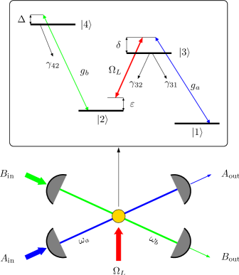
Figure 1: (Color online) A single four-level atom interacts with two cavity modes and a classical laser field. $A_{\text{in}}$ and $B_{\text{in}}$ are coherent input fields that drive the corresponding cavity resonantly, and $A_{\text{out}}$, $B_{\text{out}}$ are the output fields. The inset shows the atomic level scheme. The laser field with frequency $\omega_{\text{L}}$ and Rabi frequency $\Omega_{\text{L}}$ couples to the $|2\rangle\leftrightarrow|3\rangle$ transition, and the cavity mode with frequency $\omega_{a}$ interacts with the $|3\rangle\leftrightarrow|1\rangle$ transition. The second cavity mode with frequency $\omega_{b}$ interacts with the $|4\rangle\leftrightarrow|2\rangle$ transition. $g_{a}$ and $g_{b}$ are the single-photon Rabi frequencies corresponding to mode $a$ and $b$, respectively. The parameters $\gamma_{ij}$ are the decay rates of the various transitions, $\delta$ and $\Delta$ label the detuning of the cavity fields with transition $|3\rangle\leftrightarrow|1\rangle$ and $|4\rangle\leftrightarrow|2\rangle$, respectively, and $\varepsilon$ is the two-photon detuning.

We consider a single four-level atom that interacts with two cavity modes and a classical laser field, see Fig. 1. It was shown theoretically schmidt:96 and experimentally kang:03 that the considered level scheme can give rise to a strongly enhanced Kerr nonlinearity. In addition, this level configuration allows one to engineer a two-photon absorption process harris:98 ; kiffner:10b . Note that we chose the two-cavity setup in Fig. 1 because it allows us to present our model in a clear and unambiguous way. However, our setup could very well be realised with a single cavity where the two modes can be either two different polarisation or frequency modes. In particular, the two modes could have the same frequency and orthogonal polarisations.

The aim of this section is to derive an equation of motion for the reduced density operator $\varrho_{\text{F}}$ of the two cavity modes. We begin with a detailed description of the system shown in Fig. 1. The input field $A_{\text{in}}$ ($B_{\text{in}}$) is a coherent field that resonantly drives the cavity mode with frequency $\omega_{a}$ ($\omega_{b}$). The corresponding Hamiltonian is

$$H_{\text{in}}=\hbar\Omega_{a}^{*}e^{i\omega_{a}t}a+\hbar\Omega_{b}^{*}e^{i\omega_{b}t}b+\text{H.c.},$$ (1)

where H.c. stands for the Hermitian conjugate, and $a$ $(b)$ is the annihilation operator of the cavity mode with frequency $\omega_{a}$ ($\omega_{b}$). The Rabi frequencies $\Omega_{a}$ and $\Omega_{b}$ are determined by the input power of the fields $A_{\text{in}}$ and $B_{\text{in}}$, respectively. The cavity mode with frequency $\omega_{a}$ couples to the atomic transition $|3\rangle\leftrightarrow|1\rangle$, and the mode with frequency $\omega_{b}$ interacts with the atom on the $|4\rangle\leftrightarrow|2\rangle$ transition. In rotating-wave approximation (RWA), the interaction of the atom with the cavity modes is described by the Hamiltonian

$$H_{\text{C}}=-\hbar g_{a}a|3\rangle\langle 1|-\hbar g_{b}b|4\rangle\langle 2|+\text{H.c.},$$ (2)

where $g_{a}$ ($g_{b}$) is the single-photon Rabi frequency on the $|3\rangle\leftrightarrow|1\rangle$ ($|3\rangle\leftrightarrow|2\rangle$) transition. The detuning of the first cavity mode with the $|3\rangle\leftrightarrow|1\rangle$ transition is denoted by $\delta$, and $\Delta$ is the detuning of the second mode with the $|4\rangle\leftrightarrow|2\rangle$ transition,

$$\delta=\omega_{a}-\omega_{31}\,,\qquad\Delta=\omega_{b}-\omega_{42}\,.$$ (3)

The resonance frequencies on the $|3\rangle\leftrightarrow|1\rangle$ and $|4\rangle\leftrightarrow|2\rangle$ transitions have been labelled by $\omega_{31}$ and $\omega_{42}$, respectively. In addition, the atom interacts with a classical laser field with frequency $\omega_{\text{L}}$ and Rabi frequency $\Omega_{\text{L}}$, and this field couples to the $|3\rangle\leftrightarrow|2\rangle$ transition. In rotating-wave approximation, the atom-laser interaction reads

$$H_{\text{L}}=-\hbar\Omega_{\text{L}}|3\rangle\langle 2|e^{-i\omega_{\text{L}}t}+\text{H.c.}.$$ (4)

The free time evolution of the cavity modes and of the atomic degrees of freedom is given by $H_{\text{F}}$ and $H_{\text{A}}$, respectively,

$$H_{\text{F}}=\hbar\omega_{a}a^{\dagger}a+\hbar\omega_{b}b^{\dagger}b,$$ (5)

$$H_{\text{A}}=\hbar[\omega_{2}|2\rangle\langle 2|+\omega_{3}|3\rangle\langle 3|+\omega_{4}|4\rangle\langle 4|],$$ (6)

and we set $\omega_{1}=0$ in Eq. (6). With these definitions, we arrive at the master equation for the combined system of the atomic degrees of freedom and the two cavity modes,

$$\dot{\varrho}=-\frac{i}{\hbar}[H_{\text{F}}+H_{\text{in}}+H_{\text{A}}+H_{\text{L}}+H_{\text{C}},\varrho]+\mathcal{L}_{\gamma}\varrho+\mathcal{L}_{\kappa}\varrho\,.$$ (7)

The term $\mathcal{L}_{\gamma}\varrho$ in Eq. (7) describes spontaneous emission of the atom and is given by

$$\mathcal{L}_{\gamma}\varrho= -\frac{\gamma_{31}}{2}\left(S_{1}^{+}S_{1}^{-}\varrho+\varrho S_{1}^{+}S_{1}^{-}-2S_{1}^{-}\varrho S_{1}^{+}\right)$$

$$-\frac{\gamma_{32}}{2}\left(S_{2}^{+}S_{2}^{-}\varrho+\varrho S_{2}^{+}S_{2}^{-}-2S_{2}^{-}\varrho S_{2}^{+}\right)$$

$$-\frac{\gamma_{42}}{2}\left(S_{3}^{+}S_{3}^{-}\varrho+\varrho S_{3}^{+}S_{3}^{-}-2S_{3}^{-}\varrho S_{3}^{+}\right),$$ (8)

where $\gamma_{ij}$ is the full decay rate on the transition $|i\rangle\leftrightarrow|j\rangle$ (see Fig. 1). The atomic transition operators are defined as

$$S_{1}^{+}=|3\rangle\langle 1|,\quad S_{2}^{+}=|3\rangle\langle 2|,\quad S_{3}^{+}=|4\rangle\langle 2|,$$ (9)

and $S_{i}^{-}=(S_{i}^{+})^{\dagger}$. The last term $\mathcal{L}_{\kappa}\varrho$ in Eq. (7) accounts for photon losses at the cavity mirrors and reads

$$\mathcal{L}_{\kappa}\varrho= -\frac{\kappa_{a}}{2}(a^{\dagger}a\varrho+\varrho a^{\dagger}a-2a\varrho a^{\dagger})$$

$$-\frac{\kappa_{b}}{2}(b^{\dagger}b\varrho+\varrho b^{\dagger}b-2b\varrho b^{\dagger}),$$ (10)

where $\kappa_{a}$ ($\kappa_{b}$) is the damping rate of mode $a$ ($b$).

In appendix A, we derive from Eq. (7) the master equation for the reduced density operator $\varrho_{\text{F}}$ of the cavity modes alone,

$$\varrho_{\text{F}}=\text{Tr}_{\text{A}}\varrho=\varrho_{11}+\varrho_{22}+\varrho_{33}+\varrho_{44}\,,$$ (11)

and $\varrho_{\nu\nu}$ denotes $\langle\nu|\varrho|\nu\rangle$. If the two-photon detuning $\varepsilon=\omega_{a}-\omega_{\text{L}}-\omega_{2}$ vanishes, the master equation for the density operator $\tilde{\varrho}_{\text{F}}$ of the cavity modes in an interaction picture with respect to $H_{\text{F}}$ in Eq. (5) is given by

$$\dot{\tilde{\varrho}}_{\text{F}}=\mathcal{L}_{\text{in}}\tilde{\varrho}_{\text{F}}+\mathcal{L}_{\kappa}\tilde{\varrho}_{\text{F}}+\mathcal{L}_{U}\tilde{\varrho}_{\text{F}}+\mathcal{L}_{\Gamma}\tilde{\varrho}_{\text{F}},$$ (12)

where

$$\mathcal{L}_{\text{in}}\tilde{\varrho}_{\text{F}}=-i[\Omega_{a}^{*}a+\Omega_{b}^{*}b+\Omega_{a}a^{\dagger}+\Omega_{b}b^{\dagger},\tilde{\varrho}_{\text{F}}]$$ (13)

accounts for the coherent driving of the cavity modes and the cavity decay term $\mathcal{L}_{\kappa}\tilde{\varrho}_{\text{F}}$ is defined in Eq. (10). The two terms $\mathcal{L}_{U}\tilde{\varrho}_{\text{F}}$ and $\mathcal{L}_{\Gamma}\tilde{\varrho}_{\text{F}}$ in Eq. (12) represent the influence of the single atom on the evolution of the two cavity modes. More specifically,

$$\mathcal{L}_{U}\tilde{\varrho}_{\text{F}}=-i\,U[(ba)^{\dagger}ba,\tilde{\varrho}_{\text{F}}]$$ (14)

describes a coherent two-particle interaction between photons in modes $a$ and $b$. The strength of this interaction is determined via the parameter

$$U=\frac{|g_{a}|^{2}|g_{b}|^{2}}{(\Delta^{2}+\gamma_{42}^{2}/4)|\Omega_{\text{L}}|^{2}}\Delta.$$ (15)

Note that the sign of $U$ depends on the sign of the detuning $\Delta$ defined in Eq. (3). It follows that the interaction described by $\mathcal{L}_{U}$ can be repulsive or attractive. The last term in Eq. (12) is given by

$$\mathcal{L}_{\Gamma}\tilde{\varrho}_{\text{F}}=-\frac{\Gamma}{2}\left[(ba)^{\dagger}ba\tilde{\varrho}_{\text{F}}+\tilde{\varrho}_{\text{F}}(ba)^{\dagger}ba-2ba\tilde{\varrho}_{\text{F}}(ba)^{\dagger}\right]$$ (16)

and represents a two-photon loss term with decay rate

$$\Gamma=\frac{|g_{a}|^{2}|g_{b}|^{2}}{(\Delta^{2}+\gamma_{42}^{2}/4)|\Omega_{\text{L}}|^{2}}\gamma_{42}.$$ (17)

The dissipator $\mathcal{L}_{\Gamma}$ gives rise to the emission of correlated photon pairs. In each elementary emission process, $\mathcal{L}_{\Gamma}$ removes one photon out of mode $a$ and one photon out of mode $b$. In the following, we focus on the quantum correlations between the cavity modes that are induced by the two-photon loss term $\mathcal{L}_{\Gamma}$. For the rest of this paper, we will thus consider the purely dissipative scenario where the conservative photon-photon interaction vanishes, i.e. $U=0$. This situation arises when mode $b$ is resonant with the $|4\rangle\leftrightarrow|2\rangle$ transition and thus $\Delta=0$.

Next we summarise the conditions for the validity of the reduced master equation (12). The adiabatic elimination of the atomic degrees of freedom requires that the atomic decay rates $\gamma_{ij}$ are large as compared to the other system parameters,

$$\gamma_{42},\gamma_{31},\gamma_{32}\gg\kappa_{a},\kappa_{b},\sqrt{N_{a}N_{b}}\Gamma,\Omega_{a},\Omega_{b},|\delta|,$$ (18)

where $N_{a}$ ($N_{b}$) is the largest relevant photon number in mode $a$ ($b$). The master equation (12) for the cavity modes holds under the assumption that the two-photon detuning $\varepsilon$ vanishes. Since $\varepsilon=0$ can be adjusted only within a certain accuracy, we establish conditions that ensure the validity of Eq. (12) for $\varepsilon\not=0$ in Appendix B. Finally, the restriction to terms up to third order in the expansion of the density operator (54) requires

$$\frac{N_{a}|g_{a}|^{2}}{|\Omega_{\text{L}}|^{2}}\ll 1,\frac{N_{b}|g_{b}|^{2}}{|\Omega_{\text{L}}|^{2}}\ll 1,$$ (19)

where $N_{a}$ ($N_{b}$) is the maximal photon number in mode $a$ ($b$).

III STEADY STATE ANALYSIS

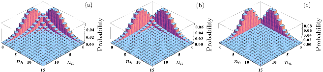
Figure 2: (Color online) Population of the cavity Fock states $|n_{a},n_{b}\rangle$ in steady state for (a) $\Omega_{a}=\Omega_{b}=1.32\times 10^{-2}\gamma_{42}$, $\kappa_{a}=\kappa_{b}=10^{-2}\gamma_{42}$, (b) $\Omega_{a}=\Omega_{b}=6.26\times 10^{-3}\gamma_{42}$, $\kappa_{a}=\kappa_{b}=0.5\times 10^{-2}\gamma_{42}$, and (c) $\Omega_{a}=\Omega_{b}=1.16\times 10^{-3}\gamma_{42}$, $\kappa_{a}=\kappa_{b}=10^{-3}\gamma_{42}$. The common parameters in (a)-(c) are $\Gamma=\gamma_{42}/100$, $\Delta=U=0$, $\delta=0$ and $\varepsilon=0$. The mean photon number for all states in (a)-(c) is $\langle\hat{N}\rangle=5$.

In this Section we characterise the steady state of the master equation (12) with a purely dissipative two-photon interaction ($\Delta=U=0$). Throughout this work we assume that the cavity decay rates $\kappa_{a}$ and $\kappa_{b}$ are different from zero. In this case and for time-independent input fields $\Omega_{a}$ and $\Omega_{b}$, the master equation (12) exhibits a unique steady state. If the two-photon decay term $\Gamma$ vanishes, this unique steady state is the pure state kraus:08 $\tilde{\varrho}_{\text{F}}=|\psi\rangle\langle\psi|$, where $|\psi\rangle=|\alpha_{a},\alpha_{b}\rangle$ and $|\alpha_{a}\rangle$ ($|\alpha_{b}\rangle$) denotes a coherent state in mode $a$ ($b$) with amplitude $\alpha_{a}=-2i\Omega_{a}/\kappa_{a}$ ($\alpha_{b}=-2i\Omega_{b}/\kappa_{b}$).

Next we turn to the general situation with $\Gamma\not=0$. In this case, the analytical steady state of the master equation (12) is difficult to obtain. A numerical study shows that the steady state of Eq. (12) is in general a mixed state. In addition, an intuitive understanding of the structure of this state can be gained via the dark states kraus:08 $|D\rangle$ of the two-photon loss term in Eq. (16) that obey $\mathcal{L}_{\Gamma}(|D\rangle\langle D|)=0$. Since $\mathcal{L}_{\Gamma}$ removes one photon out of each cavity mode in every elementary emission event, all pure dark states $|D\rangle$ must be of the form

$$|D\rangle=c_{1}|\phi_{a},0\rangle+c_{2}|0,\varphi_{b}\rangle,$$ (20)

where $|\phi_{a}\rangle$ and $|\varphi_{b}\rangle$ are arbitrary states (including the vacuum) of mode $a$ and $b$, respectively. Note that $\mathcal{L}_{\Gamma}$ supports an infinite number of dark states, and the most general dark state is given by a mixture of different pure dark states that are of the form of $|D\rangle$ in Eq. (20). In the regime where the two-photon decay rate $\Gamma$ dominates over the coherent drive terms $\Omega_{a}$, $\Omega_{b}$ and the cavity decay rates $\kappa_{1}$, $\kappa_{2}$, one can expect that the stationary state of Eq. (12) is approximately a dark state of $\mathcal{L}_{\Gamma}$ alone. This is confirmed by Fig. 2 that shows the population of the cavity Fock states $|n_{a},n_{b}\rangle$ in steady state for various parameters. These results were obtained via a numerical solution of Eq. (12). The relative importance of the two-photon loss term (16) is the smallest in Fig. 2(a) and the largest in Fig. 2(c). In the latter case it is apparent that the steady state is comprised of the dark states in Eq. (20). Only Fock states $|0,n_{b}\rangle$ and $|n_{a},0\rangle$ are significantly populated, while the population of other states $|n_{a},n_{b}\rangle$ with $n_{a}\not=0$ and $n_{b}\not=0$ is strongly suppressed. This result can be understood as follows. All Fock states $|n_{a},n_{b}\rangle$ with $n_{a}\not=0$ and $n_{b}\not=0$ experience not only the cavity loss term $\mathcal{L}_{\kappa}$, but the additional (strong) two-particle losses $\mathcal{L}_{\Gamma}$. This suppresses the population of these states via the cavity input fields.

The cavity pump fields $\Omega_{a}$, $\Omega_{b}$ induce transitions between dark states $|n_{a},0\rangle$, $|0,n_{b}\rangle$ and neighbouring Fock states $|n_{a},1\rangle$, $|1,n_{b}\rangle$ ($n_{a}\not=0$ and $n_{b}\not=0$). The latter states are not dark states of $\mathcal{L}_{\Gamma}$ and thus decay rapidly. However, we point out that this mechanism does not induce an indirect decay of the dark states $|0,n_{b}\rangle$, $|n_{a},0\rangle$ if $\Gamma$ becomes much larger than all other system parameters. The reason is that the transitions $|0,n_{b}\rangle\rightarrow|1,n_{b}\rangle\rightarrow|0,n_{b}-1\rangle$ ($|n_{a},0\rangle\rightarrow|n_{a},1\rangle\rightarrow|n_{a}-1,0\rangle$) occur at an effective rate comment1 $\Omega_{a}^{2}/\Gamma\ll 1$ ($\Omega_{b}^{2}/\Gamma\ll 1$) for $\Omega_{a}\ll\Gamma$ ($\Omega_{b}\ll\Gamma$) and are therefore negligible. This result can be regarded as a manifestation of the quantum Zeno effect ripoll:08 and explains the sharp population contrast between dark states $|n_{a},0\rangle$, $|0,n_{b}\rangle$ and neighbouring Fock states $|n_{a},1\rangle$, $|1,n_{b}\rangle$ in Fig. 2(c).

The most general pure dark state in Eq. (20) is a coherent superposition of the states $|\phi_{a},0\rangle$ and $|0,\varphi_{b}\rangle$. This is a remarkable feature since it implies that all strongly entangled NOON states

$$|\text{NOON}\rangle=\frac{1}{\sqrt{2}}(|N,0\rangle+|0,N\rangle)$$ (21)

and coherent superpositions thereof are dark states of the dissipator $\mathcal{L}_{\Gamma}$. Next we investigate whether the steady state of Eq. (12) contains entangled dark states or just a mixture of the states $|\phi_{a},0\rangle$ and $|0,\varphi_{b}\rangle$. Note that this information is not contained in Fig. 2 because it does not contain any information about the off-diagonal matrix elements of the density operator. We find that the steady state exhibits non-vanishing coherences in the Fock basis if the modes $a$ and $b$ appear in a completely symmetric fashion in the master equation (12). For example, for the parameters in Fig. 2(c), the diagonalisation of the numerically computed density operator shows that the steady state is very well approximated by a mixture of two coherent entangled states (CES),

$$\tilde{\varrho}_{\text{F}}\approx p_{1}|\text{CES}_{+}(\alpha_{1})\rangle\langle\text{CES}_{+}(\alpha_{1})|$$

$$+p_{2}|\text{CES}_{-}(\alpha_{2})\rangle\langle\text{CES}_{-}(\alpha_{2})|,$$ (22)

where $p_{1}\approx 0.499$, $p_{2}\approx 0.459$, $\alpha_{1}\approx-2.23i$, $\alpha_{2}\approx-2.29i$ and the CES states are defined as sanders:92 ; joo:11

$$|\text{CES}_{\pm}(\alpha)\rangle=\frac{1}{\sqrt{2(1\pm e^{-|\alpha|^{2}})}}(|\alpha,0\rangle\pm|0,\alpha\rangle).$$ (23)

The overlap between the approximate state in Eq. (22) and the full numerical solution in the trace norm is $95.44\%$.

Recently, the performance of CES in interferometric precision measurements was discussed in joo:11 . Since it was found that these states perform better than NOON states in a lossy interferometer, we discuss the suitability of the state in Eq. (22) for interferometric precision measurements. We find that the mixture in Eq. (22) performs approximately as good as classical light with a well-defined phase. Note, however, that the performance of a pure CES and the mixture in Eq. (22) differ only if the losses of the interferometer are smaller than approximately 25%. In this regime of a near-perfect interferometer, pure CES entangled states allow one to access the quantum regime that is currently inaccessible with our preparation method.

The previous discussion indicates that the steady state of the two cavity modes can be prepared in an entangled state. The entanglement properties of the cavity modes and of the output field are discussed in the following Sections IV and V, respectively.

IV ENTANGLEMENT OF THE CAVITY FIELD

The two modes of the cavity form a bipartite quantum system. By definition, the quantum state $\varrho_{\text{F}}$ of the cavity field is said to be entangled if and only if it is non-separable, and $\varrho_{\text{F}}$ is separable if and only if it can be written as

$$\varrho_{\text{F}}=\sum\limits_{j}p_{j}\varrho_{a}(j)\otimes\varrho_{b}(j)\,.$$ (24)

Here $\varrho_{a}(j)$ and $\varrho_{b}(j)$ are normalised states of the modes $a$ and $b$, respectively, and the parameters $p_{j}\geq 0$ are constrained by $\sum_{j}p_{j}=1$.

We employ two criteria that are both sufficient for the entanglement of the cavity modes. We begin with the Negativity vidal:02 that is defined as

$$\mathcal{N}(\varrho_{\text{F}})=\frac{1}{2}\left(1-\lVert\varrho_{\text{F}}^{\text{T}_{a}}\rVert_{1}\right),$$ (25)

where $\varrho_{\text{F}}^{\text{T}_{a}}$ denotes the partial transpose of $\varrho_{\text{F}}$ with respect to the subsystem $a$. The trace norm $\lVert A\rVert_{1}=\text{Tr}(\sqrt{A^{\dagger}A})$ of an operator $A$ is equal to the sum of its singular values. Note that the Negativity is an entanglement monotone, and hence $\mathcal{N}(\varrho_{\text{F}})>0$ is a sufficient criterion for the entanglement of the two field modes.

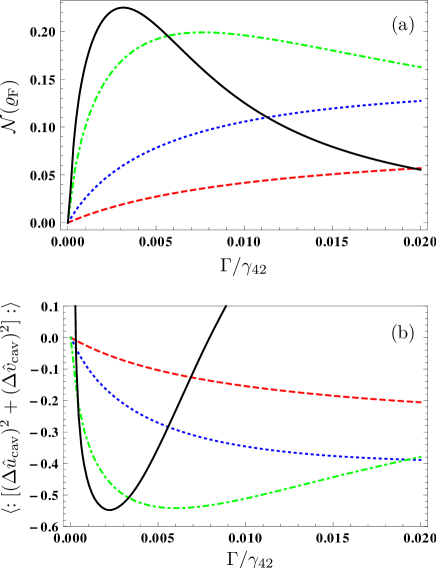
Figure 3: (Color online) Numerical evaluation of (a) the Negativity and (b) the inequality in Eq. (33) for the two cavity modes in steady state. The results are shown as a function of the two-particle loss rate $\Gamma$ and for different intensities of the coherent driving fields. The parameters are $\phi=\pi/2$, $\kappa_{a}=\kappa_{b}=10^{-2}\gamma_{42}$, $\Delta=U=0$, $\delta=0$ and $\varepsilon=0$. The red dashed line corresponds to $\Omega_{a}=\Omega_{b}=0.2\times 10^{-2}\gamma_{42}$, the blue dotted line stands for $\Omega_{a}=\Omega_{b}=0.4\times 10^{-2}\gamma_{42}$, the green dashed-dotted line corresponds to $\Omega_{a}=\Omega_{b}=1\times 10^{-2}\gamma_{42}$ and the black solid line stand for $\Omega_{a}=\Omega_{b}=1.6\times 10^{-2}\gamma_{42}$.

The second criterion is derived in duan:00 and states that the system is in an entangled quantum state if the total variance of two Einstein-Podolsky-Rosen (EPR) type operators $\hat{u}$ and $\hat{v}$ of the two modes satisfy the inequality

$$\langle\left(\delta\hat{u}_{\text{cav}}\right)^{2}+\left(\delta\hat{v}_{\text{cav}}\right)^{2}\rangle<2\,,$$ (26)

where

$$\hat{u}_{\text{cav}}=\hat{x}_{a}+\hat{x}_{b}\,,\qquad\hat{v}_{\text{cav}}=\hat{p}_{a}-\hat{p}_{b}\,.$$ (27)

For any operator $X$, we define $\delta\hat{X}=\hat{X}-\langle\hat{X}\rangle$, and $\hat{x}_{k}$ and $\hat{p}_{k}$ are local operators which correspond to mode $k\in\{a,b\}$ with frequency $\omega_{k}$. The only restriction imposed on the operators $\hat{x}_{k}$ and $\hat{p}_{k}$ is that they must obey the commutation relation

$$[\hat{x}_{k},\hat{p}_{l}]=i\delta_{kl}\,,$$ (28)

but are otherwise arbitrary. Here we choose for $\hat{x}_{k}$ and $\hat{p}_{l}$ the quadrature operators of the cavity fields

$$\hat{x}_{a}=\frac{1}{\sqrt{2}}(\tilde{a}e^{-i\phi}+\tilde{a}^{\dagger}e^{i\phi}),$$ (29)

$$\hat{p}_{a}=\frac{1}{\sqrt{2}i}(\tilde{a}e^{-i\phi}-\tilde{a}_{k}^{\dagger}e^{i\phi}),$$ (30)

$$\hat{x}_{b}=\frac{1}{\sqrt{2}}(\tilde{b}e^{-i\phi}+\tilde{b}^{\dagger}e^{i\phi}),$$ (31)

$$\hat{p}_{b}=\frac{1}{\sqrt{2}i}(\tilde{b}e^{-i\phi}-\tilde{b}_{k}^{\dagger}e^{i\phi}),$$ (32)

where $\tilde{a}=e^{i\omega_{a}t}a$ and $\tilde{b}=e^{i\omega_{b}t}b$ are slowly varying in time. Since $\hat{u}_{\text{cav}}$ and $\hat{v}_{\text{cav}}$ can be identified with the operators corresponding to the centre-of-mass motion and the relative momentum of two quantum mechanical oscillators, respectively, they are called EPR type operators. The phase $\phi$ is arbitrary and will be optimised such that a maximal violation of the inequality (26) is achieved.

The inequality in Eq. (26) is equivalent to

$$\langle:[\left(\delta\hat{u}_{\text{cav}}\right)^{2}+\left(\delta\hat{v}_{\text{cav}}\right)^{2}]:\rangle<0\,,$$ (33)

where $:\ :$ denotes normal ordering (all creation operators to the left) with respect to the operators $a$, $b$ and their adjoints. For reasons that will become clear later (see Sec. V), we will employ Eq. (33) instead of Eq. (26). With the help of Eqs. (27) and (29)-(32), we find

$$\langle:[(\delta\hat{u}_{\text{cav}})^{2}+(\delta\hat{v}_{\text{cav}})^{2}]:\rangle=2\big{[}\langle\delta\tilde{a}^{\dagger}\delta\tilde{a}\rangle$$

$$\hskip 28.45274pt+\langle\delta\tilde{b}^{\dagger}\delta\tilde{b}\rangle+\langle\delta\tilde{a}\delta\tilde{b}\rangle e^{-2i\phi}+\langle\delta\tilde{a}^{\dagger}\delta\tilde{b}^{\dagger}\rangle e^{2i\phi}\big{]}.$$ (34)

We numerically solve for the steady state of the density operator of the two cavity modes via the master equation (12) for various parameters $\Gamma$ and different intensities of the coherent input fields. The result for the entanglement criteria in Eqs. (25) and (34) is shown in Figs. 3(a) and (b), respectively. It follows that the steady state of the system exhibits entanglement. The Negativity and the normally ordered variance of the EPR-type operators show a qualitatively similar (but mirrored) behaviour in the weak driving regime. A different situation arises if the Rabi frequencies $\Omega_{a}$ and $\Omega_{b}$ become comparable to the cavity decay rates. Although the cavity modes are entangled for all parameters in Fig. 3(a) (the Negativity is larger than zero), the sufficient entanglement criterion in Eq. (33) is not fulfilled for larger values of $\Gamma/\gamma_{42}$. We show in Sec. V and Appendix C that the quantity in Eq. (34) and hence the entanglement criterion in Eq. (33) can be measured experimentally. The discussion above shows that this approach allows one to capture the entanglement for a large range of parameters, but it fails to detect the entanglement in some cases.

V ENTANGLEMENT OF THE OUTPUT FIELD

The output field of the cavity is a multi-mode field. The question whether the output field is entangled thus requires to specify the corresponding modes. In standard input-output theory gardiner:85 ; clerk:10 , the output fields $A_{\text{out}}$ and $B_{\text{out}}$ [see Fig. 1] are defined as

$$A_{\text{out}}(t)=\frac{1}{\sqrt{2\pi}}\int\text{d}\omega e^{-i\omega(t-t_{1})}A(\omega,t_{1}),$$ (35)

$$B_{\text{out}}(t)=\frac{1}{\sqrt{2\pi}}\int\text{d}\omega e^{-i\omega(t-t_{1})}B(\omega,t_{1}).$$ (36)

Here $A(\omega,t_{1})$ and $B(\omega,t_{1})$ are the Heisenberg operators of the continuous output modes taken at time $t_{1}\rightarrow\infty$. The latter operators obey the equal-time commutation relations

$$[A(\omega,t),A^{\dagger}(\omega^{\prime},t)]=[B(\omega,t),B^{\dagger}(\omega^{\prime},t)]=\delta(\omega-\omega^{\prime}).$$ (37)

Here we focus on the entanglement between two modes corresponding to the central frequencies $\omega_{a}$ and $\omega_{b}$ of $A_{\text{out}}$ and $B_{\text{out}}$, respectively. Our aim is to follow a similar approach as in Eq. (33) where we employ the variance of EPR-type operators as a sufficient criterion for entanglement duan:00 . Therefore, we have to define position- and momentum-like operators that obey the canonical commutation relation (28). In order to achieve this, we have to construct a discrete mode of $A_{\text{out}}$ from the continuous mode operator $A(\omega,t_{1})$. This transition can be achieved if we average $A(\omega,t_{1})$ over a small frequency interval $\Delta\omega$ centered at $\omega_{a}$,

$$\mathcal{A}_{0}= \frac{1}{\sqrt{\Delta\omega}}\int\limits_{-\Delta\omega/2}^{\Delta\omega/2}\text{d}\omega e^{i(\omega_{a}+\omega)t_{1}}A(\omega_{a}+\omega,t_{1}),$$ (38)

$$= \frac{1}{\sqrt{2\pi\Delta\omega}}\int\limits_{-\Delta\omega/2}^{\Delta\omega/2}\text{d}\omega\int\limits_{-\infty}^{\infty}\text{d}t\tilde{A}_{\text{out}}(t)e^{i\omega t},$$

where the output field $\tilde{A}_{\text{out}}(t)=e^{i\omega_{a}t}A_{\text{out}}(t)$ is slowly varying in time. Similarly, we define a discrete mode of the output field $B_{\text{out}}$ centered at $\omega_{b}$,

$$\mathcal{B}_{0}= \frac{1}{\sqrt{2\pi\Delta\omega}}\int\limits_{-\Delta\omega/2}^{\Delta\omega/2}\text{d}\omega\int\limits_{-\infty}^{\infty}\text{d}t\tilde{B}_{\text{out}}(t)e^{i\omega t},$$ (39)

and $\tilde{B}_{\text{out}}(t)=e^{i\omega_{b}t}B_{\text{out}}(t)$. The modes $\mathcal{A}_{0}$ and $\mathcal{B}_{0}$ represent modes of the output fields $A_{\text{out}}$ and $B_{\text{out}}$ that are experimentally accessible via spectral filtering. Furthermore, we note that $\langle\mathcal{A}_{0}^{\dagger}\mathcal{A}_{0}\rangle$ can be interpreted agarwal:qst2 as the mean number of photons emitted into the mode $\mathcal{A}_{0}$ within the time $1/\Delta\omega$ (the same statement holds for the mode $\mathcal{B}_{0}$).

Since the two discrete modes $\mathcal{A}_{0}$ and $\mathcal{B}_{0}$ obey the commutation relations

$$[\mathcal{A}_{0},\mathcal{A}_{0}^{\dagger}]=[\mathcal{B}_{0},\mathcal{B}_{0}^{\dagger}]=1,\quad[\mathcal{A}_{0},\mathcal{B}_{0}^{\dagger}]=[\mathcal{A}_{0},\mathcal{B}_{0}]=0,$$ (40)

we can define position- and momentum-like operators for each mode that obey the canonical commutation relation (28),

$$\hat{x}_{\mathcal{A}}=\frac{1}{\sqrt{2}}(\mathcal{A}_{0}e^{-i\phi}+\mathcal{A}_{0}^{\dagger}e^{i\phi}),$$ (41)

$$\hat{p}_{\mathcal{A}}=\frac{1}{\sqrt{2}i}(\mathcal{A}_{0}e^{-i\phi}-\tilde{A}_{0}^{\dagger}e^{i\phi})$$ (42)

$$\hat{x}_{\mathcal{B}}=\frac{1}{\sqrt{2}}(\mathcal{B}_{0}e^{-i\phi}+\mathcal{B}_{0}^{\dagger}e^{i\phi}),$$ (43)

$$\hat{p}_{\mathcal{B}}=\frac{1}{\sqrt{2}i}(\mathcal{B}_{0}e^{-i\phi}-\mathcal{B}_{0}^{\dagger}e^{i\phi}).$$ (44)

The phase $\phi$ in Eqs. (41) and (44) is arbitrary and later on chosen such that the necessary separability condition is maximally violated. We can now proceed as in Sec. IV and define EPR-type operators

$$\hat{u}_{0}=\hat{x}_{\mathcal{A}}+\hat{x}_{\mathcal{B}}\,,\qquad\hat{v}_{0}=\hat{p}_{\mathcal{A}}-\hat{p}_{\mathcal{B}}\,.$$ (45)

With the help of Eqs. (45) and (41)-(44), we find that the normally ordered total variance of the operators $\hat{u}_{0}$ and $\hat{v}_{0}$ is given by

$$\langle:[(\delta\hat{u}_{0})^{2}+(\delta\hat{v}_{0})^{2}]:\rangle=\frac{1}{\Delta\omega}\int\limits_{-\Delta\omega/2}^{\Delta\omega/2}\text{d}\omega[S_{u}(\omega)+S_{v}(\omega)],$$ (46)

where $S_{u}(\omega)$ and $S_{v}(\omega)$ are related to the two-mode squeezing spectra of the output fields. A definition of these functions and how they can be calculated numerically and measured experimentally is provided in Appendix C.

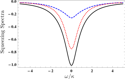
Figure 4: (Color online) Squeezing spectra. The blue dashed line corresponds to $S_{u}(\omega)$, the red dotted line to $S_{v}(\omega)$ and the black solid line shows $S_{u}(\omega)+S_{v}(\omega)$. The parameters are $\phi=\pi/2$, $\kappa=\kappa_{a}=\kappa_{b}=10^{-2}\gamma_{42}$, $\Gamma=\gamma_{42}/100$, $\Omega_{a}=\Omega_{b}=0.7\times 10^{-2}\gamma_{42}$, $\Delta=U=0$, $\delta=0$ and $\varepsilon=0$.

According to the entanglement criterion in duan:00 , the modes $\mathcal{A}_{0}$ and $\mathcal{B}_{0}$ are entangled if the left-hand side of Eq. (46) is smaller than zero. If $\Delta\omega$ is sufficiently small, this means that modes $\mathcal{A}_{0}$ and $\mathcal{B}_{0}$ are entangled if $S_{u}(0)+S_{v}(0)<0$. The numerical evaluation of the squeezing spectra $S_{u}$ and $S_{v}$ in Fig. 4 demonstrates clearly the entanglement of the output modes. For the chosen parameters, we find a two-mode squeezing of $-1.3\text{dB}$ in $S_{u}$ and $-6.1\text{dB}$ in $S_{v}$ at the central frequency $\omega=0$.

So far we considered the entanglement between the two central frequency components at $\omega_{a}$ and $\omega_{b}$. Note that our approach can be generalised to modes centered around $\omega_{a}-\omega$ and $\omega_{b}+\omega$ if the output spectra of modes $a$ and $b$ are completely symmetric and if the two modes are interchangeable in the master equation (12). In previous works braunstein:05 ; morigi:06 ; morigi2:06 , other EPR-type operators than those in Eqs. (45) with (41)-(44) were defined, and their variances can also be related to squeezing spectra. However, in the latter approach it is not obvious to identify the modes of the output field that are entangled.

Finally, we address the experimental verification of the entanglement inside the cavity. To this end, we note that

$$\frac{1}{\kappa}\int\limits_{-\infty}^{\infty}\text{d}\omega[S_{u}(\omega)+S_{v}(\omega)]=\langle:[(\delta\hat{u}_{\text{cav}})^{2}+(\delta\hat{v}_{\text{cav}})^{2}]:\rangle,$$ (47)

and hence it follows that the field inside the cavity is entangled if the sum of $S_{u}(\omega)+S_{v}(\omega)$, integrated over all frequencies, is negative [see Eq. (33)]. Note that the variance of the cavity fields can be measured directly without recording the squeezing spectra jing:06 .

VI EXPERIMENTAL REALIZATION

Next we discuss the experimental implementation of our scheme in Fig. 1. A key requirement of our scheme is that the single atom should have a very well defined position that changes very little over the range of an optical wavelength. Ideal candidates are therefore single trapped neutral atoms weber:09 ; khudaverdyan:09 or ions stute:11a ; russo:09 ; mundt:03 ; keller:04 ; devoe:96 inside an optical cavity. Recently, several experiments with ${}^{40}\text{Ca}^{+}$ ions inside a high-finesse optical cavity have been reported stute:11a ; russo:09 ; mundt:03 ; keller:04 . A suitable candidate would also be given by a ${}^{138}\text{Ba}^{+}$ ion devoe:96 , where the level scheme in Fig. 1 could be realised between two $J=1/2$ Zeeman manifolds via polarisation- and frequency selection. Alternatively, the level scheme in Fig. 1 can be realised with artificial atoms rebic:09 coupled to microwave fields.

In our approach we obtain an effective, engineered master equation for the cavity modes alone via an adiabatic elimination of the atomic degrees of freedom. In particular, this requires that that the cavity decay rates are much smaller than the atomic spontaneous emission decay rates, see Eq. (18). In a recent experiment stute:11a ; russo:09 with a ${}^{40}\text{Ca}^{+}$ ion in a high-finesse cavity, the ratio between the atomic decay rate and the corresponding cavity decay rate is $\gamma/\kappa\approx 16$. At the same time, the coupling constant $g$ was larger than the atomic decay rate, $g/\gamma\approx 2$ stute:11a . However, we show in appendix D that it is advantageous to realise our scheme with $g/\gamma<1$. This opens up the possibility to increase the length $L$ of the cavity which will reduce the magnitudes of the coupling constant $|g|\sim 1/\sqrt{L}$ and of the cavity decay rate $\kappa\sim 1/L$. From the above example, we conclude that values of $\gamma/\kappa\approx 100$ should be achievable with current technology. Valid choices for the remaining system parameters that comply with the conditions (18) and (19) of our model are discussed in appendix D. In summary, an increase in the number of photons in the cavity requires a reduction in the two-photon decay rate $\Gamma$. Note that this does not necessarily result in a smaller entanglement between the cavity modes. On the contrary, Fig. 3 indicates that the maximal entanglement is attained for smaller two-photon decay rates $\Gamma$ if the number of photons increases (see Sec. IV).

VII SUMMARY AND OUTLOOK

This paper investigates a scheme for dissipative quantum state preparation for two optical cavity modes $a$ and $b$. We engineer an effective reservoir via a single, laser-driven four level atom that interacts with both cavity modes on separate transitions. The adiabatic elimination of the atomic degrees of freedom gives rise to a master equation for the cavity modes alone and contains a two-photon loss term. Each elementary emission event induced by this two-photon loss term removes one photon out of mode $a$ and one photon out of mode $b$. We find that the dark states of this loss term are given by all entangled NOON states and superpositions thereof. If the two cavity modes are interchangeable in the corresponding master equation, the steady state of the cavity field exhibits entanglement. We employ the Negativity as well as an inequality duan:00 based on Einstein-Podolsky-Rosen type observables as sufficient entanglement criteria. While the former is an entanglement monotone, the latter can be measured via two balanced homodyne detection setups of the output fields. Furthermore, we define suitable modes of the output fields and show that they can be entangled as well. The entanglement of the output modes can be verified experimentally via the measurement of two-mode squeezing spectra.

The stationary state inside the cavity can be well approximated by a mixture of two CES states for specific parameters. While a pure CES state is able to access the quantum regime in interferometric precision measurements with small photon losses inside the interferometer, the mixture prepared by our dissipative scheme does not perform better than classical light with a well defined phase. However, modifications of our scheme may pave the way towards the dissipative preparation of NOON states and CES that are relevant for quantum-enhanced technologies. In the ideal case, it may help to prepare photon states that allow one to achieve the ultimate quantum limit escher:11 in interferometric precision measurements with realistic photon losses.

Appendix A Derivation of the reduced master equation

Here we outline the derivation of the effective master equation for the cavity modes in Eq. (12). The starting point for our derivation is the full master equation in Eq. (7). Next we apply a unitary transformation $W=W_{\text{F}}\otimes W_{\text{A}}$ to Eq. (7), where $W_{\text{F}}=\exp[iH_{\text{F}}t/\hbar]$ acts only on the cavity modes, and

$$W_{\text{A}}= \exp[i(H_{\text{A}}/\hbar+\varepsilon|2\rangle\langle 2|+\delta|3\rangle\langle 3|+(\Delta+\varepsilon)|4\rangle\langle 4|)t]$$ (48)

acts only on the atomic degrees of freedom. The density operator in the new frame is denoted by $\tilde{\varrho}=W\varrho W^{\dagger}$ and obeys the equation of motion

$$\dot{\tilde{\varrho}}=-\frac{i}{\hbar}[H_{0}+H_{\text{C}},\tilde{\varrho}]+\mathcal{L}_{\gamma}\tilde{\varrho}+\mathcal{L}_{\text{IO}}\tilde{\varrho}\,,$$ (49)

where

$$H_{0}=-\hbar[ \varepsilon|2\rangle\langle 2|+\delta|3\rangle\langle 3|+(\Delta+\varepsilon)|4\rangle\langle 4|$$

$$+\Omega_{\text{L}}|3\rangle\langle 2|+\Omega_{\text{L}}^{*}|2\rangle\langle 3|],$$ (50)

and $\varepsilon=\omega_{a}-\omega_{\text{L}}-\omega_{2}$ is the two-photon detuning. The super-operator $\mathcal{L}_{\text{IO}}=\mathcal{L}_{\text{in}}+\mathcal{L}_{\kappa}$ in Eq. (49) accounts for the external driving via the input fields and the damping of the cavity modes, where $\mathcal{L}_{\text{in}}$ and $\mathcal{L}_{\kappa}$ are defined in Eqs. (13) and (10), respectively. The master equation for the transformed density operator $\tilde{\varrho}_{\text{F}}$ of the cavity modes is obtained if we trace over the atomic degrees of freedom in Eq. (49),

$$\dot{\tilde{\varrho}}_{\text{F}}=\left(ig_{a}^{*}[a^{\dagger},\tilde{\varrho}_{31}]+ig_{b}^{*}[b^{\dagger},\tilde{\varrho}_{42}]+\text{H.c.}\right)+\mathcal{L}_{\text{IO}}\tilde{\varrho}_{\text{F}}.$$ (51)

In order to eliminate the coherences $\tilde{\varrho}_{31}$ and $\tilde{\varrho}_{42}$ from Eq. (51), we solve Eq. (49) perturbatively in the Hamiltonian $H_{\text{C}}$ describing the interaction between the atom and the cavity modes. In order to obtain the desired expansion of the full density operator $\tilde{\varrho}$ in the coupling constants $g_{a}$ and $g_{b}$, we re-write Eq. (49) in a form where the atom-cavity interaction is separated from the other terms,

$$\dot{\tilde{\varrho}}=\mathcal{L}_{0}\tilde{\varrho}-\frac{i}{\hbar}[H_{\text{C}},\tilde{\varrho}],$$ (52)

and the super-operator $\mathcal{L}_{0}$ is defined by

$$\mathcal{L}_{0}\tilde{\varrho}=-\frac{i}{\hbar}[H_{0},\tilde{\varrho}]+\mathcal{L}_{\gamma}\tilde{\varrho}+\mathcal{L}_{\text{IO}}\tilde{\varrho}.$$ (53)

Expansion of the density operator in Eq. (52) as

$$\tilde{\varrho}=\sum\limits_{k=0}^{\infty}\tilde{\varrho}^{(k)},$$ (54)

where $\tilde{\varrho}^{(k)}$ denotes the contribution to $\tilde{\varrho}$ in $k$th order in $H_{\text{C}}$, leads to the following set of coupled differential equations

$$\dot{\tilde{\varrho}}^{(0)}=\mathcal{L}_{0}\tilde{\varrho}^{(0)}\,,$$ (55)

$$\dot{\tilde{\varrho}}^{(k)}=\mathcal{L}_{0}\tilde{\varrho}^{(k)}-\frac{i}{\hbar}[H_{\text{C}},\tilde{\varrho}^{(k-1)}],\quad k>0.$$ (56)

Equation (55) describes the interaction of the atom with the classical laser fields to all orders and in the absence of the cavity fields. Higher-order contributions to $\tilde{\varrho}$ can be obtained if Eq. (56) is solved iteratively. Equations (55) and (56) must be solved under the constraints $\text{Tr}(\tilde{\varrho}^{(0)})=1$ and $\text{Tr}(\tilde{\varrho}^{(k)})=0$ ($k>0$). We employ a Markov-type approximation and assume that the atom reaches its steady state on a timescale that is fast as compared to the typical evolution time of $\tilde{\varrho}_{\text{F}}$ induced by the atom-cavity coupling. In addition, we suppose that the cavity decay rates $\kappa_{a}$, $\kappa_{b}$ and the Rabi frequencies $\Omega_{a}$, $\Omega_{b}$ are small as compared to the atomic decay rates $\gamma_{ij}$ and hence neglect the contribution of the super-operator $\mathcal{L}_{\text{IO}}$ to $\mathcal{L}_{0}$. Under these conditions, the set of equations (55) and (56) can be solved in a straightforward manner if $\mathcal{L}_{0}$ is represented by a matrix. However, the procedure is tedious since $H_{\text{C}}$ contains the operators $a$ and $b$, and hence one has to keep track of the operator ordering. Up to third order, $\tilde{\varrho}\approx\tilde{\varrho}^{(0)}+\tilde{\varrho}^{(1)}+\tilde{\varrho}^{(2)}+\tilde{\varrho}^{(3)}$, and for vanishing two-photon detuning $\varepsilon=0$ we find

$$\tilde{\varrho}_{31}=\mathcal{A}g_{a}|g_{b}|^{2}b^{\dagger}ba\tilde{\varrho}_{\text{F}},$$ (57)

$$\tilde{\varrho}_{42}=\mathcal{A}g_{b}|g_{a}|^{2}ba\tilde{\varrho}_{\text{F}}a^{\dagger},$$ (58)

where

$$\mathcal{A}=\frac{-1}{(\Delta+i\gamma_{42}/2)|\Omega_{\text{L}}|^{2}}.$$ (59)

Finally, we substitute Eqs. (57) and (58) in Eq. (51) and obtain the master equation (12).

Appendix B Finite two-photon detuning $\varepsilon\not=0$

Here we establish conditions that ensure the validity of Eq. (12) for non-zero two photon detuning. For simplicity we limit the discussion to the case of a purely dissipative photon-photon interaction ($U=\Delta=0$). In the ideal case $\varepsilon=0$, only the third-order term contributes to the coherences in Eqs. (57) and (58). The first-order term for $\varepsilon\not=0$ gives rise to an additional term $\mathcal{L}_{1}\varrho_{\text{F}}$ on the right-hand side of Eq. (12). Up to second order in $\varepsilon$, we find

$$\mathcal{L}_{1}\varrho_{\text{F}}= -\frac{i}{\hbar}[H_{1},\varrho_{\text{F}}]$$

$$-\frac{\Gamma_{1}}{2}(a^{\dagger}a\varrho_{\text{F}}+\varrho_{\text{F}}a^{\dagger}a-2a\varrho_{\text{F}}a^{\dagger}),$$ (60)

where

$$H_{1}=-\hbar|g_{a}|^{2}\frac{\delta\varepsilon^{2}+\varepsilon|\Omega_{\text{L}}|^{2}}{2|\Omega_{\text{L}}|^{4}}a^{\dagger}a$$ (61)

$$\Gamma_{1}=\gamma_{3}\frac{|g_{a}|^{2}}{|\Omega_{\text{L}}|^{4}}\varepsilon^{2},$$ (62)

and $\gamma_{3}=\gamma_{31}+\gamma_{32}$ is the full decay rate of state $|3\rangle$. Here $H_{1}$ is just a frequency shift of mode $a$, and the term proportional to $\Gamma_{1}$ describes an additional decay channel for photons in mode $a$. This term can be neglected provided that

$$\Gamma_{1}=\gamma_{3}\frac{|g_{a}|^{2}}{|\Omega_{\text{L}}|^{4}}\varepsilon^{2}\ll\kappa_{a}.$$ (63)

The second-order contribution $\tilde{\varrho}^{(2)}$ is equal to zero for all parameters. On the other hand, other third-order terms occur for $\varepsilon\not=0$ that give rise to other two-particle processes in Eq. (12). The magnitude of these terms relative to the terms proportional to $\Gamma$ in Eq. (12) is negligible provided that $|\varepsilon|,|\delta|\ll\gamma_{31},\gamma_{32},\gamma_{42}$ and

$$\frac{|\varepsilon|(\gamma_{3}+\gamma_{42})}{|\Omega_{\text{L}}|^{2}}\ll 1, \frac{|\delta\varepsilon|}{|\Omega_{\text{L}}|^{2}}\ll 1.$$ (64)

Appendix C Definition and measurement of squeezing spectra

The two-mode squeezing spectra are defined as

$$S_{u}(\omega)=2\int\limits_{0}^{\infty}\text{d}\tau\cos\omega\tau\langle\mathcal{T}:\delta\hat{u}_{\text{out}}(t+\tau)\delta\hat{u}_{\text{out}}(t):\rangle,$$ (65)

$$S_{v}(\omega)=2\int\limits_{0}^{\infty}\text{d}\tau\cos\omega\tau\langle\mathcal{T}:\delta\hat{v}_{\text{out}}(t+\tau)\delta\hat{v}_{\text{out}}(t):\rangle,$$ (66)

where

$$\hat{u}_{\text{out}}=\hat{x}_{A}+\hat{x}_{B},\qquad\hat{v}_{\text{out}}=\hat{p}_{A}-\hat{p}_{B},$$ (67)

and the quadratures of the output field are given by

$$\hat{x}_{A}=\frac{1}{\sqrt{2}}(\tilde{A}_{\text{out}}e^{-i\phi}+\tilde{A}_{\text{out}}^{\dagger}e^{i\phi}),$$ (68)

$$\hat{p}_{A}=\frac{1}{\sqrt{2}i}(\tilde{A}_{\text{out}}e^{-i\phi}-\tilde{A}_{\text{out}}^{\dagger}e^{i\phi})$$ (69)

$$\hat{x}_{B}=\frac{1}{\sqrt{2}}(\tilde{B}_{\text{out}}e^{-i\phi}+\tilde{B}_{\text{out}}^{\dagger}e^{i\phi}),$$ (70)

$$\hat{p}_{B}=\frac{1}{\sqrt{2}i}(\tilde{B}_{\text{out}}e^{-i\phi}-\tilde{B}_{\text{out}}^{\dagger}e^{i\phi}).$$ (71)

The operator $\mathcal{T}$ in Eq. (66) orders products of annihilation operators such that their time arguments increase from right to left, and products of creation operators are ordered such that time arguments increase from left to right. Since the definition of $S_{u}$ and $S_{v}$ comprises only expectation values of normally and time-ordered products of the output fields, we can easily represent $S_{u}$ and $S_{v}$ in terms of the cavity fields gardiner:85 ,

$$S_{u}(\omega)=2\kappa\int\limits_{0}^{\infty}\text{d}\tau\cos\omega\tau\langle\mathcal{T}:\delta\hat{u}_{\text{cav}}(t+\tau)\delta\hat{u}_{\text{cav}}(t):\rangle,$$ (72)

$$S_{v}(\omega)=2\kappa\int\limits_{0}^{\infty}\text{d}\tau\cos\omega\tau\langle\mathcal{T}:\delta\hat{v}_{\text{cav}}(t+\tau)\delta\hat{v}_{\text{cav}}(t):\rangle,$$ (73)

where $\hat{u}_{\text{cav}}$ and $\hat{v}_{\text{cav}}$ are defined in Eq. (27).

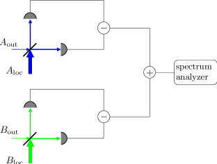
Figure 5: (Color online) Measurement of the two-mode squeezing spectrum $S_{u}(\omega)$ in Eq. (72). The output field $A_{\text{out}}$ ($B_{\text{out}}$) is superimposed with a strong coherent field at a $50:50$ beamsplitter, and the photocurrents of each detector are subtracted. The photocurrents of the two balanced homodyne detections are added and fed into a spectrum analyser. The resulting spectrum is given by Eq. (74) and directly proportional to $S_{u}(\omega)$.

The general setup for the measurement of the two-mode squeezing spectra morigi:06 ; morigi2:06 is shown in Fig. 5. The output field $A_{\text{out}}$ ($B_{\text{out}}$) is superimposed with a strong coherent field at a $50:50$ beamsplitter, and the photocurrents of each detector are subtracted. A similar measurement is performed for the output field $B_{\text{out}}$. The local oscillator fields are given by $A_{\text{loc}}=|\alpha|e^{i\theta}$ and $B_{\text{loc}}=|\beta|e^{i\theta}$, where $|\alpha|=|\beta|$ and the phase $\theta=\phi-\pi/2$ determines the phase $\phi$ occurring in the definition (69)-(71) of the quadrature operators. The photocurrents of the two balanced homodyne detections are added and the resulting current $i$ is fed into a spectrum analyser. The recorded spectrum is then given by mandel:qo

$$P_{u}(\omega)= \frac{1}{\pi}\int\limits_{0}^{\infty}\text{d}\tau\cos\omega\tau\lim\limits_{t\rightarrow\infty}[\langle i(t)i(t+\tau)\rangle-\langle i(t)\rangle^{2}]$$

$$=P_{\text{shot}}[1+\eta S_{u}(\omega)],$$ (74)

where $P_{\text{shot}}$ is the shot-noise limit and $\eta$ is the detection efficiency. The spectrum $S_{v}(\omega)$ can be measured with the same setup if the phases of the local oscillators are changed according to $\theta\rightarrow\theta+\pi/2$, and the photocurrents of the two homodyne detections have to be subtracted rather than added.

Appendix D Parameter choices

The validity of our approach requires that the conditions in Eqs. (18) and (19) are fulfilled. Here we discuss the possible choices for the system parameters that comply with these conditions. For simplicity, we assume that the coupling constants, cavity decay rates, Rabi frequencies and the Fock state cutoffs are identical for both modes. We thus set $|g_{a}|=|g_{b}|=|g|$, $\kappa_{1}=\kappa_{2}=\kappa$, $\Omega_{a}=\Omega_{b}=\Omega$ and $N_{a}=N_{b}=N$. Furthermore, all atomic decay rates are assumed to be the same, $\gamma=\gamma_{31}=\gamma_{32}=\gamma_{42}$, and we introduce dimensionless parameters $\tilde{p}=p/\gamma$ that are denoted by a tilde. Since we are only interested in the purely dissipative situation, we limit the discussion to the case $\Delta=0$ such that the conservative photon-photon interaction $U$ vanishes. We begin with the cutoff $N$ in the Fock state basis that is determined by the Rabi frequency $\tilde{\Omega}$ driving the cavity modes, the cavity decay rate $\tilde{\kappa}$ and the two-photon decay rate $\tilde{\Gamma}$. Note that Eq. (18) requires these parameters to be much smaller than unity, and thus $N$ cannot be arbitrarily large for realistic values of $\tilde{\kappa}$. Next we discuss the condition for the two-photon decay rate $\tilde{\Gamma}$ in Eq. (18) and the inequality in Eq. (19). For a given cutoff $N$ of the Fock state basis, these two conditions read

$$N\tilde{\Gamma}\ll 1,\quad x=\frac{N|\tilde{g}|^{2}}{|\tilde{\Omega}_{\text{L}}|^{2}}\ll 1.$$ (75)

The two small parameters $x$ and $N\tilde{\Gamma}$ determine the absolute values of the coupling constant $\tilde{g}$ and of the Rabi frequency $\tilde{\Omega}_{\text{L}}$ corresponding to the external laser that drives the ion. With the explicit expression for $\tilde{\Gamma}$ in Eq. (17), we find

$$|\tilde{g}|=\frac{1}{2}\sqrt{\frac{N\tilde{\Gamma}}{x}},\quad|\tilde{\Omega}_{\text{L}}|=\frac{N\sqrt{\tilde{\Gamma}}}{2x}.$$ (76)

Since $x$ and $N\tilde{\Gamma}$ are both small parameters, one can achieve $|\tilde{g}|<1$ and therefore the strong coupling regime of cavity QED is not required. This is advantageous because Eq. (76) implies that $|\tilde{\Omega}_{\text{L}}/\tilde{g}|=\sqrt{N/x}$, and hence $|\tilde{\Omega}_{\text{L}}|$ can be much larger than $|\tilde{g}|$. It follows that small values of $|\tilde{g}|$ ensure that the scaled Rabi frequency $|\tilde{\Omega}_{\text{L}}|$ remains reasonably small. In addition, a smaller coupling constant facilitates the realisation of cavity decay rates that are much smaller than the atomic decay rates (see Sec. VI).

References

- (1) S. L. Braunstein and P. van Look, Rev. Mod. Phys. 77, 513 (2005)
- (2) U. Dorner, R. Demkowicz-Dobrzanski, B. J. Smith, J. S. Lundeen, W. Wasilewski, K. Banaszek, and I. A. Walmsley, Phys. Rev. Lett. 102, 040403 (2009)
- (3) A. N. Boto, P. Kok, D. S. Abrams, S. L. Braunstein, C. P. Williams, and J. P. Dowling, Phys. Rev. Lett. 85, 2733 (2000)
- (4) J. J. Bollinger, W. M. Itano, D. J. Wineland, and D. J. Heinzen, Phys. Rev. A 54, R4649 (1996)
- (5) J. P. Dowling, Contemp. Phys. 49, 125 (2008)
- (6) M. Kacprowicz, R. Demkowicz-Dobrzański, W. Wasilewski, K. Banaszek, and I. A. Walmsley, Nature Photonics 4, 357 (2010)
- (7) B. M. Escher, R. L. de Matos Filho, and L. Davidovich, Nat. Phys. 7, 406 (2011)
- (8) N. Thomas-Peter, B. J. Smith, A. Datta, L. Zhang, U. Dorner, and I. A. Walmsley, Phys. Rev. Lett. 107, 113603 (2011)
- (9) B. C. Sanders, Phys. Rev. A 45, 6811 (1992)
- (10) B. C. Sanders, arXiv:1112.1778v1.
- (11) C. C. Gerry and R. A. Campos, Phys. Rev. A 64, 063814 (2001)
- (12) C. C. Gerry and J. Mimih, Contemporary Physics 51, 497 (2010)
- (13) J. Joo, W. J. Munro, and T. P. Spiller, Phys. Rev. Lett. 107, 083601 (2011)
- (14) M. W. Mitchell, J. S. Lundeen, and A. M. Steinberg, Nature 429, 161 (2004)
- (15) I. Afek, O. Ambar, and Y. Silberberg, Science 328, 879 (2010)
- (16) A. Ourjoumtsev, R. Tualle-Brouri, J. Laurat, and P. Grangier, Science 312, 83 (2006)
- (17) A. Ourjoumtsev, H. Jeong, R. Tualle-Brouri, and P. Grangier, Nature 448, 784 (2007)
- (18) B. Kraus, H. P. Büchler, S. Diehl, A. Kantian, A. Micheli, and P. Zoller, Phys. Rev. A 78, 042307 (2008)
- (19) F. Verstraete, M. M. Wolf, and J. I. Cirac, Nat. Phys. 5, 633 (2009)
- (20) S. Diehl, A. Micheli, A. Kantian, B. Kraus, H. P. Büchler, and P. Zoller, Nat. Phys. 4, 878 (2008)
- (21) N. Syassen, D. M. Bauer, M. Lettner, T. Volz, D. Dietze, J. J. García-Ripoll, J. I. Cirac, G. Rempe, and S. Dürr, Science 320, 1329 (2008)
- (22) J. J. García-Ripoll, S. Dürr, N. Syassen, D. M. Bauer, M. Lettner, G. Rempe, and J. I. Cirac, New. J. Phys. 11, 013053 (2009)
- (23) S. Dürr, J. J. García-Ripoll, N. Syassen, D. M. Bauer, M. Lettner, J. I. Cirac, and G. Rempe, Phys. Rev. A 79, 023614 (2009)
- (24) A. J. Daley, J. M. Taylor, S. Diehl, M. Baranov, and P. Zoller, Phys. Rev. Lett. 102, 040402 (2009)
- (25) M. Kiffner and M. J. Hartmann, Phys. Rev. A 81, 021806(R) (2010)
- (26) M. Kiffner and M. J. Hartmann, Phys. Rev. A 82, 033813 (2010)
- (27) M. Kiffner and M. J. Hartmann, New. J. Phys. 13, 053027 (2011)
- (28) H. Krauter, C. A. Muschik, K. Jensen, W. Wasilewski, J. M. Petersen, J. I. Cirac, and E. S. Polzik, Phys. Rev. Lett. 107, 080503 (2011)
- (29) C. A. Muschik, E. S. Polzik, and J. I. Cirac, Phys. Rev. A 83, 052312 (2011)
- (30) J. T. Barreiro, M. Müller, P. Schindler, D. Nigg, T. Monz, M. Chwalla, M. Hennrich, C. F. Roos, P. Zoller, and R. Blatt, Nature 470, 486 (2011)
- (31) M. Müller, K. Hammerer, Y. L. Zhou, C. F. Roos, and P. Zoller, arXiv:1104.2507v1.
- (32) G. Vidal and R. F. Werner, Phys. Rev. A 65, 032314 (2002)
- (33) L.-M. Duan, G. Giedke, J. I. Cirac, and P. Zoller, Phys. Rev. Lett. 84, 2722 (2000)
- (34) H. Schmidt and A. Imamoǧlu, Opt. Lett. 21, 1936 (1996)
- (35) H. Kang and Y. Zhu, Phys. Rev. Lett. 91, 093601 (2003)
- (36) S. E. Harris and Y. Yamamoto, Phys. Rev. Lett. 81, 3611 (1998)
- (37) C. Cohen-Tannoudji, J. Dupont-Roc, G. Grynberg, Atom-Photon Interactions (Wiley, New York, 1992), Sec. III.C.3.
- (38) C. W. Gardiner and M. J. Collett, Phys. Rev. A 31, 3761 (1985)
- (39) A. A. Clerk, M. H. Devoret, S. M. Girvin, F. Marquardt, and R. J. Schoelkopf, Rev. Mod. Phys. 82, 1155 (2010)
- (40) G. S. Agarwal, in Quantum Statistical Theories of Spontaneous Emission and Their Relation to Other Approaches, edited by G. Höhler (Springer, Berlin, 1974).
- (41) G. Morigi, J. Eschner, S. Mancini, and D. Vitali, Phys. Rev. Lett. 96, 023601 (2006)
- (42) G. Morigi, J. Eschner, S. Mancini, and D. Vitali, Phys. Rev. A 73, 033822 (2006)
- (43) J. Jing, S. Feng, R. Bloomer, and O. Pfister, Phys. Rev. A 74, 041804(R) (2006)
- (44) B. Weber, H. P. Specht, T. Müller, J. Bochmann, M. Mücke, D. L. Moehring, and G. Rempe, Phys. Rev. Lett. 102, 030501 (2009)
- (45) M. Khudaverdyan, W. Alt, T. Kampschulte, S. Reick, A. Thobe, A. Widera, and D. Meschede, Phys. Rev. Lett. 103, 123006 (2009)
- (46) A. Stute, B. Casabone, B. Brandstätter, D. Habicher, P. O. Schmidt, T. E. Northup, and R. Blatt, arXv:1105.0579v1.
- (47) C. Russo, H. Barros, A. Stute, F. Dubin, E. Phillips, T. Monz, T. Northup, C. Becher, T. Salzburger, H. Ritsch, P. Schmidt, and R. Blatt, Applied Physics B: Lasers and Optics 95, 205 (2009)
- (48) A. B. Mundt, A. Kreuter, C. Russo, C. Becher, D. Leibfried, J. Eschner, F. Schmidt-Kaler, and R. Blatt, Appl. Phys. B 76, 117 (2003)
- (49) M. Keller, B. Lange, K. Hayasaka, W. Lange, and H. Walther, New. J. Phys. 6, 95 (2004)
- (50) R. G. DeVoe and R. G. Brewer, Phys. Rev. Lett. 76, 2049 (1996)
- (51) S. Rebić, J. Twamley, and G. J. Milburn, Phys. Rev. Lett. 103, 150503 (2009)
- (52) L. Mandel and E. Wolf, Optical Coherence and Quantum Optics (Cambridge University Press, London, 1995)