Localized charge bifurcation in the coupled quantum dots

Abstract

We theoretically analyzed localized charge relaxation in a double quantum dot (QD) system coupled with continuous spectrum states in the presence of Coulomb interaction between electrons within a dot. We have found that for a wide range of the system parameters charge relaxation occurs through two stable regimes with significantly different relaxation rates. A certain instant of time exists in the system at which rapid switching between stable regimes takes place. We consider this phenomenon to be applicable for creation of active elements in nano-electronics based on the fast transition effect between two stable states.

I Introduction

Nano-scale electronics is currently a very active area of research. One of the main goals in this field is to design and characterize low dimensional structures that could be active elements in electronic circuitry Collier ,Gittins . Single semiconductor QDs which are referred as ”artificial” atoms Kastner ,Ashoori and coupled QDs - ”artificial” molecules Oosterkamp ,Blick_0 are usually suggested as perspective structures that may serve for creation of extremely small devices because of the possibility for the electrons spatial confinement on a scale less than 10 nm due to the growth processes Bimberg . Double QDs systems behaviour intrinsically differs from a single QDs because of the variable interdot tunneling coupling Oosterkamp ,Livermore , which is the physical reason for non-linearity formation and consequently for existence of such phenomena as bifurcations Rotter and bistability Goldman . That’s why double QDs can be applied for logic gates fabrication based on the effect of ultrafast switching between intrinsic stable states. During the last decade vertically aligned QDs have been fabricated and widely studied with the great success (for example indium arsenide QDs in gallium arsenide)Vamivakas ,Stinaff ,Elzerman . The applied gate voltage dictates the electron occupancy of each QD via a nearby electron reservoir and tunes the relative energy separation between the electronic states of the two QDs Vamivakas . It was demonstrated experimentally that the localized states with different charge and spin configuration can be tuned into the resonance with external optical field due to the presence of Coulomb interaction within QDs Stinaff . These effects can lead to inverse occupation of different localized states, so, fully controllable solid-state single-emitter laser can be produced on the system of coupled QDs Elzerman . Lateral QDs seems to be a betters candidate for scaling up the electronic coupling from two or several QDs by applying individual lateral gates. That’s why they are intensively studied in the last several years both experimentally and theoretically Peng ,Munoz-Matutano . Nano-devices that exhibit fast switching are supposed to be a basis of future oscillators, amplifiers and other important circuit elements. The technological problem of QDs integration in a little quantum circuits deals with the careful analysis of non-equilibrium charge distribution, relaxation processes and non-stationary effects influence on the electron transport through the system of QDs Angus ,Grove-Rasmussen ,Moriyama ,Landauer . Electron transport in such systems is strongly governed by the presence of Coulomb interaction between electrons within a dot and of course by the ratio between the QDs coupling and coupling to the leads Mantsevich . So the problem of charge relaxation due to the tunneling between QDs coupled with continuous spectrum states in the presence of Coulomb interaction is really vital.

Intrinsic bistabilities in different tunneling structures were widely studied experimentally and theoretically. Obtained results provide evidence for various molecular Collier ,Gittins and QDs Alexandrov ,Orellana ,Rack ,Djuric switching effects apparent in I-V characteristics due to the bistabilities in the tunneling current flowing through the system. It was experimentally demonstrated Collier ,Gittins that switching strongly depends on the choice of contacts, substrates and can be observed even for simple molecules. Coulomb interaction in such systems can be a reason for transitions between stable states. The role of Coulomb interaction in double QDs bistability formation was experimentally investigated in Goldman . Authors revealed that double-barrier resonant-tunneling structures have intrinsic bistable behaviour in I-V characteristics due to nonlinearities introduced by the Coulomb interaction and demonstrate two branches with high and low current for the same voltage. Theoretical investigations of bistable behaviour in tunneling structures usually deal with slave-boson technique Orellana ,Coleman_1 ,Coleman_2 , drift-diffusion approach Rack ,Wetzler or Hubbard approximation Hubbard with negative values of Coulomb interaction $U$ Alexandrov .

The further progress in electronics will depend upon understanding intrinsic mechanisms for molecules and coupled QDs reversible switching from low to high current states but this question is still not well understood. Moreover this effect can’t be accurately controlled. That’s why we consider bifurcations in the system of QDs to be much more suitable mechanism for fast switching circuits creation. Bifurcation means that a system has several stable states or evolution regimes separated in time. Conditions for ultrafast switching between these states can be controled by means of changing energy levels positions in QDs, the value of Coulomb interaction and strength of QDs coupling.

In this paper we consider charge relaxation within coupled QDs due to the tunneling to continuous spectrum states in the presence of Coulomb interaction between electrons within a QD by means of Keldysh diagram technique Keldysh . Tunneling to the continuum is possible only from one of the QDs. We have found that for a wide range of the system parameters charge relaxation occurs through two stable regimes with different relaxation rates. At a certain instant of time system switches rapidly between the regimes.

II Theoretical model

The model under investigation deals with the system of two coupled QDs with energy levels $\varepsilon_{1}$ and $\varepsilon_{2}$ correspondingly (Fig.1). QD with energy level $\varepsilon_{2}$ is also connected with the continuous spectrum states. Hamiltonian of the system can be written as:

$$\hat{H}=\varepsilon_{1}c_{1}^{+}c_{1}+\varepsilon_{2}c_{2}^{+}c_{2}+\sum_{k}\varepsilon_{k}c_{k}^{+}c_{k}+$$

$$+T(c_{1}^{+}c_{2}+c_{2}^{+}c_{1})+\sum_{k}T_{k}(c_{k}^{+}c_{2}+c_{2}^{+}c_{k})$$ (1)

where $T$ and $T_{k}$ are tunneling transfer amplitudes between the QDs and between the second QD and continuous spectrum states correspondingly. By considering the constant density of state $\nu_{k}^{0}$ in the continuous spectrum the tunneling relaxation rate $\gamma$ is defined as $\gamma=\pi\nu_{k}^{0}T_{k}^{2}$. $c_{1}^{+}/c_{1}$($c_{2}^{+}/c_{2}$) and $c_{k}^{+}/c_{k}$- electrons creation/annihilation operators in the first(second) QD localized state and in the continuous spectrum states ($k$) correspondingly. We also take into account on-site Coulomb repulsion in the quantum dot with energy level $\varepsilon_{1}$ (first QD). Interaction Hamiltonian has the form:

$$H_{int}=Un_{1\sigma}n_{1-\sigma}$$ (2)

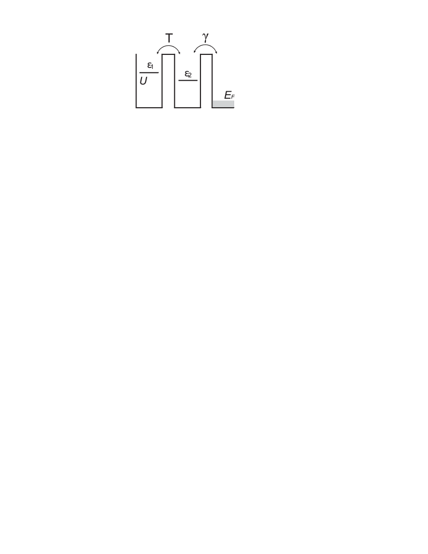
Figure 1: Schematic diagram of energy levels in the system of two coupled QDs. Second QD is also connected with continuous spectrum states.

Different relaxation regimes are determined by the relations between the model parameters: $T$, $\gamma$, $U$ and $\varepsilon_{i}$. QDs electronic states coupling $T$ is determined by the distance between the QDs, the barrier height and localized states energy levels positions. Energy levels positions are strongly connected with the QDs geometry: the width and the depth of potential well associated with each dot. The Coulomb interaction between localized electrons is governed by the localization radius of electronic states within the QDs. The value of tunneling rate $\gamma$ depends on the width and height of the barrier which separates second QD from the lead. So all these parameters can be varied in the real experimental situation. Our model parameters correspond to the experimental situation when one of the vertically stacked interacting QDs is deep and narrow (deep energy levels and Coulomb interaction must be taken into account) and another one is wide and shallow (shallow energy levels and Coulomb interaction is small and can be neglected)Kikoin .

As we are interested in the specific features of the non-stationary time evolution of the initially localized charge within the coupled QDs, we’ll consider the situation when condition $(\varepsilon_{i}-\varepsilon_{F})/\gamma)>>1$ is fulfilled. It means that initial energy levels are situated well above the Fermi level and stationary occupation numbers in the second QD in the absence of coupling between the QDs is of order $\gamma/(\varepsilon_{2}-\varepsilon_{F})<<1$. So the Kondo effect can’t appear in the proposed model and we can also omit the terms corresponding to the stationary solution.

First of all we shall find localized charge relaxation laws in the coupled QDs without Coulomb interaction between localized electrons in the first QD. Let us assume that at the initial moment all charge density in the system is localized in the first QD and has the value $n_{1}(0)$. In the absence of tunneling between the QDs Green functions $G_{11}^{R}(t-t^{{}^{\prime}})$ and $G_{22}^{R}(t-t^{{}^{\prime}})$ can be found from expressions:

$$G_{11}^{R}(t-t^{{}^{\prime}}) = -i\Theta(t-t^{{}^{\prime}})e^{-i\varepsilon_{1}(t-t^{{}^{\prime}})}$$

$$G_{22}^{R}(t-t^{{}^{\prime}}) = -i\Theta(t-t^{{}^{\prime}})e^{-i\varepsilon_{2}(t-t^{{}^{\prime}})-\gamma(t-t^{{}^{\prime}})}$$ (3)

where $\gamma=\pi\nu_{k}^{0}T_{k}^{2}$ is tunneling relaxation rate from the second QD to the continuous spectrum states.

Retarded electron Green’s function $G_{11}^{R}$ determine spectrum re-normalization due to tunneling processes between QDs and can be found exactly from the integral equation:

$$G_{11}^{R}=G_{11}^{0R}+G_{11}^{0R}T^{2}G_{22}^{R}G_{11}^{R}$$ (4)

Acting by inverse operators $G_{11}^{0R-1}$ and $G_{22}^{R-1}$ integral equation (4) can be also presented in the equivalent differential form (except the point $t=t^{{}^{\prime}}$):

$$((i\frac{\partial}{\partial t}-\varepsilon_{2}+i\gamma)(i\frac{\partial}{\partial t}-\varepsilon_{1})-T^{2})G_{11}^{R}(t,t^{{}^{\prime}})=0$$ (5)

Finally, retarded Green function $G_{11}^{R}$ can be written in the following form:

$$G_{11}^{R}(t,t^{{}^{\prime}})=i\Theta(t-t^{{}^{\prime}})(\frac{E_{1}-\varepsilon_{2}+i\gamma}{E_{1}-E_{2}}e^{-E_{1}(t-t^{{}^{\prime}})}-$$

$$-\frac{E_{2}-\varepsilon_{2}+i\gamma}{E_{1}-E_{2}}e^{-E_{2}(t-t^{{}^{\prime}})})$$ (6)

where eigenfrequencies $E_{1,2}$ are determined by the equations:

$$(E-\varepsilon_{1})(E-\varepsilon_{2}+i\gamma)-T^{2}=0$$

$$E_{1,2}=\frac{1}{2}(\varepsilon_{1}+\varepsilon_{2}-i\gamma)\pm\frac{1}{2}\sqrt{(\varepsilon_{1}-\varepsilon_{2}+i\gamma)^{2}+4T^{2}}$$ (7)

Let us now analyze time evolution of the electron density in the considered system which is governed by the Keldysh Green function $G_{11}^{<}(t,t^{{}^{\prime}})$ Keldysh :

$$G_{11}^{<}(t,t^{{}^{\prime}})=in_{1}(t)$$ (8)

Equation for Green function $G_{11}^{<}$ has the form:

$$G_{11}^{<}(t,t^{{}^{\prime}})=G_{11}^{0<}+G_{11}^{0<}T^{2}G_{22}^{A}G_{11}^{A}+$$

$$+G_{11}^{0R}T^{2}G_{22}^{R}G_{11}^{<}+G_{11}^{0R}T^{2}G_{22}^{<}G_{11}^{A}$$

and after acting by $G_{11}^{0R-1}$ can be re-written as:

$$(G_{11}^{0R-1}-T^{2}G_{22}^{R})G_{11}^{<}=T^{2}G_{22}^{<}G_{11}^{A}$$ (10)

Green function $G_{11}^{<}(t,t)$ is determined by the sum of homogeneous and inhomogeneous solutions. Inhomogeneous solution of the equation can be written in the following way:

$$G_{11}^{<}(t,t^{{}^{\prime}})=T^{2}\int_{0}^{t}dt_{1}\int_{0}^{t^{{}^{\prime}}}dt_{2}G_{11}^{R}(t-t_{1})\cdot$$

$$\cdot G_{22}^{<}(t_{1}-t_{2})G_{11}^{A}(t_{2}-t^{{}^{\prime}})$$

If $G_{22}^{<}(0,0)=0$, Green function $G_{11}^{<}(t,t)$ is defined by the solution of homogeneous equation. Homogeneous solution of the differential equation has the form:

$$G_{11}^{<}(t,t^{{}^{\prime}})=f_{1}(t^{{}^{\prime}})e^{-iE_{1}t}+f_{2}(t^{{}^{\prime}})e^{-iE_{2}t}$$ (12)

It is also necessary to satisfy the symmetry relations for function $G^{<}(t,t^{{}^{\prime}})$:

$$(G_{11}^{<}(t,t^{{}^{\prime}}))^{*}=-G_{11}^{<}(t^{{}^{\prime}},t)$$ (13)

We can determine all the coefficients because the solution has to satisfy homogeneous integro-differential equation:

$$G_{11}^{<}(t^{{}^{\prime}},t)=iAe^{-iE_{1}t+iE_{1}^{*}t^{{}^{\prime}}}+iBe^{-iE_{1}t+iE_{2}^{*}t^{{}^{\prime}}}+$$

$$+iB^{*}e^{-iE_{2}t+iE_{1}^{*}t^{{}^{\prime}}}+iCe^{-iE_{2}t+iE_{2}^{*}t^{{}^{\prime}}}$$ (14)

We also have to fulfill initial condition:

$$G_{11}^{<}(0,0)=in_{1}^{0}$$ (15)

As far as solution has to satisfy homogeneous integro-differential equation, after some calculations one can find the following proportionality between $f_{1}(t^{{}^{\prime}})$ and $f_{2}(t^{{}^{\prime}})$:

$$\frac{f_{1}(t^{{}^{\prime}})}{f_{2}(t^{{}^{\prime}})}=-\frac{\varepsilon_{2}-E_{1}-i\gamma}{\varepsilon_{2}-E_{2}-i\gamma}$$ (16)

Finally time dependence of filling numbers in the first QD $n_{1}(t)$ can be written as:

$$n_{1}(t) = n_{1}^{0}\cdot(Ae^{-i(E_{1}-E_{1}^{*})t}+2Re(Be^{-i(E_{1}-E_{2}^{*})t})+$$ (17)

$$+ Ce^{-i(E_{2}-E_{2}^{*})t})$$

where coefficients $A$, $B$ and $C$ are determined as:

$$A = \frac{|E_{2}-\varepsilon_{1}|^{2}}{|E_{2}-E_{1}|^{2}};C=\frac{|E_{1}-\varepsilon_{1}|^{2}}{|E_{2}-E_{1}|^{2}}$$

$$B = -\frac{(E_{2}-\varepsilon_{1})(E_{1}^{*}-\varepsilon_{1})}{|E_{2}-E_{1}|^{2}}$$ (18)

Time evolution of electron density in the second QD is determined by the Green function $G_{22}^{<}(t,t^{{}^{\prime}})$ with initial condition $G_{22}^{<}(0,0)=0$. Green function $G_{22}^{<}(t,t^{{}^{\prime}})$ can be found from equation similar to the equation (10) with the following indexes changing ($1\leftrightarrow 2$). Due to the initial conditions $n_{2}(0)=0$, $n_{1}(0)=n_{0}=1$, filling numbers evolution in the second QD $n_{2}(t)$ is defined by the inhomogeneous part of the solution. So time dependence of the electron filling numbers in the second QD $n_{2}(t)$ can be written as:

$$n_{2}(t) = (De^{-i(E_{1}-E_{1}^{*})t}+2Re(Ee^{-i(E_{1}-E_{2}^{*})t})+$$ (19)

$$+ Fe^{-i(E_{2}-E_{2}^{*})t})$$

where coefficients $D$, $E$ and $F$ are determined by expressions:

$$D=F=-E=\frac{T^{2}}{|E_{2}-E_{1}|^{2}}$$ (20)

It is clearly evident that three typical time scales exist in the considered system in the absence of Coulomb interaction between localized electrons, which are described by the expressions (17),(LABEL:filling_numbers_2). Two of them we shall identify as the first $|E_{1}-E_{1}^{*}|$ and second $|E_{2}-E_{2}^{*}|$ mode correspondingly. One more time scale is defined by the expression $|E_{1}-E_{2}^{*}|$ and results in formation of charge density oscillations in both QDs, when the following ratio between $T$ and $\gamma$ is valid: $T/\gamma>1/\sqrt{2}$. Several time rates in localized charge relaxation in a QD coupled with the thermostat were also found and carefully analyzed in Contreras .

It is necessary to mention that the suggested model can be generalized for the situation when both QDs are connected with the leads. All the expressions up to the equation (20) continue being valid if one substitutes $\varepsilon_{1}$ by the expression $\varepsilon_{1}-i\gamma_{1}$ where $\gamma_{1}$ is a tunneling rate from the first QD to the contact lead. In this paper we are interested in the specific features of charge relaxation processes first of all due to the charge redistribution between the coupled QDs. So we consider strongly asymmetric case when $\gamma_{1}<<\gamma$ and $\gamma_{1}<<T$. In such approximation obtained results can be applied to the system of coupled QDs connected with the both leads. The presented assumptions correspond to the well known experimentally vertically aligned geometry of the coupled QDs Vamivakas ,Stinaff ,Elzerman .

Now we shall take into account on-site Coulomb repulsion within the first QD. We shall confine ourself by analyzing only paramagnetic case when $n_{1\sigma}=n_{1-\sigma}=n_{1}$.

Coulomb interaction within the first QD is considered by means of self-consistent mean field approximation Anderson . It means that in the final expressions for the filling numbers time evolution (17),(19) one have to substitute energy level value $\varepsilon_{1}$ by the value $\widetilde{\varepsilon}_{1}$, which is determined as:

$$\widetilde{\varepsilon}_{1}=\varepsilon_{1}+U+U\cdot(<n_{1}(t)>-1)$$ (21)

We consider charge relaxation from initially filled electronic state in the first QD, and it is reasonable to determine initial energy level position in the first QD as $\varepsilon_{1}+U$, where $\varepsilon_{1}$ is the energy of the empty electronic state. So the initial detuning is $\Delta\varepsilon=\varepsilon_{1}+U-\varepsilon_{2}$ because at $t=0$: $\widetilde{\varepsilon}_{1}=\varepsilon_{1}+U$.

Consequently one should solve self-consistent system of equations (7), (17), (18) and (21) to obtain the new energy level position $\widetilde{\varepsilon}_{1}$ and $n_{1}(t)$. First of all it is necessary to substitute expressions for $E_{1}$ and $E_{2}$ from eq.(7) to the eq.(18) and to determine coefficients $A$, $B$ and $C$. Than one have to substitute $A$, $B$ and $C$ from eq.(18) to the eq.(17). Finally two equations are obtained where equation for $n_{1}(t)$ depends on the new energy level position and equation for $\widetilde{\varepsilon}_{1}$ depends on the filling numbers time evolution $n_{1}(t)$. These two equations can be solved self-consistently. The result of self-consistent solution gives us $n_{1}(t)$ and new energy level position as a functions of time. After this procedure coefficients $D$, $E$, and $F$ can be found from eq. (20). And finally substituting eq.(20) to eq.(19) one can obtain $n_{2}(t)$.

III Calculation results

We shall start our discussion from the resonant case when energy levels in the both QDs are close to each other $\varepsilon_{1}+U\simeq\varepsilon_{2}$. Fig.2a,b demonstrates filling numbers (localized charge) time evolution in the first and second QDs ($n_{1}(t)$ and $n_{2}(t)$) for the different values of Coulomb interaction. It is evident that Coulomb interaction results in the increasing of the relaxation rate (grey line on Fig.2a,b) in comparison with the situation when Coulomb interaction is absent (black line on Fig.2a,b). A particular value of Coulomb interaction exists in the system ($U/\gamma=4$ for a given set of parameters). When Coulomb interaction is lower than $U/\gamma=4$, localized charge relaxation occurs monotonically (Fig.2a,b grey line). Otherwise one can clearly see that relaxation process becomes non-monotonic and reveals several typical time intervals with different values of relaxation rates (black dashed line on Fig.2a,b). Obtained results strongly correspond to the localized charge relaxation peculiarities in the system of coupled QDs when Coulomb interaction is taken into account only within the second QD Mantsevich .

Figure 2: Filling numbers evolution in the first a),c). $n_{1}(t)$ and second b),d). $n_{2}(t)$ QDs. Panels a). and b). correspond to the resonant tunneling $(\varepsilon_{1}-\varepsilon_{2})/\gamma=0.0$. $U=0$-black line, $U=2$-grey line, $U=4$-dashed line. Panels c). and d). correspond to the tunneling between QDs in the presence of detuning $(\varepsilon_{1}=\varepsilon_{2})/\gamma=1.0$. $U=0$-black line, $U=2$-grey line. Parameters $T/\gamma=0.6$ and $\gamma=1.0$ are the same for all the figures.

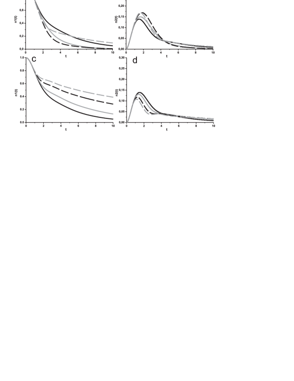
Figure 3: Filling numbers evolution in the first a),c). $n_{1}(t)$ and second b),d). $n_{2}(t)$ QDs. Panels a). and b). correspond to the positive detuning $(\varepsilon_{1}-\varepsilon_{2})/\gamma=1.0$. Panels c). and d). correspond to the negative detuning $(\varepsilon_{1}-\varepsilon_{2})/\gamma=-1.0$. Parameters $T/\gamma=0.6$ and $\gamma=1.0$ are the same for all the figures. $U=0$-black line, $U=0.5$-grey line, $U=1.5$-black dashed line, $U=2.5$-grey dashed line.

Now let us analyze non-resonant case when difference between the energy levels is about the values of parameters $T$ and $\gamma$. We’ll consider different signs of the initial detuning between energy levels. If the detuning has positive value ($\varepsilon_{1}+U>\varepsilon_{2}$) for the small values of Coulomb interaction ($U/\gamma=0.5$, $U/\gamma=1.0$) filling numbers relaxation rate in the first QD increases in comparison with the case when Coulomb interaction is absent (Fig.3a). With the increasing of Coulomb interaction value for $\varepsilon_{2}>\varepsilon_{1}$ the condition $|U(n_{1}(t)-1)|=\Delta\varepsilon$ is fulfilled. So, energy levels detuning turns to zero at the particular time moment. Consequently, resonant tunneling takes place and charge relaxation rate reaches it’s maximum value ($U/\gamma=1.5$ on the Fig.3a). With the further increasing of the Coulomb interaction detuning quickly turns to zero and changes the sign. It results in the decreasing of relaxation rate ($U/\gamma=2.5$ on the Fig.3a). In the opposite case of negative initial energy levels detuning ($\varepsilon_{1}+U<\varepsilon_{2}$) Coulomb interaction results in the increasing of the detuning value and decreasing of the filling numbers relaxation rate in the first QD (Fig.3c). Localized charge relaxation in this case reveals two time intervals with different typical relaxation rate’s scales. Relaxation rate in the first time interval exceeds relaxation rate in the second one.

In the case of strong Coulomb interaction ($U/\gamma=4$ on the Fig.2c,d) one can distinguish three time intervals with different typical relaxation rate’s scales in the electron filling number time evolution. These coincides with the results obtained for the system of coupled QDs when Coulomb interaction between electrons is taken into account within the second QD Mantsevich .

Let us now focus on the most significant result obtained for the system under investigation. It is clearly evident that when energy levels detuning strongly exceeds Coulomb interaction, localized charge relaxation occurs monotonically with a single typical value of relaxation rate (black dashed line on Fig.4a). We revealed that when the Coulomb interaction value within the first QD exceeds the values of tunneling transfer rates ($T$ and $\gamma$) and becomes equal to the value of strong positive detuning between energy levels ($\Delta\varepsilon>>T,\gamma$) in the QDs ($\Delta\varepsilon/\gamma\simeq U/\gamma$) or exceeds it, charge relaxation occurs through two stable regimes which are characterized by significantly different relaxation rate’s values (black and grey lines on Fig.4).

When above-stated conditions are valid at a certain instant of time charge relaxation rate changes discontinuously between two stable values. This phenomenon in the localized charge evolution can be called bifurcation.

With the increasing of Coulomb interaction bifurcation takes place for the smaller time values (black and grey lines on Fig.4a). So one can tune the bifurcation moment by changing the detuning value and the strength of Coulomb interaction.

We have not revealed bifurcations in the case when Coulomb interaction was taken into account within the second QD Mantsevich . The following physical reason as an explanation of this fact can be considered: Localized charge relaxation in the first QD occurs only due to the tunneling processes to the second QD. Relaxation from the second dot is possible due to the coupling between the QDs and also to the transitions to continuous spectrum states. So when Coulomb interaction is taken into account within the first QD the charge relaxation demonstrates much more rough behaviour due to the only one relaxation channel from this QD. It results in the bifurcations formation.

For the detailed analysis of charge relaxation processes we shall carefully examine power law exponents evolution, which determine charge relaxation rates changing in each mode of the QDs (Fig.4c). Moreover we shall analyze time evolution of preexponenial factors which reveal charge distribution among the modes (Fig.4d).

Power law exponents evolution is the same for the both QDs (Fig.4c). When the parameters values correspond to the bifurcation regime in the charge evolution, relaxation rates of the first and second modes demonstrate fast transitions between the two stable values. First mode relaxation rate decreases and second mode relaxation rate increases. After bifurcation both modes reveal identical relaxation rates values (Fig.4c).

Let us now analyze preexponential factors time evolution (mode’s amplitudes) in the presence of Coulomb interaction. In the second QD time evolution of preexponential factors is determined by the same law (expression 20) (Fig.4d). Time evolution of the preexponential factors in the first QD significantly differs (expression 18). When the Coulomb interaction value becomes equal to the detuning value, modes amplitudes demonstrate fast switching between the two stable values. First mode amplitude in the first QD rapidly decreases. Second mode amplitude in the first QD and both mode’s amplitudes in the second QD increase. After bifurcation all mode’s amplitudes admit equal values. It means that Coulomb interaction leads to equal charge re-distribution among the modes in the system of coupled QDs.

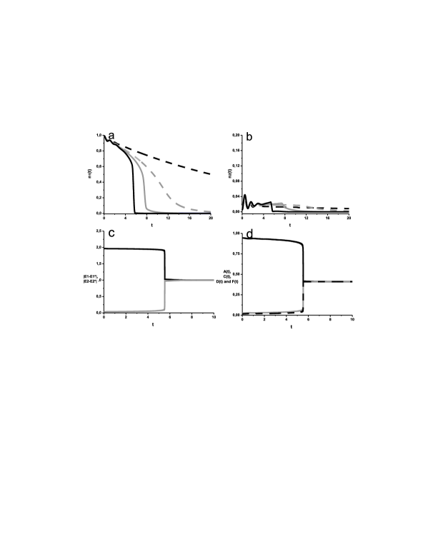
Figure 4: a). Filling numbers evolution in the first QD $n_{1}(t)$. $U=0$-dashed black line, $U=4$-dashed grey line, $U=6$-grey line, $U=7$-black line.; b). Filling numbers evolution in the second QD $n_{2}(t)$. $U=0$-dashed black line, $U=4$-dashed grey line, $U=6$-grey line, $U=7$-black line; c). $|E1-E1^{*}|$-first and $|E2-E2^{*}|$-second mode relaxation rates evolution for $U=7$; d). First mode amplitude in the first QD time evolution $A(t)$-black line; second mode amplitude in the first QD time evolution $C(t)$-grey line; first and second modes in the second QD time evolution $D(t)$ and $F(t)$-dashed black line for $U=7$. Parameters $T/\gamma=0.8$, $\gamma=1.0$ and $(\varepsilon_{1}-\varepsilon_{2})/\gamma=6.0$ are the same for all the figures.

IV Conclusion

We have analyzed time evolution of localized charge in the system of coupled QDs in the presence of Coulomb interaction between electrons within a QD. We have found that Coulomb interaction strongly modifies the relaxation rates and the character of localized charge time evolution. It was shown that several time ranges with considerably different relaxation rates arise in the system of the two coupled QDs. We revealed that at a certain instant of time the system switches rapidly between stable relaxation regimes in a wide range of system parameters. This time moment can be tuned by changing the detuning and Coulomb interaction values. We consider this phenomenon to be applicable for active nano-electronics elements creation based on the effect of fast switching between the two stable states.

This work was partly supported by RFBR and Leading Scientific School grants.

References

- (1) C.P. Collier, E.W. Wong, M. Belohradsky et. al., Science, 285, (1999), 391.
- (2) D.I. Gittins et.al., Nature, 408, (2000), 677.
- (3) M.A. Kastner, Rev. Mod. Phys., 4, (1992), 849.
- (4) R. Ashoori, Nature, 379, (1996), 413.
- (5) T.H. Oosterkamp, T. Fujisawa, W.G. van der Wiel et.al., Nature, 395, (1998), 873.
- (6) R.H. Blick, D. van der Weide, R.J. Haug et.al., Phys.Rev Lett., 81, (1998), 689.
- (7) D. Bimberg, M. Grundmann, N. Ledentsov, Quantum Dot Heterostructures Wiley, New-York, (1999).
- (8) C. Livermore, C.H. Crouch, R.M. Westervelt et.al., Science, 274, (1996), 1332.
- (9) I. Rotter, A.F. Sadreev, Phys. Rev. E, 71, (2005), 036227.
- (10) V.J. Goldman, D.C. Tsui, J.E. Cunningham, Phys. Rev. Lett., 58, (1987), 1256.
- (11) A.N. Vamivakas, C.-Y. Lu, C. matthiesen et.al., Nature Letters, 467, (2010), 297.
- (12) E.A. Stinaff, M. Scheibner, A.S. Bracker et.al., Science, 311, (2006), 636.
- (13) J.M. Elzerman, K.M. Weiss, J. Miguel-Sanchez et.al., Phys. Rev. Lett., 107, (2011), 017401.
- (14) J. Peng, G. Bester, Phys. Rev. B, 82, (2010), 235314.
- (15) G. Munoz-Matutano, M. Royo, J.I. Climente et.al., Phys. Rev. B, 84, (2011), 041308(R).
- (16) S. J. Angus, A.J. Ferguson, A.S. Dzurak et. al., Nano Lett., 7, (2007), 2051.
- (17) K. Grove-Rasmussen, H. Jorgensen, T. Hayashi et. al., Nano Lett., 8, (2008), 1055.
- (18) S. Moriyama, D. Tsuya, E. Watanabe et. al., Nano Lett., 9, (2009), 2891.
- (19) R. Landauer, Science, 272, (1996), 1914.
- (20) P.I. Arseyev, N.S. Maslova, V.N. Mantsevich, arXiv: 1111.5776.
- (21) A.S. Alexandrov, A.M. Bratkovsky, R.S. Williams, Phys.Rev.B, 67, (2003), 075301.
- (22) P.A. Orellana, G.A. Lara, E.V. Anda, Phys.Rev.B, 65, (2002), 155317.
- (23) A.Rack, R. Wetzler, A. Wacker, E. Scholl, Phys.Rev.B, 66, (2002), 165429.
- (24) I.Djuric, C.P. Search, Phys.Rev.B, 75, (2007), 155307.
- (25) P.Coleman, Phys.Rev.B, 29, (1984), 3035.
- (26) P.Coleman, Phys.Rev.B, 35, (1987), 5072.
- (27) R. Wetzler, C.M.A. Kapteyn, R. Heitz, A. Wacker, E. Sholl, D. Bimberg, Appl.Phys. Lett., 77, (2000), 1671.
- (28) J.Hubbard, Proc.Roy.Soc.A, 276, (1963), 238.
- (29) A.S. Alexandrov, A.M. Bratkovsky, R.S. Williams, Phys.Rev.B, 67, (2003), 075301.
- (30) L.V. Keldysh, Sov. Phys. JETP, 20, (1964), 1018.
- (31) K.Kikoin, Y. Avishai, Phys.Rev.Lett., 86, (2001), 2090.
- (32) L.D. Contreras-Pulido, J. Splettstoesser, M. Governale, et.al., arXiv: 1111.4135
- (33) P.W. Anderson, Phys.Rev., 124, (1961), 41.