Efficient quantification of non-Gaussian spin distributions

Abstract

We study theoretically and experimentally the quantification of non-Gaussian distributions via non-destructive measurements. Using the theory of cumulants, their unbiased estimators, and the uncertainties of these estimators, we describe a quantification which is simultaneously efficient, unbiased by measurement noise, and suitable for hypothesis tests, e.g., to detect non-classical states. The theory is applied to cold ⁸⁷Rb spin ensembles prepared in non-gaussian states by optical pumping and measured by non-destructive Faraday rotation probing. We find an optimal use of measurement resources under realistic conditions, e.g., in atomic ensemble quantum memories.

Introduction - Non-Gaussian states are an essential requirement for universal quantum computation Ralph et al. (2003); Lloyd and Braunstein (1999) and several quantum communication tasks with continuous variables, including improving the fidelity of quantum teleportation Dell’Anno et al. (2007) and entanglement distillation Eisert et al. (2002); Giedke and Ignacio Cirac (2002). Optical non-Gaussian states have been demonstrated Neergaard-Nielsen et al. (2006); Ourjoumtsev et al. (2007); Wakui et al. (2007); Takahashi et al. (2008); Ježek et al. (2011) and proposals in atomic systems Massar and Polzik (2003); Nielsen et al. (2009); Lemr and Fiurášek (2009); Mazets et al. (2008) are being actively pursued. In photonic systems, histograms Wenger et al. (2004) and state tomography Ježek et al. (2011); Neergaard-Nielsen et al. (2006); Ourjoumtsev et al. (2007); Takahashi et al. (2008) have been used to show non-Gaussianity, but require a large number of measurements. For material systems with longer time-scales these approaches may be prohibitively expensive. Here we demonstrate the use of cumulants, global measures of distribution shape, to show non-Gaussianity in an atomic spin ensemble. Cumulants can be used to show non-classicality Bednorz and Belzig (2011); Shchukin et al. (2005); Eran Kot and Sørensen (2011), can be estimated with few measurements and have known uncertainties, a critical requirement for proofs of non-classicality.

Approach - Quantification or testing of distributions has features not encountered in quantification of observables. For example, experimental measurement noise appears as a distortion of the distribution that cannot be “averaged away” by additional measurements. As will be discussed later, the theory of cumulants naturally handles this situation. We focus on the fourth-order cumulant $\kappa_{4}$, the lowest-order indicator of non-Gaussianity in symmetric distributions such as Fock Lvovsky et al. (2001) and “Schrödinger kitten” states Ourjoumtsev et al. (2007); Massar and Polzik (2003). We study theoretically and experimentally the noise properties of Fisher’s unbiased estimator of $\kappa_{4}$, i.e., the fourth “k-statistic” $k_{4}$, and find optimal measurement conditions. Because $\kappa_{4}$ is related to the negativity of the Wigner function Bednorz and Belzig (2011), this estimation is of direct relevance to detection of non-classical states. We employ quantum non-demolition measurement, a key technique for generation and measurement of non-classical states in atomic spin ensembles Appel et al. (2009); Koschorreck et al. (2010a) and nano-mechanical oscillators Hertzberg et al. (2010).

Moments, cumulants and estimators - A continuous random variable $X$ with probability distribution function $P(X)$ is completely characterized by its moments ${{\mu}}_{k}\equiv\int X^{k}P(X)dX$ or cumulants ${\kappa}_{n}=\mu_{n}-\sum_{k=1}^{n-1}\left({}^{n-1}_{k-1}\right)\mu_{n-k}{\kappa}_{k}$, where $\left({}^{n}_{k}\right)$ is the binomial coefficient.

Since Gaussian distributions have $\kappa_{n>2}=0$, estimation of $\kappa_{4}$, (or $\kappa_{3}$ for non-symmetric distributions), is a natural test for non-Gaussianity. In an experiment, a finite sample $\{X_{1}\ldots X_{N}\}$ from $P$ is used to estimate the $\kappa$’s. Fisher’s unbiased estimators, known as “k-statistics” $k_{n}$, give the correct expectation values $\left<k_{n}\right>=\kappa_{n}$ for finite $N$ Kendall and Stuart (1958). Defining $S_{n}=\sum_{i}X_{i}^{n}$ we have:

$${k}_{3} = ({2S_{1}^{3}-3NS_{1}S_{2}+N^{2}S_{3}})/N_{(2)}$$ (1)

$${k}_{4} = \left(-6S_{1}^{4}+12NS_{1}^{2}S_{2}-3N(N-1)S_{2}^{2}\right.$$ (2)

$$\left.-4N(N-1)S_{1}S_{3}+N^{2}(N+1)S_{4}\right)/N_{(3)}$$

where $N_{(m)}\equiv N(N-1)\ldots(N-m)$ .

We need the uncertainty in the cumulant estimation to test for non-Gaussianity, or to compare non-Gaussianity between distributions. For hypothesis testing and maximum-likelihood approaches, we need the variances of $k_{3},k_{4}$ for a given $P$. These are found by combinatorial methods and given in reference Kendall and Stuart (1958):

$${\rm var}(k_{3}) = {{\kappa}_{6}}/{N}+9N({\kappa}_{2}{\kappa}_{4}+{\kappa}_{3}^{2})/N_{(1)}+6N^{2}{\kappa}_{2}^{3}/N_{(2)}\;\;\;\;\;$$ (3)

$${\rm var}(k_{4}) = {{\kappa}_{8}}/{N}+2N({8{\kappa}_{6}{\kappa}_{2}+24{\kappa}_{5}{\kappa}_{3}+17{\kappa}_{4}^{2}})/N_{(1)}$$ (4)

$$+72N^{2}({{\kappa}_{4}{\kappa}_{2}^{2}+2{\kappa}_{3}^{2}{\kappa}_{2}})/N_{(2)}$$

$$+{24N^{2}(N+1){\kappa}_{2}^{4}}/N_{(3)}.$$

It is also possible to estimate the uncertainty in $k_{4}$ from data $\{X\}$ using estimators of higher order cumulants Kendall and Stuart (1958). The efficiency of cumulant estimation is illustrated in Fig. 1.

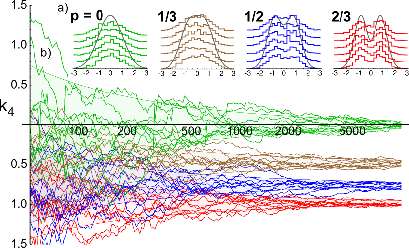
Figure 1: (color online) Simulated estimator $k_{4}$ as a function of sample size $N$. a) (insets) black curves show quadrature distributions of states $\rho=(1-p)\left|0\right>\left<0\right|+p\left|1\right>\left<1\right|$, scaled to unit variance, and six $N=1000$ histograms (offset for clarity) for $p=0$ (green), $1/3$ (brown), $1/2$ (blue) and $2/3$ (red). b) Ten realizations of $k_{4}$ versus $N$ drawn from each of the four distributions. Shaded regions show $\kappa_{4}\pm\sqrt{{\rm var}(k_{4})}$, from Eqs (2), (4). With $N=1000$, $k_{4}$ distinguishes $p=1/2$ (blue) from $p=0$ (green, Gaussian) with $>7\sigma$ significance, even though the histograms look similar “to the eye.”

Measurement noise - When the measured signal is $Z=X+Y$, where $X$ is the true value and $Y$ is uncorrelated noise, the measured distribution is the convolution $P(Z)=P(X)\otimes P(Y)$. The effect of this distortion on cumulants is the following: for independent variables, cumulants accumulate (i.e., add) Kendall and Stuart (1958), so that $\kappa_{n}^{(Z)}=\kappa_{n}^{(X)}+\kappa_{n}^{(Y)}$, where $\kappa_{n}^{(Q)},k_{n}^{(Q)}$ indicate $\kappa_{n},k_{n}$ for distribution $P(Q)$. The extremely important case of uncorrelated, zero-mean Gaussian noise, $\kappa_{2}^{(Y)}=\sigma^{2}_{Y}$ and other cumulants zero, is thus very simple: $\kappa_{n}^{(Z)}=\kappa_{n}^{(X)}$ except for $\kappa_{2}^{(Z)}=\kappa_{2}^{(X)}+\sigma^{2}_{Y}$. Critically, added Gaussian noise does not alter the observed $\kappa_{3}$, $\kappa_{4}$.

Experimental system and state preparation - We test this approach by estimating non-Gaussian spin distributions in an atomic ensemble, similar to ensemble systems being developed for quantum networking with non-Gaussian states Polzik and Müller . The collective spin component $F_{z}$ is measured by Faraday rotation using optical pulses. The detected Stokes operator is $S_{y}^{(\rm out)}=S_{y}^{(\rm in)}+GN_{\rm L}F_{z}/2$, where $G$ is a coupling constant, $N_{\rm L}$ is the number of photons, and $S_{y}^{(\rm in)}$ is the input Stokes operator, which contributes quantum noise. In the above formulation $X=F_{z},$ $Y=2S_{y}^{(\rm in)}/(GN_{\rm L})$ and $Z=2S_{y}^{(\rm out)}/(GN_{\rm L})$.

The experimental system is described in detail in references Kubasik et al. (2009); Koschorreck et al. (2010b, a). An ensemble of $\sim 10^{6}~{}^{87}$Rb atoms is trapped in an elongated dipole trap made from a weakly focused $1030\text{\,}\mathrm{n}\mathrm{m}$ beam and cooled to $25\text{\,}\mathrm{\SIUnitSymbolMicro}\mathrm{K}$. A non-destructive measurement of the atomic state is made using pulses of linearly polarized light detuned $800\text{\,}\mathrm{M}\mathrm{H}\mathrm{z}$ to the red of the $F=1\,\rightarrow\,F^{\prime}=0$ transition of the D₂ line and sent through the atoms in a beam matched to the transverse cloud size. The pulses are of $1\text{\,}\mathrm{\SIUnitSymbolMicro}\mathrm{s}$ duration, contain $3.7\times 10^{6}$ photons on average, and are spaced by $10\text{\,}\mathrm{\SIUnitSymbolMicro}\mathrm{s}$ to allow individual detection. The 240:1 aspect ratio of the atomic cloud creates a strong paramagnetic Faraday interaction

$G\approx{6\times 10^{-8}}$ rad/spin. After interaction with the atoms, $S_{y}^{(\rm out)}$ is detected with a shot noise limited (SNL) balanced polarimeter in the $\pm 45^{\circ}$ basis. $N_{\rm L}$ is measured with a beam-splitter and reference detector before the atoms. The probing-plus-detection system is shot-noise-limited above $3\times 10^{5}$ photons/pulse. Previous work with this system has demonstrated QND measurement of the collective spin $F_{z}$ with an uncertainty of $\sim 500$ spins Koschorreck et al. (2010b, a).

We generate Gaussian and non-Gaussian distributions with the following strategy: we prepare a “thermal state” (TS), an equal mixture of the $F=1,m_{F}=-1,0,1$ ground states, by repeated unpolarized optical pumping between the $F=1$ and $F=2$ hyperfine levels, finishing in $F=1$ Koschorreck et al. (2010b). By the central limit theorem, the TS of $10^{6}$ atoms is nearly Gaussian with $\left<F_{z}\right>=0$ and ${\rm var}(F_{z})=\sigma^{2}=2N_{A}/3$. By optical pumping with pulses of circularly-polarized light we displace this to $\left<F_{z}\right>=\alpha$, with negligible change in ${\rm var}(F_{z})$ Tóth and Mitchell (2010), to produce $P_{\alpha}(F_{z})=(\sigma\sqrt{2\pi})^{-1}\exp[-(F_{z}-\alpha)^{2}/(2\sigma^{2})]$. By displacing different TS alternately to $\alpha_{+}$ and $\alpha_{-}$, we produce an equal statistical mixture of the two displaced states, $P_{\alpha}^{\rm(NG)}(F_{z})=[P_{\alpha_{+}}(F_{z})+P_{\alpha_{-}}(F_{z})]/2$. With properly-chosen $\alpha_{\pm}$, $P_{\alpha}^{\rm(NG)}(F_{z})$ closely approximates marginal distributions of mixtures of $n=0,1$ Fock states and $m=N,N-1$ symmetric Dicke states. The experimental sequence is shown in Fig. 2.

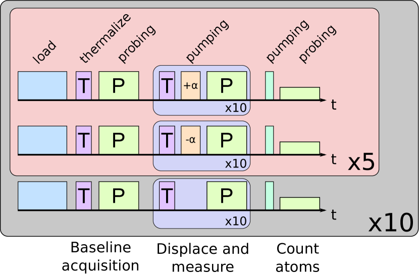
Figure 2: Experimental sequence: The experimental sequence divides into distinct tasks. Baseline acquisition: prepare the thermal state and probe to measure the residual rotation. Displace and measure (DM[$\alpha$]): prepare the thermal state, displace by $\alpha$ and probe. Thanks to atom loss at each thermalization, the atom number is varied by repeating DM several times. Measure number of atoms $N_{A}$: by pumping the atoms into F=1, $m_{F}$=1 and probing we measure the number of atoms in the trap. To correct for drifts, a sequence without displacement (DM[0]) is performed every 11 runs. We perform the sequence varying the displacement to acquire a dataset of quantum-noise-limited measurements of $P_{\alpha}^{(\rm NG)}(S_{y}^{(\rm out)})$ for different $\alpha$.

Detection, Analysis and Results - For each preparation, 100 measurements of $F_{z}$ are made, with readings (i.e., estimated $F_{z}$ values by numerical integration of the measured signal) $m_{i}=2S_{y}^{({\rm out},i)}/N_{L}^{(i)}$. Because the measurement is non-destructive and shot noise limited, we can combine $N_{R}$ readings in a higher-sensitivity metapulse with reading $M\equiv\sum m_{i}$ Koschorreck et al. (2010b). This has the distribution $P_{\alpha_{\pm}}(M)=\exp[-(M-\alpha_{\pm})^{2}/(2\sigma_{M}^{2})]/(\sigma_{M}\sqrt{2\pi})$ where the variance $\sigma_{M}^{2}=\sigma_{A}^{2}{N_{A}^{\prime}}^{2}N_{R}^{2}+\sigma_{R}^{2}$ includes atomic noise $\sigma_{A}^{2}{N_{A}^{\prime}}^{2}$ and readout noise, $\sigma_{R}^{2}=N_{R}/N_{L}$ with $N_{A}^{\prime}=N_{A}/N_{A}^{MAX}$ . The variance $\sigma_{A}^{2}$ is determined from the scaling of ${\rm var}(M)$ with $N_{A}$ and $N_{R}$, as in Koschorreck et al. (2010b). The readout noise can be varied over two orders of magnitude by appropriate choice of $N_{R}$. For one probe pulse and the maximum number of atoms we have $\sigma_{R}^{2}/\sigma_{A}^{2}=84.7$.

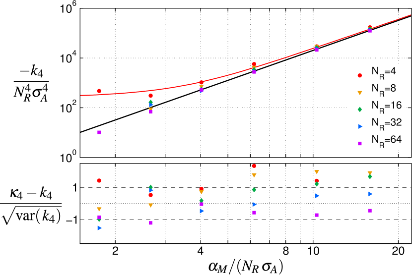
Figure 3: (color online) Measured and predicted $k_{4}$ with residuals for non-Gaussian distributions of different $\alpha$. Readout noise is varied by the choice of $N_{R}$. Data is normalized to $N_{R}$ and $\sigma_{A}$. Top: Points show normalized $-k_{4}$ calculated from $N=100$ preparations of the ensemble with different $\alpha$ (horizontal axis), and $N_{R}$ (colors). Black line indicates expected $-\kappa_{4}$, red line (top) shows $-\kappa_{4}+\sqrt{{\rm var}(k_{4})}$ calculated from the distribution parameters for the largest readout noise. Bottom: normalized residuals $(-k4+\kappa_{4})/\sqrt{{\rm var}(k_{4})}$. The normalization is done with the expected ${\rm var}(k_{4})$ for each $N_{R}$. Measured $k_{4}$ agrees well with theory, in particular, measurement noise increases the observed variance, but not the expectation.

To produce a non-Gaussian distribution, we compose metapulses from $N_{R}$ samples drawn from displaced thermal state (DM[$\alpha_{+}$] or DM[$\alpha_{-}$]) preparations with equal probability, giving distribution $P_{\alpha}^{(\rm NG)}(M)=[P_{\alpha_{+}}(M)+P_{\alpha_{-}}(M)]/2$. With $\alpha_{M}\equiv(\alpha_{+}-\alpha_{-})/2$, the distribution has $\kappa_{2n+1}=0$, $\kappa_{2}=\alpha_{M}^{2}+\sigma_{M}^{2}$, $\kappa_{4}=-2\alpha_{M}^{4}$, $\kappa_{6}=16\alpha_{M}^{6}$, $\kappa_{8}=-272\alpha_{M}^{8}$. Our ability to measure the non-Gaussianity is determined by $\left<k_{4}\right>=\kappa_{4}$ and from Eq (4)

$${\rm var}(k_{4}) = 136N\alpha_{M}^{8}/N_{(1)}-144N^{2}\alpha_{M}^{4}(\alpha_{M}^{2}+\sigma_{M}^{2})^{2}/N_{(2)}$$ (5)

$$+24N^{2}(N+1)(\alpha_{M}^{2}+\sigma_{M}^{2})^{4}/N_{(3)}.$$

As shown in Fig. 3, the experimentally obtained values agree well with theory, and confirm the independence from measurement noise.

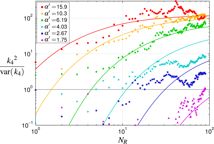
Figure 4: (color online) Signal-to-noise in estimation of $\kappa_{4}$ versus readout noise for different $\alpha^{\prime}=\alpha_{M}/(N_{R}\,\sigma_{A})$. Points show measurement results, lines show theory. (details in the text)

The “signal-to-noise ratio” for $\kappa_{4}$, $S={\kappa_{4}}^{2}/{\rm var}(k_{4})$, is computed using Eq. (5), $\kappa_{4}=-2\alpha^{4}_{M}$, and experimental $\alpha_{M}$, $N_{R}$, $\sigma_{R}$, is shown as curves in Fig 4. We can confirm this $S$ experimentally by computing $S_{N}\equiv\left<k_{4}\right>^{2}/{\rm var}(k_{4})$ using $k_{4}$ values derived from several realizations of the experiment, each sampling $P_{\alpha}^{NG}$ $N$ times. In the limit of many realizations $S_{N}\rightarrow S$. We employ a bootstrapping technique: From 100 samples of $P_{\alpha}^{(\rm NG)}(M)$ for given parameters $\alpha_{M},N_{R}$ and $N_{A}$, we derive thirty-three $N=20$ realizations by random sampling without replacement, and compute $\left<k_{4}\right>$ and ${\rm var}(k_{4})$ on the realizations. As shown in Fig. 4, good agreement with theory is observed.

Optimum estimation of non-Gaussian distributions - Finally, we note that in scenarios where measurements are expensive relative to state preparation (as might be the case for QND measurements of optical fields or for testing the successful storage of a single photon in a quantum memory), optimal use of measurement resources (e.g. measurement time) avoids both too few preparations and too few probings.

We consider a scenario of practical interest for quantum networking: a heralded single-photon state is produced and stored in an atomic ensemble quantum memory. Assuming the ensemble is initially polarized in the $\hat{X}$ direction, the storage process maps the quadrature components $X,P$ onto the corresponding atomic spin operators $X_{A},P_{A}\propto F_{z},-F_{y}$, respectively. QND measurements of $F_{z}$ are used to estimate $X_{A}$, and thus the non-Gaussianity of the stored single photon. Due to imperfect storage, this will have the distribution of a mixture of $n=0$ and $n=1$ Fock states: $\rho=(1-p)\left|0\rangle\langle 0\right|+p\left|1\rangle\langle 1\right|$. For a quadrature $X$, we have the following probability distribution $P_{p}(X)=\exp[{-{x^{2}}/(2\sigma_{0}^{2})}]\left(px^{2}/\sigma_{0}^{2}+1-p\right)/\left(\sqrt{2\pi}\sigma_{0}\right)$, where $\sigma_{0}$ is the width of the $n=0$ state.

Taking in account the readout noise $\sigma_{R}^{2}$, the cumulants are $\kappa_{\rm odd}=0$, $\kappa_{2}=(2p+1)\sigma_{H}^{2}+\sigma_{R}^{2}$, $\kappa_{4}=-12p^{2}\sigma_{H}^{4}$, $\kappa_{6}=240p^{3}\sigma_{H}^{6}$, $\kappa_{8}=-10080p^{4}\sigma_{H}^{8}$, where the readout noise $\sigma_{R}^{2}$ is included as above. Here $\kappa_{4}$ is directly related to the classicality of the state, since $p>0.5$ implies a negative Wigner distribution Lvovsky et al. (2001).

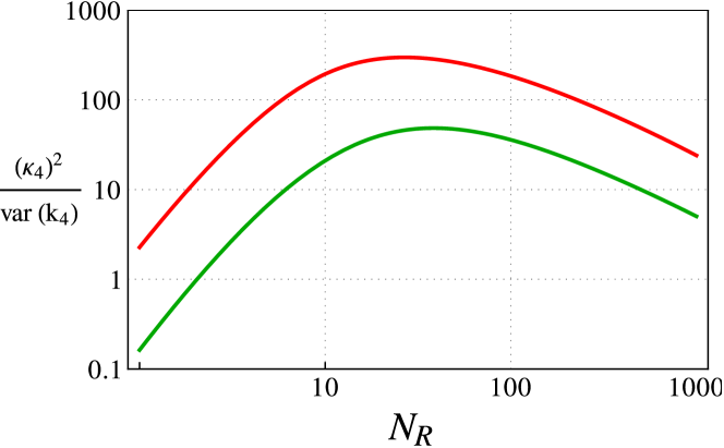
Figure 5: (color online) Signal-to noise-ratio $S$ versus $N_{R}$ for a fixed probe number $N_{M}N_{R}=$1\text{\times}{10}^{5}$$ for the probability distribution associated with Fock state mixture described in the text with a normalized n=0 width $\sigma_{0}=1$. Red curve (top): p=1. Green curve (bottom): p= 0.5 with SNL measurement: $\sigma_{R}=\sqrt{20/N_{R}}$.

For a fixed total number of measurement resources $N_{M}N_{R}$, an optimal distribution of resources per measurement $N_{R}$ exists as shown in Fig. 5. With increasing $N_{R}$, the signal-to-noise first increases due to the improvement of the measurement precision. Then, once the increased measurement precision no longer gives extra information about $k_{4}$, the precision decreases due to reduced statistics because of the limited total number of probes. For a large total number of measurements, we can derive a simplified expression of this optimum. We derive asymptotic expressions of $S$: $S_{L}$ ($S_{H}$) for $\sigma_{R}\ll\sigma_{0}$ ($\sigma_{R}\gg\sigma_{0}$). The optimal $N_{R}$ is found by solving $S_{L}=S_{R}$ giving ${\sigma_{R}}^{8}\approx\sigma_{0}^{8}(1+8p-12p^{2}+48p^{3}-24p^{4})$. For this optimal $\sigma_{R}$, the measurement noise is in the same order of magnitude as the characteristic width of the non-Gaussian distribution.

Conclusion - The cumulant-based methods described here should be very attractive for experiments with non-Gaussian states of material systems such as atomic ensembles and nano-resonators, for which the state preparation time is intrinsically longer, and for which measurement noise is a greater challenge than in optical systems. Cumulant-based estimation is simultaneously efficient, requiring few preparations and measurements, accommodates measurement noise in a natural way, and facilitates statistically-meaningful tests, e.g., of non-classicality. Experimental tests with a cold atomic ensemble demonstrate the method in a system highly suitable for quantum networking, while the theory applies equally to other quantum systems of current interest.