Energy and Spectral Efficiency of Very Large Multiuser MIMO Systems

Abstract

A multiplicity of autonomous terminals simultaneously transmits data streams to a compact array of antennas. The array uses imperfect channel-state information derived from transmitted pilots to extract the individual data streams. The power radiated by the terminals can be made inversely proportional to the square-root of the number of base station antennas with no reduction in performance. In contrast if perfect channel-state information were available the power could be made inversely proportional to the number of antennas. Lower capacity bounds for maximum-ratio combining (MRC), zero-forcing (ZF) and minimum mean-square error (MMSE) detection are derived. A MRC receiver normally performs worse than ZF and MMSE. However as power levels are reduced, the cross-talk introduced by the inferior maximum-ratio receiver eventually falls below the noise level and this simple receiver becomes a viable option. The tradeoff between the energy efficiency (as measured in bits/J) and spectral efficiency (as measured in bits/channel use/terminal) is quantified. It is shown that the use of moderately large antenna arrays can improve the spectral and energy efficiency with orders of magnitude compared to a single-antenna system.

I Introduction

In multiuser multiple-input multiple-output (MU-MIMO) systems, a base station (BS) equipped with multiple antennas serves a number of users. Such systems have attracted much attention for some time now [3]. Conventionally, the communication between the BS and the users is performed by orthogonalizing the channel so that the BS communicates with each user in separate time-frequency resources. This is not optimal from an information-theoretic point of view, and higher rates can be achieved if the BS communicates with several users in the same time-frequency resource [4, 5]. However, complex techniques to mitigate inter-user interference must then be used, such as maximum-likelihood multiuser detection on the uplink [6], or “dirty-paper coding” on the downlink [7, 8].

Recently, there has been a great deal of interest in MU-MIMO with very large antenna arrays at the BS. Very large arrays can substantially reduce intracell interference with simple signal processing [9]. We refer to such systems as “very large MU-MIMO systems” here, and with very large we mean arrays comprising say a hundred, or a few hundreds, of antennas, simultaneously serving tens of users. The design and analysis of very large MU-MIMO systems is a fairly new subject that is attracting substantial interest [10, 9, 11, 12]. The vision is that each individual antenna can have a small physical size, and be built from inexpensive hardware. With a very large antenna array, things that were random before start to look deterministic. As a consequence, the effect of small-scale fading can be averaged out. Furthermore, when the number of BS antennas grows large, the random channel vectors between the users and the BS become pairwisely orthogonal [11]. In the limit of an infinite number of antennas, with simple matched filter processing at the BS, uncorrelated noise and intracell interference disappear completely [9]. Another important advantage of large MIMO systems is that they enable us to reduce the transmitted power. On the uplink, reducing the transmit power of the terminals will drain their batteries slower. On the downlink, much of the electrical power consumed by a BS is spent by power amplifiers and associated circuits and cooling systems [13]. Hence reducing the emitted RF power would help in cutting the electricity consumption of the BS.

This paper analyzes the potential for power savings on the uplink of very large MU-MIMO systems. We derive new capacity bounds of the uplink for finite number of BS antennas. These results are different from recent results in [15] and [16]. In [15] and [16], the authors derived a deterministic equivalent of the SINR assuming that the number of transmit antennas and the number of users go to infinity but their ratio remains bounded for the downlink of network MIMO systems using a sophisticated scheduling scheme and MISO broadcast channels using zero-forcing (ZF) precoding, respectively. While it is well known that MIMO technology can offer improved power efficiency, owing to both array gains and diversity effects [14], we are not aware of any work that analyzes power efficiency of MU-MIMO systems with receiver structures that are realistic for very large MIMO. We consider both single-cell and multicell systems, but focus on the analysis of single-cell MU-MIMO systems since: i) the results are easily comprehensible; ii) it bounds the performance of a multicell system; and iii) the single-cell performance can be actually attained if one uses successively less-aggressive frequency-reuse (e.g., with reuse factor $3$, or $7$). The paper makes the following specific contributions:

• We show that, when the number of BS antennas $M$ grows without bound, we can reduce the transmitted power of each user proportionally to $1/M$ if the BS has perfect channel state information (CSI), and proportionally to $1/\sqrt{M}$ if CSI is estimated from uplink pilots. This holds true even when using simple, linear receivers. We also derive closed-form expressions of lower bounds on the uplink achievable rates for finite $M$, for the cases of perfect and imperfect CSI, assuming MRC, ZF, and minimum mean-squared error (MMSE) receivers, respectively. See Section III.

• We study the tradeoff between spectral efficiency and energy efficiency. For imperfect CSI, in the low transmit power regime, we can simultaneously increase the spectral-efficiency and energy-efficiency. We further show that in large-scale MIMO, very high spectral efficiency can be obtained even with simple MRC processing at the same time as the transmit power can be cut back by orders of magnitude and that this holds true even when taking into account the losses associated with acquiring CSI from uplink pilots. MRC also has the advantage that it can be implemented in a distributed manner, i.e., each antenna performs multiplication of the received signals with the conjugate of the channel, without sending the entire baseband signal to the BS for processing. See Section IV.

II System Model and Preliminaries

II-A MU-MIMO System Model

We consider the uplink of a MU-MIMO system. The system includes one BS equipped with an array of $M$ antennas that receive data from $K$ single-antenna users. The nice thing about single-antenna users is that they are inexpensive, simple, and power-efficient, and each user still gets typically high throughput. Furthermore, the assumption that users have single antennas can be considered as a special case of users having multiple antennas when we treat the extra antennas as if they were additional autonomous users. The users transmit their data in the same time-frequency resource. The $M\times 1$ received vector at the BS is

$${\boldsymbol{y}}=\sqrt{p_{\mathrm{u}}}{\boldsymbol{G}}{\boldsymbol{x}}+{\boldsymbol{n}}$$ (1)

where ${\boldsymbol{G}}$ represents the $M\times K$ channel matrix between the BS and the $K$ users, i.e., $g_{mk}\triangleq\left[{\boldsymbol{G}}\right]_{mk}$ is the channel coefficient between the $m$th antenna of the BS and the $k$th user; $\sqrt{p_{\mathrm{u}}}{\boldsymbol{x}}$ is the $K\times 1$ vector of symbols simultaneously transmitted by the $K$ users (the average transmitted power of each user is $p_{\mathrm{u}}$); and ${\boldsymbol{n}}$ is a vector of additive white, zero-mean Gaussian noise. We take the noise variance to be $1$, to minimize notation, but without loss of generality. With this convention, $p_{\mathrm{u}}$ has the interpretation of normalized “transmit” SNR and is therefore dimensionless. The model (1) also applies to wideband channels handled by OFDM over restricted intervals of frequency.

The channel matrix ${\boldsymbol{G}}$ models independent fast fading, geometric attenuation, and log-normal shadow fading. The coefficient $g_{mk}$ can be written as

$$g_{mk}=h_{mk}\sqrt{\beta_{k}},~{}~{}~{}m=1,2,...,M$$ (2)

where $h_{mk}$ is the fast fading coefficient from the $k$th user to the $m$th antenna of the BS. $\sqrt{\beta_{k}}$ models the geometric attenuation and shadow fading which is assumed to be independent over $m$ and to be constant over many coherence time intervals and known a priori. This assumption is reasonable since the distances between the users and the BS are much larger than the distance between the antennas, and the value of ${\beta_{k}}$ changes very slowly with time. Then, we have

$${\boldsymbol{G}}={\boldsymbol{H}}{\boldsymbol{D}}^{1/2}$$ (3)

where ${\boldsymbol{H}}$ is the $M\times K$ matrix of fast fading coefficients between the $K$ users and the BS, i.e., $\left[{\boldsymbol{H}}\right]_{mk}=h_{mk}$, and ${\boldsymbol{D}}$ is a $K\times K$ diagonal matrix, where $\left[{\boldsymbol{D}}\right]_{kk}=\beta_{k}$. Therefore, (1) can be written as

$${\boldsymbol{y}}=\sqrt{p_{\mathrm{u}}}{\boldsymbol{H}}{\boldsymbol{D}}^{1/2}{\boldsymbol{x}}+{\boldsymbol{n}}.$$ (4)

II-B Review of Some Results on Very Long Random Vectors

We review some limit results for random vectors [18] that will be useful later on. Let ${\boldsymbol{p}}\triangleq\left[p_{1}~{}...~{}p_{n}\right]^{T}$ and ${\boldsymbol{q}}\triangleq\left[q_{1}~{}...~{}q_{n}\right]^{T}$ be mutually independent $n\times 1$ vectors whose elements are i.i.d. zero-mean random variables (RVs) with $\operatorname{\mathbb{E}}\left\{{\left|p_{i}\right|^{2}}\right\}=\sigma_{p}^{2}$, and $\operatorname{\mathbb{E}}\left\{{\left|q_{i}\right|^{2}}\right\}=\sigma_{q}^{2}$, $i=1,...,n$. Then from the law of large numbers,

$$\frac{1}{n}{\boldsymbol{p}}^{H}{\boldsymbol{p}}\mathop{\to}\limits^{a.s.}\sigma_{p}^{2},~{}\text{and}~{}~{}\frac{1}{n}{\boldsymbol{p}}^{H}{\boldsymbol{q}}\mathop{\to}\limits^{a.s.}0,~{}\text{as}~{}n\rightarrow\infty.$$ (5)

where $\mathop{\to}\limits^{a.s.}$ denotes the almost sure convergence. Also, from the Lindeberg-Lévy central limit theorem,

$$\frac{1}{\sqrt{n}}{\boldsymbol{p}}^{H}{\boldsymbol{q}}\mathop{\to}\limits^{d}\mathcal{CN}\left({0},{\sigma_{p}^{2}\sigma_{q}^{2}}\right),~{}\text{as}~{}n\rightarrow\infty$$ (6)

where $\mathop{\to}\limits^{d}$ denotes convergence in distribution.

II-C Favorable Propagation

Throughout the rest of the paper, we assume that the fast fading coefficients, i.e., the elements of ${\boldsymbol{H}}$ are i.i.d. RVs with zero mean and unit variance. Then the conditions in (5)–(6) are satisfied with ${\boldsymbol{p}}$ and ${\boldsymbol{q}}$ being any two distinct columns of ${\boldsymbol{G}}$. In this case we have

$$\frac{{\boldsymbol{G}}^{H}{\boldsymbol{G}}}{M}={\boldsymbol{D}}^{1/2}\frac{{\boldsymbol{H}}^{H}{\boldsymbol{H}}}{M}{\boldsymbol{D}}^{1/2}\approx{\boldsymbol{D}},\quad M\gg K$$

and we say that we have favorable propagation. Clearly, if all fading coefficients are i.i.d. and zero mean, we have favorable propagation. Recent channel measurements campaigns have shown that multiuser MIMO systems with large antenna arrays have characteristics that approximate the favorable-propagation assumption fairly well [11], and therefore provide experimental justification for this assumption.

To understand why favorable propagation is desirable, consider an $M\times K$ uplink (multiple-access) MIMO channel ${\boldsymbol{H}}$, where $M\geq K$, neglecting for now path loss and shadowing factors in ${\boldsymbol{D}}$. This channel can offer a sum-rate of

$$R=\sum_{k=1}^{K}\log_{2}\left(1+{p_{\mathrm{u}}}\lambda_{k}^{2}\right)$$ (7)

where $p_{\mathrm{u}}$ is the power spent per terminal and $\{\lambda_{k}\}_{k=1}^{K}$ are the singular values of ${\boldsymbol{H}}$, see [14]. If the channel matrix is normalized such that $|H_{ij}|\sim 1$ (where $\sim$ means equality of the order of magnitude), then $\sum_{k=1}^{K}\lambda_{k}^{2}=\|{\boldsymbol{H}}\|^{2}\approx MK$. Under this constraint the rate $R$ is bounded as

$$\log_{2}\left(1+MKp_{\mathrm{u}}\right)\leq R\leq K\log_{2}\left(1+{M}p_{\mathrm{u}}\right)$$ (8)

The lower bound (left inequality) is satisfied with equality if $\lambda_{1}^{2}=MK$ and $\lambda_{2}^{2}=\cdots=\lambda_{K}^{2}=0$ and corresponds to a rank-one (line-of-sight) channel. The upper bound (right inequality) is achieved if $\lambda_{1}^{2}=\cdots=\lambda_{K}^{2}=M$. This occurs if the columns of ${\boldsymbol{H}}$ are mutually orthogonal and have the same norm, which is the case when we have favorable propagation.

III Achievable Rate and Asymptotic ($M\to\infty$) Power Efficiency

By using a large antenna array, we can reduce the transmitted power of the users as $M$ grows large, while maintaining a given, desired quality-of-service. In this section, we quantify this potential for power decrease, and derive achievable rates of the uplink. Theoretically, the BS can use the maximum-likelihood detector to obtain optimal performance. However, the complexity of this detector grows exponentially with $K$. The interesting operating regime is when both $M$ and $K$ are large, but $M$ is still (much) larger than $K$, i.e., $1\ll K\ll M$. It is known that in this case, linear detectors (MRC, ZF and MMSE) perform fairly well [9] and therefore we will restrict consideration to those detectors in this paper. We treat the cases of perfect CSI (Section III-A) and estimated CSI (Section III-B) separately.

III-A Perfect Channel State Information

We first consider the case when the BS has perfect CSI, i.e. it knows ${\boldsymbol{G}}$. Let ${\boldsymbol{A}}$ be an $M\times K$ linear detector matrix which depends on the channel ${\boldsymbol{G}}$. By using the linear detector, the received signal is separated into streams by multiplying it with ${\boldsymbol{A}}^{H}$ as follows

$${\boldsymbol{r}} ={{\boldsymbol{A}}}^{H}{\boldsymbol{y}}.$$ (9)

We consider three conventional linear detectors MRC, ZF, and MMSE, i.e.,

$${\boldsymbol{A}}=\left\{\begin{array}[]{l}{\boldsymbol{G}}\hskip 110.96556pt\text{for MRC}\\ {\boldsymbol{G}}\left({\boldsymbol{G}}^{H}{\boldsymbol{G}}\right)^{-1}\hskip 56.9055pt\text{for ZF}\\ {\boldsymbol{G}}\left({\boldsymbol{G}}^{H}{\boldsymbol{G}}+\frac{1}{p_{\mathrm{u}}}{\boldsymbol{I}}_{K}\right)^{-1}\hskip 14.22636pt\text{for MMSE}\\ \end{array}\right.$$ (13)

From (1) and (9), the received vector after using the linear detector is given by

$${\boldsymbol{r}} =\sqrt{p_{\mathrm{u}}}{\boldsymbol{A}}^{H}{\boldsymbol{G}}{\boldsymbol{x}}+{\boldsymbol{A}}^{H}{\boldsymbol{n}}.$$ (14)

Let $r_{k}$ and $x_{k}$ be the $k$th elements of the $K\times 1$ vectors ${\boldsymbol{r}}$ and ${\boldsymbol{x}}$, respectively. Then,

$${r_{k}} =\sqrt{p_{\mathrm{u}}}{\boldsymbol{a}}_{k}^{H}{\boldsymbol{G}}{\boldsymbol{x}}+{\boldsymbol{a}}_{k}^{H}{\boldsymbol{n}}=\sqrt{p_{\mathrm{u}}}{\boldsymbol{a}}_{k}^{H}{\boldsymbol{g}}_{k}{x}_{k}+\sqrt{p_{\mathrm{u}}}\sum_{i=1,i\neq k}^{K}{\boldsymbol{a}}_{k}^{H}{\boldsymbol{g}}_{i}{x}_{i}+{\boldsymbol{a}}_{k}^{H}{\boldsymbol{n}}$$ (15)

where ${\boldsymbol{a}}_{k}$ and ${\boldsymbol{g}}_{k}$ are the $k$th columns of the matrices ${\boldsymbol{A}}$ and ${\boldsymbol{G}}$, respectively. For a fixed channel realization ${\boldsymbol{G}}$, the noise-plus-interference term is a random variable with zero mean and variance $p_{\mathrm{u}}\sum_{i=1,i\neq k}^{K}|{\boldsymbol{a}}_{k}^{H}{\boldsymbol{g}}_{i}|^{2}+\|{\boldsymbol{a}}_{k}\|^{2}$. By modeling this term as additive Gaussian noise independent of $x_{k}$ we can obtain a lower bound on the achievable rate. Assuming further that the channel is ergodic so that each codeword spans over a large (infinite) number of realizations of the fast-fading factor of ${\boldsymbol{G}}$, the ergodic achievable uplink rate of the $k$th user is

$$R_{\mathrm{P},k} =\operatorname{\mathbb{E}}\left\{\log_{2}\left(1+\frac{p_{\mathrm{u}}|{\boldsymbol{a}}_{k}^{H}{\boldsymbol{g}}_{k}|^{2}}{p_{\mathrm{u}}\sum_{i=1,i\neq k}^{K}|{\boldsymbol{a}}_{k}^{H}{\boldsymbol{g}}_{i}|^{2}+\|{\boldsymbol{a}}_{k}\|^{2}}\right)\right\}$$ (16)

To approach this capacity lower bound, the message has to be encoded over many realizations of all sources of randomness that enter the model (noise and channel). In practice, assuming wideband operation, this can be achieved by coding over the frequency domain, using, for example coded OFDM.

Proposition 1

Assume that the BS has perfect CSI and that the transmit power of each user is scaled with $M$ according to $p_{\mathrm{u}}=\frac{E_{\mathrm{u}}}{M}$, where $E_{\mathrm{u}}$ is fixed. Then,

$$R_{\mathrm{P},k} \rightarrow\log_{2}\left(1+\beta_{k}E_{\mathrm{u}}\right),M\rightarrow\infty.$$ (17)

Proof:

We give the proof for the case of an MRC receiver. With MRC, ${\boldsymbol{A}}={\boldsymbol{G}}$ so ${\boldsymbol{a}}_{k}={\boldsymbol{g}}_{k}$. From (16), the achievable uplink rate of the $k$th user is

$$R_{\mathrm{P},k}^{\tt{mrc}} =\operatorname{\mathbb{E}}\left\{\log_{2}\left(1+\frac{p_{\mathrm{u}}\|{\boldsymbol{g}}_{k}\|^{4}}{p_{\mathrm{u}}\sum_{i=1,i\neq k}^{K}|{\boldsymbol{g}}_{k}^{H}{\boldsymbol{g}}_{i}|^{2}+\|{\boldsymbol{g}}_{k}\|^{2}}\right)\right\}$$ (18)

Substituting $p_{\mathrm{u}}=\frac{E_{\mathrm{u}}}{M}$ into (18), and using (5), we obtain (17). By using the law of large numbers, we can arrive at the same result for the ZF and MMSE receivers. Note from (3) and (5) that when $M$ grows large, $\frac{1}{M}{\boldsymbol{G}}^{H}{\boldsymbol{G}}$ tends to ${\boldsymbol{D}}$, and hence the ZF and MMSE filters tend to that of the MRC. ∎

Proposition 1 shows that with perfect CSI at the BS and a large $M$, the performance of a MU-MIMO system with $M$ antennas at the BS and a transmit power per user of $E_{\mathrm{u}}/M$ is equal to the performance of a SISO system with transmit power $E_{\mathrm{u}}$, without any intra-cell interference and without any fast fading. In other words, by using a large number of BS antennas, we can scale down the transmit power proportionally to $1/M$. At the same time we increase the spectral efficiency $K$ times by simultaneously serving $K$ users in the same time-frequency resource.

III-A1 Maximum-Ratio Combining

For MRC, from (18), by the convexity of $\log_{2}\left(1+\frac{1}{x}\right)$ and using Jensen’s inequality, we obtain the following lower bound on the achievable rate:

$$R_{\mathrm{P},k}^{\tt{mrc}}\geq\tilde{R}_{\mathrm{P},k}^{\tt{mrc}} \triangleq\log_{2}\left(1+\left(\operatorname{\mathbb{E}}\left\{\frac{p_{\mathrm{u}}\sum_{i=1,i\neq k}^{K}|{\boldsymbol{g}}_{k}^{H}{\boldsymbol{g}}_{i}|^{2}+\|{\boldsymbol{g}}_{k}\|^{2}}{p_{\mathrm{u}}\|{\boldsymbol{g}}_{k}\|^{4}}\right\}\right)^{-1}\right)$$ (19)

Proposition 2

With perfect CSI, Rayleigh fading, and $M\geq 2$, the uplink achievable rate from the $k$th user for MRC can be lower bounded as follows:

$$\tilde{R}_{\mathrm{P},k}^{\tt{mrc}} =\log_{2}\left(1+\frac{p_{\mathrm{u}}\left(M-1\right)\beta_{k}}{p_{\mathrm{u}}\sum_{i=1,i\neq k}^{K}\beta_{i}+1}\right)$$ (20)

Proof:

See Appendix -A. ∎

If $p_{\mathrm{u}}=E_{\mathrm{u}}/M$, and $M$ grows without bound, then from (20), we have

$$\tilde{R}_{\mathrm{P},k}^{\tt{mrc}} =\log_{2}\left(1+\frac{\frac{E_{\mathrm{u}}}{M}\left(M-1\right)\beta_{k}}{\frac{E_{\mathrm{u}}}{M}\sum_{i=1,i\neq k}^{K}\beta_{i}+1}\right)\rightarrow\log_{2}\left(1+\beta_{k}E_{\mathrm{u}}\right),~{}M\rightarrow\infty$$ (21)

Equation (21) shows that the lower bound in (20) becomes equal to the exact limit in Proposition 1 as $M\to\infty$.

III-A2 Zero-Forcing Receiver

With ZF, ${\boldsymbol{A}}^{H}=\left({\boldsymbol{G}}^{H}{\boldsymbol{G}}\right)^{-1}{\boldsymbol{G}}^{H}$, or ${\boldsymbol{A}}^{H}{\boldsymbol{G}}={\boldsymbol{I}}_{K}$. Therefore, ${\boldsymbol{a}}_{k}^{H}{\boldsymbol{g}}_{i}=\delta_{ki},$ where $\delta_{ki}=1$ when $k=i$ and $0$ otherwise. From (16), the uplink rate for the $k$th user is

$$R_{\mathrm{P},k}^{\tt{zf}} =\operatorname{\mathbb{E}}\left\{\log_{2}\left(1+\frac{p_{\mathrm{u}}}{\left[\left({\boldsymbol{G}}^{H}{\boldsymbol{G}}\right)^{-1}\right]_{kk}}\right)\right\}.$$ (22)

By using Jensen’s inequality, we obtain the following lower bound on the achievable rate:

$$R_{\mathrm{P},k}^{\tt{zf}}\geq\tilde{R}_{\mathrm{P},k}^{\tt{zf}} =\log_{2}\left(1+\frac{p_{\mathrm{u}}}{\operatorname{\mathbb{E}}\left\{\left[\left({\boldsymbol{G}}^{H}{\boldsymbol{G}}\right)^{-1}\right]_{kk}\right\}}\right)$$ (23)

Proposition 3

When using ZF, in Rayleigh fading, and provided that $M\geq K+1$, the achievable uplink rate for the $k$th user is lower bounded by

$$\tilde{R}_{\mathrm{P},k}^{\tt{zf}} =\log_{2}\left(1+p_{\mathrm{u}}\left(M-K\right)\beta_{k}\right)$$ (24)

Proof:

See Appendix -B. ∎

If $p_{\mathrm{u}}=E_{\mathrm{u}}/M$, and $M$ grows large, we have

$$\tilde{R}_{\mathrm{P},k}^{\tt{zf}} =\log_{2}\left(1+\frac{E_{\mathrm{u}}}{M}\left(M-K\right)\beta_{k}\right)\rightarrow\log_{2}\left(1+\beta_{k}E_{\mathrm{u}}\right),~{}M\rightarrow\infty$$ (25)

We can see again from (25) that the lower bound becomes exact for large $M$.

III-A3 Minimum Mean-Squared Error Receiver

For MMSE, the detector matrix ${\boldsymbol{A}}$ is

$${\boldsymbol{A}}^{H} =\left({\boldsymbol{G}}^{H}{\boldsymbol{G}}+\frac{1}{p_{\mathrm{u}}}{\boldsymbol{I}}_{K}\right)^{-1}{\boldsymbol{G}}^{H}={\boldsymbol{G}}^{H}\left({\boldsymbol{G}}{\boldsymbol{G}}^{H}+\frac{1}{p_{\mathrm{u}}}{\boldsymbol{I}}_{M}\right)^{-1}$$ (26)

Therefore, the $k$th column of ${\boldsymbol{A}}$ is given by [19]

$${\boldsymbol{a}}_{k} =\left({\boldsymbol{G}}{\boldsymbol{G}}^{H}+\frac{1}{p_{\mathrm{u}}}{\boldsymbol{I}}_{M}\right)^{-1}{\boldsymbol{g}}_{k}=\frac{{\boldsymbol{\Lambda}}_{k}^{-1}{\boldsymbol{g}}_{k}}{{\boldsymbol{g}}_{k}^{H}{\boldsymbol{\Lambda}}_{k}^{-1}{\boldsymbol{g}}_{k}+1}$$ (27)

where ${\boldsymbol{\Lambda}}_{k}\triangleq\sum_{i=1,i\neq k}^{K}{\boldsymbol{g}}_{i}{\boldsymbol{g}}_{i}^{H}+\frac{1}{p_{\mathrm{u}}}{\boldsymbol{I}}_{M}$. Substituting (27) into (16), we obtain the uplink rate for user $k$:

$$R_{\mathrm{P},k}^{\tt{mmse}}=\operatorname{\mathbb{E}}\left\{\log_{2}\left(1+{\boldsymbol{g}}_{k}^{H}{\boldsymbol{\Lambda}}_{k}^{-1}{\boldsymbol{g}}_{k}\right)\right\}\mathop{=}\limits^{(a)}\operatorname{\mathbb{E}}\left\{\log_{2}\left(\frac{1}{1-{\boldsymbol{g}}_{k}^{H}\left(\frac{1}{p_{\mathrm{u}}}{\boldsymbol{I}}_{M}+{\boldsymbol{G}}{\boldsymbol{G}}^{H}\right)^{-1}{\boldsymbol{g}}_{k}}\right)\right\}$$

$$=\operatorname{\mathbb{E}}\left\{\log_{2}\left(\frac{1}{1-\left[{\boldsymbol{G}}^{H}\left(\frac{1}{p_{\mathrm{u}}}{\boldsymbol{I}}_{M}+{\boldsymbol{G}}{\boldsymbol{G}}^{H}\right)^{-1}{\boldsymbol{G}}\right]_{kk}}\right)\right\}\mathop{=}\limits^{(b)}\operatorname{\mathbb{E}}\left\{\log_{2}\left(\frac{1}{\left[\left({\boldsymbol{I}}_{K}+p_{\mathrm{u}}{\boldsymbol{G}}^{H}{\boldsymbol{G}}\right)^{-1}\right]_{kk}}\right)\right\}$$ (28)

where $(a)$ is obtained directly from (27), and $(b)$ is obtained by using the identity

$${\boldsymbol{G}}^{H}\left(\frac{1}{p_{\mathrm{u}}}{\boldsymbol{I}}_{M}+{\boldsymbol{G}}{\boldsymbol{G}}^{H}\right)^{-1}{\boldsymbol{G}}=\left(\frac{1}{p_{\mathrm{u}}}{\boldsymbol{I}}_{K}+{\boldsymbol{G}}^{H}{\boldsymbol{G}}\right)^{-1}{\boldsymbol{G}}^{H}{\boldsymbol{G}}={\boldsymbol{I}}_{K}-\left({\boldsymbol{I}}_{K}+p_{\mathrm{u}}{\boldsymbol{G}}^{H}{\boldsymbol{G}}\right)^{-1}.$$

By using Jensen’s inequality, we obtain the following lower bound on the achievable uplink rate:

$$R_{\mathrm{P},k}^{\tt{mmse}}\geq\tilde{R}_{\mathrm{P},k}^{\tt{mmse}} =\log_{2}\left(1+\frac{1}{\operatorname{\mathbb{E}}\left\{\frac{1}{\gamma_{k}}\right\}}\right)$$ (29)

where $\gamma_{k}=\frac{1}{\left[\left({\boldsymbol{I}}_{K}+p_{\mathrm{u}}{\boldsymbol{G}}^{H}{\boldsymbol{G}}\right)^{-1}\right]_{kk}}-1.$ For Rayleigh fading, the exact distribution of $\gamma_{k}$ can be found in [20]. This distribution is analytically intractable. To proceed, we approximate it with a distribution which has an analytically tractable form. More specifically, the PDF of $\gamma_{k}$ can be approximated by a Gamma distribution as follows [21]:

$$p_{{\gamma_{k}}}\left({\gamma}\right) =\frac{\gamma^{\alpha_{k}-1}e^{-\gamma/\theta_{k}}}{\Gamma\left(\alpha_{k}\right)\theta_{k}^{\alpha_{k}}}$$ (30)

where

$$\alpha_{k} =\frac{\left(M-K+1+\left(K-1\right)\mu\right)^{2}}{M-K+1+\left(K-1\right)\kappa},~{}\theta_{k}=\frac{M-K+1+\left(K-1\right)\kappa}{M-K+1+\left(K-1\right)\mu}p_{\mathrm{u}}\beta_{k}$$ (31)

and where $\mu$ and $\kappa$ are determined by solving following equations:

$$\mu=\frac{1}{K-1}\sum_{i=1,i\neq k}^{K}\frac{1}{Mp_{\mathrm{u}}\beta_{i}\left(1-\frac{K-1}{M}+\frac{K-1}{M}\mu\right)+1}$$

$$\kappa\left(1+\sum_{i=1,i\neq k}^{K}\frac{p_{\mathrm{u}}\beta_{i}}{\left(Mp_{\mathrm{u}}\beta_{i}\left(1-\frac{K-1}{M}+\frac{K-1}{M}\mu\right)+1\right)^{2}}\right)=\sum_{i=1,i\neq k}^{K}\frac{p_{\mathrm{u}}\beta_{i}\mu+1}{\left(Mp_{\mathrm{u}}\beta_{i}\left(1-\frac{K-1}{M}+\frac{K-1}{M}\mu\right)+1\right)^{2}}$$ (32)

Using the approximate PDF of $\gamma_{k}$ given by (30), we have the following proposition.

Proposition 4

With perfect CSI, Rayleigh fading, and MMSE, the lower bound on the achievable rate for the $k$th user can be approximated as

$$\tilde{R}_{\mathrm{P},k}^{\tt{mmse}} =\log_{2}\left(1+\left(\alpha_{k}-1\right)\theta_{k}\right).$$ (33)

Proof:

Substituting (30) into (29), and using the identity [22, eq. (3.326.2)], we obtain

$$\tilde{R}_{\mathrm{P},k}^{\tt{mmse}} =\log_{2}\left(1+\frac{\Gamma\left(\alpha_{k}\right)}{\Gamma\left(\alpha_{k}-1\right)}\theta_{k}\right)$$ (34)

where $\Gamma\left(\cdot\right)$ is the Gamma function. Then, using $\Gamma\left(x+1\right)=x\Gamma\left(x\right)$, we obtain the desired result (33). ∎

Remark 1

From (16), the achievable rate $R_{\mathrm{P},k}$ can be rewritten as

$$R_{\mathrm{P},k} \!=\!\operatorname{\mathbb{E}}\!\left\{\!\!\log_{2}\!\left(\!1\!+\!\frac{|{\boldsymbol{a}}_{k}^{H}{\boldsymbol{g}}_{k}|^{2}}{{\boldsymbol{a}}_{k}^{H}{\boldsymbol{\Lambda}}_{k}{\boldsymbol{a}}_{k}}\!\right)\!\!\right\}\!\leq\!\operatorname{\mathbb{E}}\!\left\{\!\!\log_{2}\!\left(\!1\!+\!\frac{\|{\boldsymbol{a}}_{k}^{H}{\boldsymbol{\Lambda}}_{k}^{1/2}\|^{2}\|{\boldsymbol{\Lambda}}_{k}^{-1/2}{\boldsymbol{g}}_{k}\|^{2}}{{\boldsymbol{a}}_{k}^{H}{\boldsymbol{\Lambda}}_{k}{\boldsymbol{a}}_{k}}\!\right)\!\!\right\}=\operatorname{\mathbb{E}}\left\{\log_{2}\left(1+{\boldsymbol{g}}_{k}^{H}{\boldsymbol{\Lambda}}_{k}^{-1}{\boldsymbol{g}}_{k}\right)\right\}$$ (35)

The inequality is obtained by using Cauchy-Schwarz’ inequality, which holds with equality when ${\boldsymbol{a}}_{k}=c{\boldsymbol{\Lambda}}_{k}^{-1}{\boldsymbol{g}}_{k}$, for any $c\in\mathbb{C}$. This corresponds to the MMSE detector (see (27)). This implies that the MMSE detector is optimal in the sense that it maximizes the achievable rate given by (16).

III-B Imperfect Channel State Information

In practice, the channel matrix ${\boldsymbol{G}}$ has to be estimated at the BS. The standard way of doing this is to use uplink pilots. A part of the coherence interval of the channel is then used for the uplink training. Let $T$ be the length (time-bandwidth product) of the coherence interval and let $\tau$ be the number of symbols used for pilots. During the training part of the coherence interval, all users simultaneously transmit mutually orthogonal pilot sequences of length $\tau$ symbols. The pilot sequences used by the $K$ users can be represented by a $\tau\times K$ matrix $\sqrt{p_{\mathrm{p}}}{\boldsymbol{\Phi}}$ ($\tau\geq K$), which satisfies ${\boldsymbol{\Phi}}^{H}{\boldsymbol{\Phi}}={\boldsymbol{I}}_{K}$, where ${p_{\mathrm{p}}}\triangleq\tau p_{\mathrm{u}}$. Then, the $M\times\tau$ received pilot matrix at the BS is given by

$${\boldsymbol{Y}}_{\mathrm{p}}=\sqrt{p_{\mathrm{p}}}{\boldsymbol{G}}{\boldsymbol{\Phi}}^{T}+{\boldsymbol{N}}$$ (36)

where ${{\boldsymbol{N}}}$ is an $M\times\tau$ matrix with i.i.d. $\mathcal{CN}\left({0},{1}\right)$ elements. The MMSE estimate of ${\boldsymbol{G}}$ given ${\boldsymbol{Y}}$ is

$$\hat{{\boldsymbol{G}}}=\frac{1}{\sqrt{p_{\mathrm{p}}}}{\boldsymbol{Y}}_{\mathrm{p}}{\boldsymbol{\Phi}}^{\ast}\tilde{{\boldsymbol{D}}}=\left({\boldsymbol{G}}+\frac{1}{\sqrt{p_{\mathrm{p}}}}{\boldsymbol{W}}\right)\tilde{{\boldsymbol{D}}}$$ (37)

where ${{\boldsymbol{W}}}\triangleq{\boldsymbol{N}}{\boldsymbol{\Phi}}^{\ast}$, and $\tilde{{\boldsymbol{D}}}\triangleq\left(\frac{1}{p_{\mathrm{p}}}{\boldsymbol{D}}^{-1}+{\boldsymbol{I}}_{K}\right)^{-1}$. Since ${\boldsymbol{\Phi}}^{H}{\boldsymbol{\Phi}}={\boldsymbol{I}}_{K}$, ${\boldsymbol{W}}$ has i.i.d. $\mathcal{CN}\left({0},{1}\right)$ elements. Note that our analysis takes into account the fact that pilot signals cannot take advantage of the large number of receive antennas since channel estimation has to be done on a per-receive antenna basis. All results that we present take this fact into account. Denote by ${\boldsymbol{\mathcal{E}}}\triangleq\hat{{\boldsymbol{G}}}-{\boldsymbol{G}}$. Then, from (37), the elements of the $i$th column of ${\boldsymbol{\mathcal{E}}}$ are RVs with zero means and variances $\frac{\beta_{i}}{p_{\mathrm{p}}\beta_{i}+1}$. Furthermore, owing to the properties of MMSE estimation, ${\boldsymbol{\mathcal{E}}}$ is independent of $\hat{{\boldsymbol{G}}}$. The received vector at the BS can be rewritten as

$$\hat{{\boldsymbol{r}}} =\hat{{\boldsymbol{A}}}^{H}\left(\sqrt{p_{\mathrm{u}}}\hat{{\boldsymbol{G}}}{\boldsymbol{x}}-\sqrt{p_{\mathrm{u}}}{\boldsymbol{\mathcal{E}}}{\boldsymbol{x}}+{\boldsymbol{n}}\right).$$ (38)

Therefore, after using the linear detector, the received signal associated with the $k$th user is

$$\hat{{r}}_{k} =\sqrt{p_{\mathrm{u}}}\hat{{\boldsymbol{a}}}_{k}^{H}\hat{{\boldsymbol{G}}}{\boldsymbol{x}}-\sqrt{p_{\mathrm{u}}}\hat{{\boldsymbol{a}}}_{k}^{H}{\boldsymbol{\mathcal{E}}}{\boldsymbol{x}}+\hat{{\boldsymbol{a}}}_{k}^{H}{\boldsymbol{n}}=\sqrt{p_{\mathrm{u}}}\hat{{\boldsymbol{a}}}_{k}^{H}\hat{{\boldsymbol{g}}}_{k}{x}_{k}+\sqrt{p_{\mathrm{u}}}\sum_{i=1,i\neq k}^{K}\hat{{\boldsymbol{a}}}_{k}^{H}\hat{{\boldsymbol{g}}}_{i}{x}_{i}-\sqrt{p_{\mathrm{u}}}\sum_{i=1}^{K}\hat{{\boldsymbol{a}}}_{k}^{H}{\boldsymbol{\varepsilon}}_{i}{x}_{i}+\hat{{\boldsymbol{a}}}_{k}^{H}{\boldsymbol{n}}$$ (39)

where $\hat{{\boldsymbol{a}}}_{k}$, $\hat{{\boldsymbol{g}}}_{i}$, and ${{\boldsymbol{\varepsilon}}}_{i}$ are the $i$th columns of $\hat{{\boldsymbol{A}}}$, $\hat{{\boldsymbol{G}}}$, and ${\boldsymbol{\mathcal{E}}}$, respectively.

Since $\hat{{\boldsymbol{G}}}$ and ${\boldsymbol{\mathcal{E}}}$ are independent, $\hat{{\boldsymbol{A}}}$ and ${\boldsymbol{\mathcal{E}}}$ are independent too. The BS treats the channel estimate as the true channel, and the part including the last three terms of (39) is considered as interference and noise. Therefore, an achievable rate of the uplink transmission from the $k$th user is given by

$$R_{\mathrm{IP},k} =\operatorname{\mathbb{E}}\left\{\log_{2}\left(1+\frac{p_{\mathrm{u}}|\hat{{\boldsymbol{a}}}_{k}^{H}\hat{{\boldsymbol{g}}}_{k}|^{2}}{p_{\mathrm{u}}\sum_{i=1,i\neq k}^{K}|\hat{{\boldsymbol{a}}}_{k}^{H}\hat{{\boldsymbol{g}}}_{i}|^{2}+p_{\mathrm{u}}\|\hat{{\boldsymbol{a}}}_{k}\|^{2}\sum_{i=1}^{K}\frac{\beta_{i}}{\tau p_{\mathrm{u}}\beta_{i}+1}+\|\hat{{\boldsymbol{a}}}_{k}\|^{2}}\right)\right\}$$ (40)

Intuitively, if we cut the transmitted power of each user, both the data signal and the pilot signal suffer from the reduction in power. Since these signals are multiplied together at the receiver, we expect that there will be a “squaring effect”. As a consequence, we cannot reduce power proportionally to $1/M$ as in the case of perfect CSI. The following proposition shows that it is possible to reduce the power (only) proportionally to $1/\sqrt{M}$.

Proposition 5

Assume that the BS has imperfect CSI, obtained by MMSE estimation from uplink pilots, and that the transmit power of each user is $p_{\mathrm{u}}=\frac{E_{\mathrm{u}}}{\sqrt{M}}$, where $E_{\mathrm{u}}$ is fixed. Then,

$$R_{\mathrm{IP},k} \rightarrow\log_{2}\left(1+\tau\beta_{k}^{2}E_{\mathrm{u}}^{2}\right),M\rightarrow\infty.$$ (41)

Proof:

For MRC, substituting $\hat{{\boldsymbol{a}}}_{k}=\hat{{\boldsymbol{g}}}_{k}$ into (40), we obtain the achievable uplink rate as

$$R_{\mathrm{IP},k}^{\tt{mrc}} =\operatorname{\mathbb{E}}\left\{\log_{2}\left(1+\frac{p_{\mathrm{u}}\|\hat{{\boldsymbol{g}}}_{k}\|^{4}}{p_{\mathrm{u}}\sum_{i=1,i\neq k}^{K}|\hat{{\boldsymbol{g}}}_{k}^{H}\hat{{\boldsymbol{g}}}_{i}|^{2}+p_{\mathrm{u}}\|\hat{{\boldsymbol{g}}}_{k}\|^{2}\sum_{i=1}^{K}\frac{\beta_{i}}{\tau p_{\mathrm{u}}\beta_{i}+1}+\|\hat{{\boldsymbol{g}}}_{k}\|^{2}}\right)\right\}$$ (42)

Substituting $p_{\mathrm{u}}=E_{\mathrm{u}}/{\sqrt{M}}$ into (42), and again using (5) along with the fact that each element of $\hat{{\boldsymbol{g}}}_{k}$ is a RV with zero mean and variance $\frac{p_{\mathrm{p}}\beta_{k}^{2}}{p_{\mathrm{p}}\beta_{k}+1}$, we obtain (41). We can obtain the limit in (41) for ZF and MMSE in a similar way. ∎

Proposition 5 implies that with imperfect CSI and a large $M$, the performance of a MU-MIMO system with an $M$-antenna array at the BS and with the transmit power per user set to $E_{\mathrm{u}}/\sqrt{M}$ is equal to the performance of an interference-free SISO link with transmit power $\tau\beta_{k}E_{\mathrm{u}}^{2}$, without fast fading.

Remark 2

From the proof of Proposition 5, we see that if we cut the transmit power proportionally to $1/M^{\alpha}$, where $\alpha>1/2$, then the SINR of the uplink transmission from the $k$th user will go to zero as $M\to\infty$. This means that $1/\sqrt{M}$ is the fastest rate at which we can cut the transmit power of each user and still maintain a fixed rate.

Remark 3

In general, each user can use different transmit powers which depend on the geometric attenuation and the shadow fading. This can be done by assuming that the $k$th user knows $\beta_{k}$ and performs power control. In this case, the reasoning leading to Proposition 5 can be extended to show that to achieve the same rate as in a SISO system using transmit power $E_{\mathrm{u}}$, we must choose the transmit power of the $k$th user to be $\sqrt{\frac{E_{\mathrm{u}}}{{M\tau\beta_{k}}}}$.

Remark 4

It can be seen directly from (18) and (42) that the power-scaling laws still hold even for the most unfavorable propagation case (where ${\boldsymbol{H}}$ has rank one). However, for this case, the multiplexing gains do not materialize since the intracell interference cannot be cancelled when $M$ grows without bound.

III-B1 Maximum-Ratio Combining

By following a similar line of reasoning as in the case of perfect CSI, we can obtain lower bounds on the achievable rate.

Proposition 6

With imperfect CSI, Rayleigh fading, MRC processing, and for $M\geq 2$, the achievable uplink rate for the $k$th user is lower bounded by

$$\tilde{R}_{\mathrm{IP},k}^{\tt{mrc}} =\log_{2}\left(1+\frac{\tau p_{\mathrm{u}}^{2}\left(M-1\right)\beta_{k}^{2}}{p_{\mathrm{u}}\left(\tau p_{\mathrm{u}}\beta_{k}+1\right)\sum_{i=1,i\neq k}^{K}\beta_{i}+\left(\tau+1\right)p_{\mathrm{u}}\beta_{k}+1}\right)$$ (43)

By choosing $p_{\mathrm{u}}=E_{\mathrm{u}}/\sqrt{M}$, we obtain

$$\tilde{R}_{\mathrm{IP},k}^{\tt{mrc}}\rightarrow\log_{2}\left(1+\tau\beta_{k}^{2}E_{\mathrm{u}}^{2}\right),~{}M\rightarrow\infty$$ (44)

Again, when $M\to\infty$, the asymptotic bound on the rate equals the exact limit obtained from Proposition 5.

III-B2 ZF Receiver

For the ZF receiver, we have $\hat{{\boldsymbol{a}}}_{k}^{H}\hat{{\boldsymbol{g}}}_{i}=\delta_{ki}$. From (40), we obtain the achievable uplink rate for the $k$th user as

$$R_{\mathrm{IP},k}^{\tt{zf}}=\operatorname{\mathbb{E}}\left\{\log_{2}\left(1+\frac{p_{\mathrm{u}}}{\left(\sum_{i=1}^{K}\frac{p_{\mathrm{u}}\beta_{i}}{\tau p_{\mathrm{u}}\beta_{i}+1}+1\right)\left[\left(\hat{{\boldsymbol{G}}}^{H}\hat{{\boldsymbol{G}}}\!\right)^{-1}\right]_{kk}}\right)\right\}.$$ (45)

Following the same derivations as in Section III-A2 for the case of perfect CSI, we obtain the following lower bound on the achievable uplink rate.

Proposition 7

With ZF processing using imperfect CSI, Rayleigh fading, and for $M\geq K+1$, the achievable uplink rate for the $k$th user is bounded as

$$\tilde{R}_{\mathrm{IP},k}^{\tt{zf}}=\log_{2}\left(1+\frac{\tau p_{\mathrm{u}}^{2}\left(M-K\right)\beta_{k}^{2}}{\left(\tau p_{\mathrm{u}}\beta_{k}+1\right)\sum_{i=1}^{K}\frac{p_{\mathrm{u}}\beta_{i}}{\tau p_{\mathrm{u}}\beta_{i}+1}+\tau p_{\mathrm{u}}\beta_{k}+1}\right).$$ (46)

Similarly, with $p_{\mathrm{u}}=E_{\mathrm{u}}/\sqrt{M}$, when $M\to\infty$, the achievable uplink rate and its lower bound tend to the ones for MRC (see (44)), i.e.,

$$\tilde{R}_{\mathrm{IP},k}^{\tt{zf}}\rightarrow\log_{2}\left(1+\tau\beta_{k}^{2}E_{\mathrm{u}}^{2}\right),~{}M\rightarrow\infty$$ (47)

which equals the rate value obtained from Proposition 5.

III-B3 MMSE Receiver

With imperfect CSI, the received vector at the BS can be rewritten as

$${\boldsymbol{y}}=\sqrt{p_{\mathrm{u}}}\hat{{\boldsymbol{G}}}{\boldsymbol{x}}-\sqrt{p_{\mathrm{u}}}{\boldsymbol{\mathcal{E}}}{\boldsymbol{x}}+{\boldsymbol{n}}$$ (48)

Therefore, for the MMSE receiver, the $k$th column of $\hat{{\boldsymbol{A}}}$ is given by

$$\hat{{\boldsymbol{a}}}_{k} =\left(\hat{{\boldsymbol{G}}}\hat{{\boldsymbol{G}}}^{H}+\frac{1}{p_{\mathrm{u}}}{\tt{Cov}}\left(-\sqrt{p_{\mathrm{u}}}{\boldsymbol{\mathcal{E}}}{\boldsymbol{x}}+{\boldsymbol{n}}\right)\right)^{-1}\hat{{\boldsymbol{g}}}_{k}=\frac{\hat{{\boldsymbol{\Lambda}}}_{k}^{-1}\hat{{\boldsymbol{g}}}_{k}}{\hat{{\boldsymbol{g}}}_{k}^{H}\hat{{\boldsymbol{\Lambda}}}_{k}^{-1}\hat{{\boldsymbol{g}}}_{k}+1}$$ (49)

where ${\tt Cov}\left({\boldsymbol{a}}\right)$ denotes the covariance matrix of a random vector ${\boldsymbol{a}}$, and

$$\hat{{\boldsymbol{\Lambda}}}_{k}\triangleq\sum_{i=1,i\neq k}^{K}\hat{{\boldsymbol{g}}}_{i}\hat{{\boldsymbol{g}}}_{i}^{H}+\left(\sum_{i=1}^{K}\frac{\beta_{i}}{\tau p_{\mathrm{u}}\beta_{i}+1}+\frac{1}{p_{\mathrm{u}}}\right){\boldsymbol{I}}_{M}$$ (50)

Similarly to in Remark 1, by using Cauchy-Schwarz’ inequality, we can show that the MMSE receiver given by (49) is the optimal detector in the sense that it maximizes the rate given by (40).

Substituting (49) into (40), we get the achievable uplink rate for the $k$th user with MMSE receivers as

$$R_{\mathrm{P},k}^{\tt{mmse}} =\operatorname{\mathbb{E}}\left\{\log_{2}\left(1+\hat{{\boldsymbol{g}}}_{k}^{H}\hat{{\boldsymbol{\Lambda}}}_{k}^{-1}\hat{{\boldsymbol{g}}}_{k}\right)\right\}=\operatorname{\mathbb{E}}\left\{\!\!\log_{2}\!\left(\frac{1}{\left[\!\left({\boldsymbol{I}}_{K}\!+\!\left(\sum_{i=1}^{K}\frac{\beta_{i}}{\tau p_{\mathrm{u}}\beta_{i}+1}+\frac{1}{p_{\mathrm{u}}}\right)^{-1}\hat{{\boldsymbol{G}}}^{H}\hat{{\boldsymbol{G}}}\right)^{-1}\right]_{kk}}\right)\!\!\right\}.$$ (51)

Again, using an approximate distribution for the SINR, we can obtain a lower bound on the achievable uplink rate in closed form.

Proposition 8

With imperfect CSI and Rayleigh fading, the achievable rate for the $k$th user with MMSE processing is approximately lower bounded as follows:

$$\tilde{R}_{\mathrm{IP},k}^{\tt{mmse}} =\log_{2}\left(1+\left(\hat{\alpha}_{k}-1\right)\hat{\theta}_{k}\right)$$ (52)

where

$$\hat{\alpha}_{k} =\frac{\left(M-K+1+\left(K-1\right)\hat{\mu}\right)^{2}}{M-K+1+\left(K-1\right)\hat{\kappa}},~{}\hat{\theta}_{k}=\frac{M-K+1+\left(K-1\right)\hat{\kappa}}{M-K+1+\left(K-1\right)\hat{\mu}}\omega\hat{\beta}_{k}$$ (53)

where $\omega\triangleq\left(\sum_{i=1}^{K}\frac{\beta_{i}}{\tau p_{\mathrm{u}}\beta_{i}+1}+\frac{1}{p_{\mathrm{u}}}\right)^{-1}$, $\hat{\beta}_{k}\triangleq\frac{\tau p_{\mathrm{u}}\beta_{k}^{2}}{\tau p_{\mathrm{u}}\beta_{k}+1}$, $\hat{\mu}$ and $\hat{\kappa}$ are obtained by using following equations:

$$\hat{\mu}=\frac{1}{K-1}\sum_{i=1,i\neq k}^{K}\frac{1}{M\omega\hat{\beta}_{i}\left(1-\frac{K-1}{M}+\frac{K-1}{M}\hat{\mu}\right)+1}$$

$$\hat{\kappa}\left(1+\sum_{i=1,i\neq k}^{K}\frac{\omega\hat{\beta}_{i}}{\left(M\omega\hat{\beta}_{i}\left(1-\frac{K-1}{M}+\frac{K-1}{M}\hat{\mu}\right)+1\right)^{2}}\right)=\sum_{i=1,i\neq k}^{K}\frac{\omega\hat{\beta}_{i}\hat{\mu}+1}{\left(M\omega\hat{\beta}_{i}\left(1-\frac{K-1}{M}+\frac{K-1}{M}\hat{\mu}\right)+1\right)^{2}}$$ (54)

Table I summarizes the lower bounds on the achievable rates for linear receivers derived in this section, distinguishing between the cases of perfect and imperfect CSI, respectively.

We have considered a single-cell MU-MIMO system. This simplifies the analysis, and it gives us important insights into how power can be scaled with the number of antennas in very large MIMO systems. A natural question is to what extent this power-scaling law still holds for multicell MU-MIMO systems. Intuitively, when we reduce the transmit power of each user, the effect of interference from other cells also reduces and hence, the SINR will stay unchanged. Therefore we will have the same power-scaling law as in the single-cell scenario. The next section explains this argument in more detail.

III-C Power-Scaling Law for Multicell MU-MIMO Systems

We will use the MRC for our analysis. A similar analysis can be performed for the ZF and MMSE detectors. Consider the uplink of a multicell MU-MIMO system with $L$ cells sharing the same frequency band. Each cell includes one BS equipped with $M$ antennas and $K$ single-antenna users. The $M\times 1$ received vector at the $l$th BS is given by

$${\boldsymbol{y}}_{l}=\sqrt{p_{\mathrm{u}}}\sum_{i=1}^{L}{\boldsymbol{G}}_{li}{\boldsymbol{x}}_{i}+{\boldsymbol{n}}_{l}$$ (55)

where $\sqrt{p_{\mathrm{u}}}{\boldsymbol{x}}_{i}$ is the $K\times 1$ transmitted vector of $K$ users in the $i$th cell; ${\boldsymbol{n}}_{l}$ is an AWGN vector, ${\boldsymbol{n}}_{l}\sim\mathcal{CN}\left({0},{{\boldsymbol{I}}_{M}}\right)$; and ${\boldsymbol{G}}_{li}$ is the $M\times K$ channel matrix between the $l$th BS and the $K$ users in the $i$th cell. The channel matrix ${\boldsymbol{G}}_{li}$ can be represented as

$${\boldsymbol{G}}_{li}={\boldsymbol{H}}_{li}{\boldsymbol{D}}_{li}^{1/2}$$ (56)

where ${\boldsymbol{H}}_{li}$ is the fast fading matrix between the $l$th BS and the $K$ users in the $i$th cell whose elements have zero mean and unit variance; and ${\boldsymbol{D}}_{li}$ is a $K\times K$ diagonal matrix, where $\left[{\boldsymbol{D}}_{li}\right]_{kk}=\beta_{lik}$, with $\beta_{lik}$ represents the large-scale fading between the $k$th user in the $i$ cell and the $l$th BS.

III-C1 Perfect CSI

With perfect CSI, the received signal at the $l$th BS after using MRC is given by

$${\boldsymbol{r}}_{l} ={\boldsymbol{G}}_{ll}^{H}{\boldsymbol{y}}_{l}=\sqrt{p_{\mathrm{u}}}{\boldsymbol{G}}_{ll}^{H}{\boldsymbol{G}}_{ll}{\boldsymbol{x}}_{l}+\sqrt{p_{\mathrm{u}}}\sum_{i=1,i\neq l}^{L}{\boldsymbol{G}}_{ll}^{H}{\boldsymbol{G}}_{li}{\boldsymbol{x}}_{i}+{\boldsymbol{G}}_{ll}^{H}{\boldsymbol{n}}_{l}$$ (57)

With $p_{\mathrm{u}}=\frac{E_{\mathrm{u}}}{M}$, (57) can be rewritten as

$$\frac{1}{\sqrt{M}}{\boldsymbol{r}}_{l} =\sqrt{E_{\mathrm{u}}}\frac{{\boldsymbol{G}}_{ll}^{H}{\boldsymbol{G}}_{ll}}{M}{\boldsymbol{x}}_{l}+\sqrt{p_{\mathrm{u}}}\sum_{i=1,i\neq l}^{L}\frac{{\boldsymbol{G}}_{ll}^{H}{\boldsymbol{G}}_{li}}{M}{\boldsymbol{x}}_{i}+\frac{1}{\sqrt{M}}{\boldsymbol{G}}_{ll}^{H}{\boldsymbol{n}}_{l}$$ (58)

From (5)–(6), when $M$ grows large, the interference from other cells disappears. More precisely,

$$\frac{1}{\sqrt{M}}{{\boldsymbol{r}}_{l}}\rightarrow\sqrt{E_{\mathrm{u}}}{\boldsymbol{D}}_{ll}{\boldsymbol{x}}_{l}+{\boldsymbol{D}}_{ll}^{1/2}\tilde{{\boldsymbol{n}}}_{l}$$ (59)

where $\tilde{{\boldsymbol{n}}}_{l}\sim\mathcal{CN}\left({0},{{\boldsymbol{I}}}\right)$. Therefore, the SINR of the uplink transmission from the $k$th user in the $l$th cell converges to a constant value when $M$ grows large, more precisely

$$\mathsf{SINR}_{l,k}^{\mathrm{P}}\to\beta_{llk}E_{\mathrm{u}},~{}\text{as}~{}M\to\infty$$ (60)

This means that the power scaling law derived for single-cell systems is valid in multicell systems too.

III-C2 Imperfect CSI

In this case, the channel estimate from the uplink pilots is contaminated by interference from other cells. The MMSE channel estimate of the channel matrix ${\boldsymbol{G}}_{ll}$ is given by [12]

$$\hat{{\boldsymbol{G}}}_{ll} =\left(\sum_{i=1}^{L}{\boldsymbol{G}}_{li}+\frac{1}{\sqrt{p_{\mathrm{p}}}}{{\boldsymbol{W}}}_{l}\right)\tilde{{\boldsymbol{D}}}_{ll}$$ (61)

where $\tilde{{\boldsymbol{D}}}_{ll}$ is a diagonal matrix where the $k$th diagonal element $\left[\tilde{{\boldsymbol{D}}}_{ll}\right]_{kk}=\beta_{llk}\left(\sum_{i=1}^{L}\beta_{lik}+\frac{1}{p_{\mathrm{p}}}\right)^{-1}$. The received signal at the $l$th BS after using MRC is given by

$$\hat{{\boldsymbol{r}}}_{l} =\hat{{\boldsymbol{G}}}_{ll}^{H}{\boldsymbol{y}}_{l}=\tilde{{\boldsymbol{D}}}_{ll}\left(\sum_{i=1}^{L}{\boldsymbol{G}}_{li}+\frac{1}{\sqrt{p_{\mathrm{p}}}}{{\boldsymbol{W}}}_{l}\right)^{H}\left(\sqrt{p_{\mathrm{u}}}\sum_{i=1}^{L}{\boldsymbol{G}}_{li}{\boldsymbol{x}}_{i}+{\boldsymbol{n}}_{l}\right)$$ (62)

With $p_{\mathrm{u}}=E_{\mathrm{u}}/\sqrt{M}$, we have

$$\frac{1}{M^{3/4}}\tilde{{\boldsymbol{D}}}_{ll}^{-1}\hat{{\boldsymbol{r}}}_{l} =\sqrt{E_{\mathrm{u}}}\sum_{i=1}^{L}\sum_{j=1}^{L}\frac{{\boldsymbol{G}}_{li}^{H}{\boldsymbol{G}}_{lj}}{M}{\boldsymbol{x}}_{j}+\sum_{i=1}^{L}\frac{{\boldsymbol{G}}_{li}^{H}{\boldsymbol{n}}_{l}}{M^{3/4}}+\frac{1}{\sqrt{\tau}}\sum_{i=1}^{L}\frac{{\boldsymbol{W}}_{l}^{H}{\boldsymbol{G}}_{li}}{M^{3/4}}{\boldsymbol{x}}_{i}+\frac{1}{\sqrt{\tau E_{\mathrm{u}}}}\frac{{\boldsymbol{W}}_{l}^{H}{\boldsymbol{n}}_{l}}{M^{1/2}}$$ (63)

By using (5) and (6), as $M$ grows large, we obtain

$$\frac{1}{M^{3/4}}\tilde{{\boldsymbol{D}}}_{ll}^{-1}\hat{{\boldsymbol{r}}}_{l} \to\sqrt{E_{\mathrm{u}}}\sum_{i=1}^{L}{\boldsymbol{D}}_{li}{\boldsymbol{x}}_{i}+\frac{1}{\sqrt{\tau E_{\mathrm{u}}}}\tilde{{\boldsymbol{w}}}_{l}$$ (64)

where $\tilde{{\boldsymbol{w}}}_{l}\sim\mathcal{CN}\left({0},{{\boldsymbol{I}}_{M}}\right)$. Therefore, the asymptotic SINR of the uplink from the $k$th user in the $l$th cell is

$$\mathsf{SINR}_{l,k}^{\mathrm{IP}}\rightarrow\frac{\tau\beta_{llk}^{2}E_{\mathrm{u}}^{2}}{\tau\sum_{i\neq l}^{L}\beta_{lik}^{2}E_{\mathrm{u}}^{2}+1},~{}\text{as}~{}M\rightarrow\infty.$$ (65)

We can see that the $1/\sqrt{M}$ power-scaling law still holds. Furthermore, transmission from users in other cells constitutes residual interference. The reason is that the pilot reuse gives pilot-contamination-induced inter-cell interference which grows with $M$ at the same rate as the desired signal.

IV Energy-Efficiency versus Spectral-Efficiency Tradeoff

The energy-efficiency (in bits/Joule) of a system is defined as the spectral-efficiency (sum-rate in bits/channel use) divided by the transmit power expended (in Joules/channel use). Typically, increasing the spectral efficiency is associated with increasing the power and hence, with decreasing the energy-efficiency. Therefore, there is a fundamental tradeoff between the energy efficiency and the spectral efficiency. However, in one operating regime it is possible to jointly increase the energy and spectral efficiencies, and in this regime there is no tradeoff. This may appear a bit counterintuitive at first, but it falls out from the analysis in Section IV-A. Note, however, that this effect occurs in an operating regime that is probably of less interest in practice.

In this section, we study the energy-spectral efficiency tradeoff for the uplink of MU-MIMO systems using linear receivers at the BS. Certain activities (multiplexing to many users rather than beamforming to a single user and increasing the number of service antennas) can simultaneously benefit both the spectral-efficiency and the radiated energy-efficiency. Once the number of service antennas is set, one can adjust other system parameters (radiated power, numbers of users, duration of pilot sequences) to obtain increased spectral-efficiency at the cost of reduced energy-efficiency, and vice-versa. This should be a desirable feature for service providers: they can set the operating point according to the current traffic demand (high energy-efficiency and low spectral-efficiency, for example, during periods of low demand).

IV-A Single-Cell MU-MIMO Systems

We define the spectral efficiency for perfect and imperfect CSI, respectively, as follows

$$R_{\mathrm{P}}^{A}=\sum_{k=1}^{K}\tilde{R}_{\mathrm{P},k}^{A},~{}\text{and}~{}R_{\mathrm{IP}}^{A}=\frac{T-\tau}{T}\sum_{k=1}^{K}\tilde{R}_{\mathrm{IP},k}^{A}$$ (66)

where $A\in\left\{\tt{mrc,zf,mmse}\right\}$ corresponds to MRC, ZF and MMSE, and $T$ is the coherence interval in symbols. The energy-efficiency for perfect and imperfect CSI is defined as

$$\eta_{\mathrm{P}}^{A}=\frac{1}{p_{\mathrm{u}}}R_{\mathrm{P}}^{A},~{}\text{and}~{}\eta_{\mathrm{IP}}^{A}=\frac{1}{p_{\mathrm{u}}}R_{\mathrm{IP}}^{A}$$ (67)

For analytical tractability, we ignore the effect of the large-scale fading here, i.e., we set ${\boldsymbol{D}}={\boldsymbol{I}}_{K}$. Also, we only consider MRC and ZF receivers.

For perfect CSI, it is straightforward to show from (20), (24), and (67) that when the spectral efficiency increases, the energy efficiency decreases. For imperfect CSI, this is not always so, as we shall see next. In what follows, we focus on the case of imperfect CSI since this is the case of interest in practice.

IV-A1 Maximum-Ratio Combining

From (43), the spectral efficiency and energy efficiency with MRC processing are given by

$$R_{\mathrm{IP}}^{\tt mrc}=\frac{T-\tau}{T}K\log_{2}\left(1+\frac{\tau\left(M-1\right)p_{\mathrm{u}}^{2}}{\tau\left(K-1\right)p_{\mathrm{u}}^{2}+\left(K+\tau\right)p_{\mathrm{u}}+1}\right),~{}\text{and}~{}\eta_{\mathrm{IP}}^{\tt mrc}=\frac{1}{p_{\mathrm{u}}}R_{\mathrm{IP}}^{\tt mrc}$$ (68)

We have

$$\lim_{p_{\mathrm{u}}\to 0}\eta_{\mathrm{IP}}^{\tt mrc} =\lim_{p_{\mathrm{u}}\to 0}\frac{1}{p_{\mathrm{u}}}R_{\mathrm{IP}}^{\tt mrc}=\lim_{p_{\mathrm{u}}\to 0}\frac{T-\tau}{T}K\frac{\left(\log_{2}e\right)\tau\left(M-1\right)p_{\mathrm{u}}}{\tau\left(K-1\right)p_{\mathrm{u}}^{2}+\left(K+\tau\right)p_{\mathrm{u}}+1}=0$$ (69)

and

$$\lim_{p_{\mathrm{u}}\to\infty}\eta_{\mathrm{IP}}^{\tt mrc} =\lim_{p_{\mathrm{u}}\to\infty}\frac{1}{p_{\mathrm{u}}}R_{\mathrm{IP}}^{\tt mrc}=0$$ (70)

Equations (69) and (70) imply that for low $p_{\mathrm{u}}$, the energy efficiency increases when $p_{\mathrm{u}}$ increases, and for high $p_{\mathrm{u}}$ the energy efficiency decreases when $p_{\mathrm{u}}$ increases. Since $\frac{\partial R_{\mathrm{IP}}^{\tt mrc}}{\partial p_{\mathrm{u}}}>0$, $\forall p_{\mathrm{u}}>0$, $R_{\mathrm{IP}}^{\tt mrc}$ is a monotonically increasing function of $p_{\mathrm{u}}$. Therefore, at low $p_{\mathrm{u}}$ (and hence at low spectral efficiency), the energy efficiency increases as the spectral efficiency increases and vice versa at high $p_{\mathrm{u}}$. The reason is that, the spectral efficiency suffers from a “squaring effect” when the received data signal is multiplied with the received pilots. Hence, at $p_{\mathrm{u}}\ll 1$, the spectral-efficiency behaves as $\sim p_{\mathrm{u}}^{2}$. As a consequence, the energy efficiency (which is defined as the spectral efficiency divided by $p_{\mathrm{u}}$) increases linearly with $p_{\mathrm{u}}$. In more detail, expanding the rate in a Taylor series for $p_{\mathrm{u}}\ll 1$, we obtain

$$R_{\mathrm{IP}}^{\tt mrc} \approx\left.R_{\mathrm{IP}}^{\tt mrc}\right|_{p_{\mathrm{u}}=0}+\left.\frac{\partial R_{\mathrm{IP}}^{\tt mrc}}{\partial p_{\mathrm{u}}}\right|_{p_{\mathrm{u}}=0}p_{\mathrm{u}}+\frac{1}{2}\left.\frac{\partial^{2}R_{\mathrm{IP}}^{\tt mrc}}{\partial p_{\mathrm{u}}^{2}}\right|_{p_{\mathrm{u}}=0}p_{\mathrm{u}}^{2}=\frac{T-\tau}{T}K\log_{2}\left(e\right)\tau\left(M-1\right)p_{\mathrm{u}}^{2}$$ (71)

This gives the following relation between the spectral efficiency and energy efficiency at $p_{\mathrm{u}}\ll 1$:

$$\eta_{\mathrm{IP}}^{\tt mrc} =\sqrt{\frac{T-\tau}{T}K\log_{2}\left(e\right)\tau\left(M-1\right)R_{\mathrm{IP}}^{\tt mrc}}$$ (72)

We can see that when $p_{\mathrm{u}}\ll 1$, by doubling the spectral efficiency, or by doubling $M$, we can increase the energy efficiency by $1.5$ dB.

IV-A2 Zero-Forcing Receiver

From (46), the spectral efficiency and energy efficiency for ZF are given by

$$R_{\mathrm{IP}}^{\tt zf}=\frac{T-\tau}{T}K\log_{2}\left(1+\frac{\tau\left(M-K\right)p_{\mathrm{u}}^{2}}{\left(K+\tau\right)p_{\mathrm{u}}+1}\right),~{}\text{and}~{}\eta_{\mathrm{IP}}^{\tt zf}=\frac{1}{p_{\mathrm{u}}}R_{\mathrm{IP}}^{\tt zf}$$ (73)

Similarly to in the analysis of MRC, we can show that at low transmit power $p_{\mathrm{u}}$, the energy efficiency increases when the spectral efficiency increases. In the low-$p_{\mathrm{u}}$ regime, we obtain the following Taylor series expansion

$$R_{\mathrm{IP}}^{\tt zf} \approx\frac{T-\tau}{T}K\log_{2}\left(e\right)\tau\left(M-K\right)p_{\mathrm{u}}^{2},~{}\text{for $p_{\mathrm{u}}\ll 1$}$$ (74)

Therefore,

$$\eta_{\mathrm{IP}}^{\tt zf} =\sqrt{\frac{T-\tau}{T}K\log_{2}\left(e\right)\tau\left(M-K\right)R_{\mathrm{IP}}^{\tt zf}}$$ (75)

Again, at $p_{\mathrm{u}}\ll 1$, by doubling $M$ or $R_{\mathrm{IP}}^{\tt zf}$, we can increase the energy efficiency by $1.5$ dB.

IV-B Multicell MU-MIMO Systems

In this section, we derive expressions for the energy-efficiency and spectral-efficiency for a multicell system. These are used for the simulation in the Section V. Here, we consider a simplified channel model, i.e., ${\boldsymbol{D}}_{ll}={\boldsymbol{I}}_{K}$, and ${\boldsymbol{D}}_{li}=\beta{\boldsymbol{I}}_{K}$, where $\beta\in\left[0,1\right]$ is an intercell interference factor. Note that from (61), the estimate of the channel between the $k$th user in the $l$th cell and the $l$th BS is given by

$$\hat{{\boldsymbol{g}}}_{llk} =\left(\left(L-1\right)\beta+1+\frac{1}{p_{\mathrm{p}}}\right)^{-1}\left({\boldsymbol{h}}_{llk}+\sum_{i\neq k}^{L}\sqrt{\beta}{\boldsymbol{h}}_{lik}+\frac{1}{\sqrt{p_{\mathrm{p}}}}{{\boldsymbol{w}}}_{lk}\right)$$ (76)

The term $\sum_{i\neq k}^{L}\sqrt{\beta}{\boldsymbol{h}}_{lik}$ represents the pilot contamination, therefore $\frac{\sum_{i\neq k}^{L}\operatorname{\mathbb{E}}\left\{\|\sqrt{\beta}{\boldsymbol{h}}_{lik}\|^{2}\right\}}{\operatorname{\mathbb{E}}\left\{\|{\boldsymbol{h}}_{llk}\|^{2}\right\}}=\beta\left(L-1\right)$ can be considered as the effect of pilot contamination.

Following a similar derivation as in the case of single-cell MU-MIMO systems, we obtain the spectral efficiency and energy efficiency for imperfect CSI with MRC and ZF receivers, respectively, as follows:

$$R_{\mathrm{mul}}^{\tt mrc}\!=\!\frac{T\!-\!\tau}{T}K\log_{2}\!\!\left(\!\!1\!+\!\frac{\tau\left(M-1\right)p_{\mathrm{u}}^{2}}{\tau\left(\!K\bar{L}^{2}-1\!+\!\beta\left(\!\bar{L}\!-\!1\!\right)\left(\!M\!-\!2\!\right)\!\right)p_{\mathrm{u}}^{2}\!+\!\bar{L}\left(\!K\!+\!\tau\!\right)p_{\mathrm{u}}\!+\!1}\!\right),\text{and}~{}\eta_{\mathrm{mul}}^{\tt mrc}=\frac{1}{p_{\mathrm{u}}}R_{\mathrm{IP}}^{\tt mrc}$$ (77)

$$R_{\mathrm{mul}}^{\tt zf}=\frac{T-\tau}{T}K\log_{2}\left(1+\frac{\tau\left(M-K\right)p_{\mathrm{u}}^{2}}{\tau K\left(\bar{L}^{2}-\bar{L}\beta+\beta-1\right)p_{\mathrm{u}}^{2}+\bar{L}\left(K+\tau\right)p_{\mathrm{u}}+1}\right),~{}\text{and}~{}\eta_{\mathrm{IP}}^{\tt zf}=\frac{1}{p_{\mathrm{u}}}R_{\mathrm{ml}}^{\tt zf}$$ (78)

where $\bar{L}\triangleq\left(L-1\right)\beta+1$. The principal complexity in the derivation is the correlation between pilot-contaminated channel estimates.

We can see that the spectral efficiency is a decreasing function of $\beta$ and $L$. Furthermore, when $L=1$, or $\beta=0$, the results (77) and (78) coincide with (68) and (73) for single-cell MU-MIMO systems.

V Numerical Results

V-A Single-Cell MU-MIMO Systems

We consider a hexagonal cell with a radius (from center to vertex) of $1000$ meters. The users are located uniformly at random in the cell and we assume that no user is closer to the BS than $r_{\mathrm{h}}=100$ meters. The large-scale fading is modelled via $\beta_{k}=z_{k}/(r_{k}/r_{\mathrm{h}})^{\nu}$, where $z_{k}$ is a log-normal random variable with standard deviation $\sigma_{\mathrm{shadow}}$, $r_{k}$ is the distance between the $k$th user and the BS, and $\nu$ is the path loss exponent. For all examples, we choose $\sigma_{\mathrm{shadow}}=8$ dB, and $\nu=3.8$.

We assume that the transmitted data are modulated with OFDM. Here, we choose parameters that resemble those of LTE standard: an OFDM symbol duration of $T_{\mathrm{s}}=71.4\mu$s, and a useful symbol duration of $T_{\mathrm{u}}=66.7\mu$s. Therefore, the guard interval length is $T_{\mathrm{g}}=T_{\mathrm{s}}-T_{\mathrm{u}}=4.7\mu$s. We choose the channel coherence time to be $T_{\mathrm{c}}=1$ ms. Then, $T=\frac{T_{\mathrm{c}}}{T_{\mathrm{s}}}\frac{T_{\mathrm{u}}}{T_{\mathrm{g}}}=196$, where $\frac{T_{\mathrm{c}}}{T_{\mathrm{s}}}=14$ is the number of OFDM symbols in a $1$ ms coherence interval, and $\frac{T_{\mathrm{u}}}{T_{\mathrm{g}}}=14$ corresponds to the “frequency smoothness interval” [9].

V-A1 Power-Scaling Law

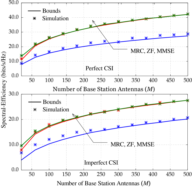
Figure 1: Lower bounds and numerically evaluated values of the spectral efficiency for different numbers of BS antennas for MRC, ZF, and MMSE with perfect and imperfect CSI. In this example there are $K=10$ users, the coherence interval $T=196$, the transmit power per terminal is $p_{\mathrm{u}}=10$ dB, and the propagation channel parameters were $\sigma_{\mathrm{shadow}}=8$ dB, and $\nu=3.8$.

We first conduct an experiment to validate the tightness of our proposed capacity bounds. Fig. 1 shows the simulated spectral efficiency and the proposed analytical bounds for MRC, ZF, and MMSE receivers with perfect and imperfect CSI at $p_{\mathrm{u}}=10$ dB. In this example there are $K=10$ users. For CSI estimation from uplink pilots, we choose pilot sequences of length $\tau=K$. (This is the smallest amount of training that can be used.) Clearly, all bounds are very tight, especially at large $M$. Therefore, in the following, we will use these bounds for all numerical work.

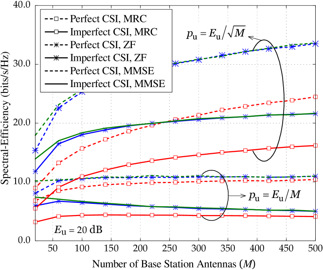
Figure 2: Spectral efficiency versus the number of BS antennas $M$ for MRC, ZF, and MMSE processing at the receiver, with perfect CSI and with imperfect CSI (obtained from uplink pilots). In this example $K=10$ users are served simultaneously, the reference transmit power is $E_{\mathrm{u}}=20$ dB, and the propagation parameters were $\sigma_{\mathrm{shadow}}=8$ dB and $\nu=3.8$.

We next illustrate the power scaling laws. Fig. 2 shows the spectral efficiency on the uplink versus the number of BS antennas for $p_{\mathrm{u}}=E_{\mathrm{u}}/M$ and $p_{\mathrm{u}}=E_{\mathrm{u}}/\sqrt{M}$ with perfect and imperfect receiver CSI, and with MRC, ZF, and MMSE processing, respectively. Here, we choose $E_{\mathrm{u}}=20$ dB. At this SNR, the spectral efficiency is in the order of 10–30 bits/s/Hz, corresponding to a spectral efficiency per user of 1–3 bits/s/Hz. These operating points are reasonable from a practical point of view. For example, 64-QAM with a rate-1/2 channel code would correspond to 3 bits/s/Hz. (Figure 3, see below, shows results at lower SNR.) As expected, with $p_{\mathrm{u}}=E_{\mathrm{u}}/M$, when $M$ increases, the spectral efficiency approaches a constant value for the case of perfect CSI, but decreases to $0$ for the case of imperfect CSI. However, with $p_{\mathrm{u}}=E_{\mathrm{u}}/\sqrt{M}$, for the case of perfect CSI the spectral efficiency grows without bound (logarithmically fast with $M$) when $M\to\infty$ and with imperfect CSI, the spectral efficiency converges to a nonzero limit as $M\to\infty$. These results confirm that we can scale down the transmitted power of each user as $E_{\mathrm{u}}/M$ for the perfect CSI case, and as $E_{\mathrm{u}}/\sqrt{M}$ for the imperfect CSI case when $M$ is large.

Typically ZF is better than MRC at high SNR, and vice versa at low SNR [14]. MMSE always performs the best across the entire SNR range (see Remark 1). When comparing MRC and ZF in Fig. 2, we see that here, when the transmitted power is proportional to $1/\sqrt{M}$, the power is not low enough to make MRC perform as well as ZF. But when the transmitted power is proportional to $1/M$, MRC performs almost as well as ZF for large $M$. Furthermore, as we can see from the figure, MMSE is always better than MRC or ZF, and its performance is very close to ZF.

In Fig. 3, we consider the same setting as in Fig. 2, but we choose $E_{\mathrm{u}}=5$ dB. This figure provides the same insights as Fig. 2. The gap between the performance of MRC and that of ZF (or MMSE) is reduced compared with Fig. 2. This is so because the relative effect of crosstalk interference (the interference from other users) as compared to the thermal noise is smaller here than in Fig. 2.

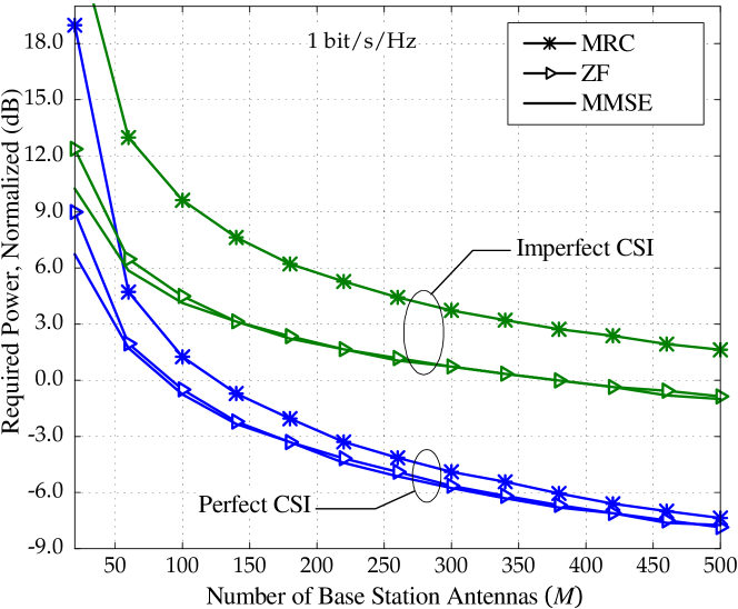
Figure 4: Transmit power required to achieve $1$ bit/channel use per user for MRC, ZF, and MMSE processing, with perfect and imperfect CSI, as a function of the number $M$ of BS antennas. The number of users is fixed to $K=10$, and the propagation parameters are $\sigma_{\mathrm{shadow}}=8$ dB and $\nu=3.8$.

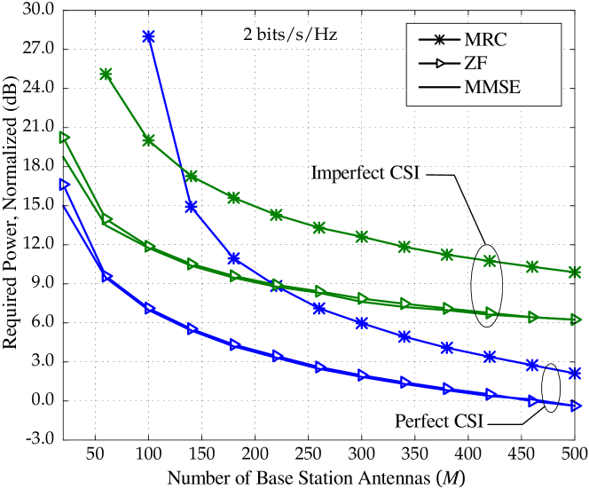
Figure 5: Same as Figure 4 but for a target spectral efficiency of 2 bits/channel use per user.

We next show the transmit power per user that is needed to reach a fixed spectral efficiency. Fig. 4 shows the normalized power ($p_{\mathrm{u}}$) required to achieve $1$ bit/s/Hz per user as a function of $M$. As predicted by the analysis, by doubling $M$, we can cut back the power by approximately 3 dB and 1.5 dB for the cases of perfect and imperfect CSI, respectively. When $M$ is large ($M/K\gtrapprox 6$), the difference in performance between MRC and ZF (or MMSE) is less than $1$ dB and $3$ dB for the cases of perfect and imperfect CSI, respectively. This difference increases when we increase the target spectral efficiency. Fig. 5 shows the normalized power required for $2$ bit/s/Hz per user. Here, the crosstalk interference is more significant (relative to the thermal noise) and hence the ZF and MMSE receivers perform relatively better.

V-A2 Energy Efficiency versus Spectral Efficiency Tradeoff

We next examine the tradeoff between energy efficiency and spectral efficiency in more detail. Here, we ignore the effect of large-scale fading, i.e., we set ${\boldsymbol{D}}={\boldsymbol{I}}_{K}$. We normalize the energy efficiency against a reference mode corresponding to a single-antenna BS serving one single-antenna user with $p_{\mathrm{u}}=10$ dB. For this reference mode, the spectral efficiencies and energy efficiencies for MRC, ZF, and MMSE are equal, and given by (from (42) and (66))

$$R_{\mathrm{IP}}^{0}=\frac{T-\tau}{T}\operatorname{\mathbb{E}}\left\{\log_{2}\left(1+\frac{\tau p_{\mathrm{u}}^{2}|z|^{2}}{1+p_{\mathrm{u}}\left(1+\tau\right)}\right)\right\},~{}\eta_{\mathrm{IP}}^{0}=R_{\mathrm{IP}}^{0}/p_{\mathrm{u}}$$

where $z$ is a Gaussian RV with zero mean and unit variance. For the reference mode, the spectral-efficiency is obtained by choosing the duration of the uplink pilot sequence $\tau$ to maximize $R_{\mathrm{IP}}^{0}$. Numerically we find that $R_{\mathrm{IP}}^{0}=2.65$ bits/s/Hz and $\eta_{\mathrm{IP}}^{0}=0.265$ bits/J.

Fig. 6 shows the relative energy efficiency versus the the spectral efficiency for MRC and ZF. The relative energy efficiency is obtained by normalizing the energy efficiency by $\eta_{\mathrm{IP}}^{0}$ and it is therefore dimensionless. The dotted and dashed lines show the performances for the cases of $M=1,K=1$ and $M=100,K=1$, respectively. Each point on the curves is obtained by choosing the transmit power $p_{\mathrm{u}}$ and pilot sequence length $\tau$ to maximize the energy efficiency for a given spectral efficiency. The solid lines show the performance for the cases of $M=50$, and $100$. Each point on these curves is computed by jointly choosing $K$, $\tau$, and $p_{\mathrm{u}}$ to maximize the energy-efficiency subject a fixed spectral-efficiency, i.e.,

$$\arg\mathop{\max}\limits_{p_{\mathrm{u}},K,\tau}~{}\eta_{\mathrm{IP}}^{\tt A},\hskip 28.45274pt\text{s.t.}~{}R_{\mathrm{IP}}^{\tt A}=\text{const.},K\leq\tau\leq T$$

We first consider a single-user system with $K=1$. We compare the performance of the cases $M=1$ and $M=100$. Since $K=1$ the performances of MRC and ZF are equal. With the same power used as in the reference mode, i.e., $p_{\mathrm{u}}=10$ dB, using $100$ antennas can increase the spectral efficiency and the energy efficiency by factors of $4$ and $3$, respectively. Reducing the transmit power by a factor of $100$, from $10$ dB to $-10$ dB yields a $100$-fold improvement in energy efficiency compared with that of the reference mode with no reduction in spectral-efficiency.

We next consider a multiuser system ($K>1$). Here the transmit power $p_{\mathrm{u}}$, the number of users $K$, and the duration of pilot sequences $\tau$ are chosen optimally for fixed $M$. We consider $M=50$ and $100$. Here the system performance improves very significantly compared to the single-user case. For example, with MRC, at $p_{\mathrm{u}}=0$ dB, compared with the case of $M=1,K=1$, the spectral-efficiency increases by factors of $50$ and $80$, while the energy-efficiency increases by factors of $55$ and $75$ for $M=50$ and $M=100$, respectively. As discussed in Section IV, at low spectral efficiency, the energy efficiency increases when the spectral efficiency increases. Furthermore, we can see that at high spectral efficiency, ZF outperforms MRC. This is due to the fact that the MRC receiver is limited by the intracell interference, which is significant at high spectral efficiency. As a consequence, when $p_{\mathrm{u}}$ is increased, the spectral efficiency of MRC approaches a constant value, while the energy efficiency goes to zero (see (70)).

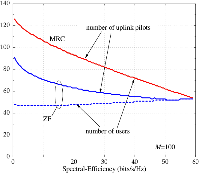
Figure 7: Optimal number of users $K$ and number of symbols $\tau$ spent on training, out of a total of $T=196$ symbols per coherence interval, for the curves in Fig. 6 corresponding to $M=100$ antennas.

The corresponding optimum values of $K$ and $\tau$ as functions of the spectral efficiency for $M=100$ are shown in Fig. 7. For MRC, the optimal number of users and uplink pilots are the same (this means that the minimal possible length of training sequences are used). For ZF, more of the coherence interval is used for training. Generally, at low transmit power and therefore at low spectral efficiency, we spend more time on training than on payload data transmission. At high power (high spectral efficiency and low energy efficiency), we can serve around $55$ users, and $K=\tau$ for both MRC and ZF.

V-B Multicell MU-MIMO Systems

Next, we examine the effect of pilot contamination on the energy and spectral efficiency for multicell systems. We consider a system with $L=7$ cells. Each cell has the same size as in the single-cell system. When shrinking the cell size, one typically also cuts back on the power. Hence, the relation between signal and interference power would not be substantially different in systems with smaller cells and in that sense, the analysis is largely independent of the actual physical size of the cell [24]. Note that, setting $L=7$ means that we consider the performance of a given cell with the interference from $6$ nearest-neighbor cells. We assume ${\boldsymbol{D}}_{ll}={\boldsymbol{I}}_{K}$, and ${\boldsymbol{D}}_{li}=\beta{\boldsymbol{I}}_{K}$, for $i\neq l$. To examine the performance in a practical scenario, the intercell interference factor, $\beta$, is chosen as follows. We consider two users, the $1$st user is located uniformly at random in the first cell, and the $2$nd user is located uniformly at random in one of the $6$ nearest-neighbor cells of the $1$st cell. Let $\bar{\beta}_{1}$ and $\bar{\beta}_{2}$ be the large scale fading from the $1$st user and the $2$nd user to the $1$st BS, respectively. (The large scale fading is modelled as in Section V-A1.) Then we compute $\beta$ as $\operatorname{\mathbb{E}}\left\{\bar{\beta}_{2}/\bar{\beta}_{1}\right\}$. By simulation, we obtain $\beta=0.32,0.11$, and $0.04$ for the cases of ($\sigma_{\mathrm{shadow}}=8$ dB, $\nu=3.8,f_{\mathrm{reuse}}=1$), ($\sigma_{\mathrm{shadow}}=8$ dB, $\nu=3,f_{\mathrm{reuse}}=1$), and ($\sigma_{\mathrm{shadow}}=8$ dB, $\nu=3.8,f_{\mathrm{reuse}}=3$), respectively, where $f_{\mathrm{reuse}}$ is the frequency reuse factor.

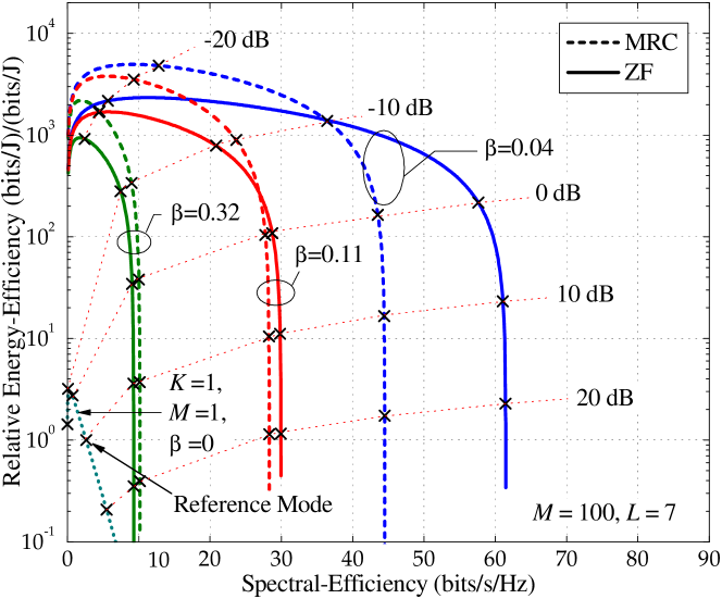
Figure 8: Same as Figure 6, but for a multicell scenario, with $L=7$ cells, and coherence interval $T=196$.

Fig. 8 shows the relative energy efficiency versus the spectral efficiency for MRC and ZF of the multicell system. The reference mode is the same as the one in Fig. 6 for a single-cell system. The dotted line shows the performance for the case of $M=1,K=1$, and $\beta=0$. The solid and dashed lines show the performance for the cases of $M=100$, and $L=7$, with different intercell interference factors $\beta$ of $0.32,0.11$, and $0.04$. Each point on these curves is computed by jointly choosing $\tau$, $K$, and $p_{\mathrm{u}}$ to maximize the energy efficiency for a given spectral efficiency. We can see that the pilot contamination significantly degrades the system performance. For example, when $\beta$ increases from $0.11$ to $0.32$ (and hence, the pilot contamination increases), with the same power, $p_{\mathrm{u}}=10$ dB, the spectral efficiency and the energy efficiency reduce by factors of $3$ and $2.7$, respectively. However, with low transmit power where the spectral efficiency is smaller than $10$ bits/s/Hz, the system performance is not affected much by the pilot contamination. Furthermore, we can see that in a multicell scenario with high pilot contamination, MRC achieves a better performance than ZF.

VI Conclusion

Very large MIMO systems offer the opportunity of increasing the spectral efficiency (in terms of bits/s/Hz sum-rate in a given cell) by one or two orders of magnitude, and simultaneously improving the energy efficiency (in terms of bits/J) by three orders of magnitude. This is possible with simple linear processing such as MRC or ZF at the BS, and using channel estimates obtained from uplink pilots even in a high mobility environment where half of the channel coherence interval is used for training. Generally, ZF outperforms MRC owing to its ability to cancel intracell interference. However, in multicell environments with strong pilot contamination, this advantage tends to diminish. MRC has the additional benefit of facilitating a distributed per-antenna implementation of the detector. These conclusions are valid in an operating regime where $100$ antennas serve about $50$ terminals in the same time-frequency resource, each terminal having a fading-free throughput of about $1$ bpcu, and hence the system offering a sum-throughput of about $50$ bpcu.

-A Proof of Proposition 2

From (19), we have

$$\tilde{R}_{\mathrm{P},k}^{\tt{mrc}}=\log_{2}\left(1+\left(\operatorname{\mathbb{E}}\left\{\frac{p_{\mathrm{u}}\sum_{i=1,i\neq k}^{K}|\tilde{g}_{i}|^{2}+1}{p_{\mathrm{u}}\|{\boldsymbol{g}}_{k}\|^{2}}\right\}\right)^{-1}\right)$$ (79)

where $\tilde{g}_{i}\triangleq\frac{{\boldsymbol{g}}_{k}^{H}{\boldsymbol{g}}_{i}}{\|{\boldsymbol{g}}_{k}\|}$. Conditioned on ${\boldsymbol{g}}_{k}$, $\tilde{g}_{i}$ is a Gaussian RV with zero mean and variance $\beta_{i}$ which does not depend on ${\boldsymbol{g}}_{k}$. Therefore, $\tilde{g}_{i}$ is Gaussian distributed and independent of ${\boldsymbol{g}}_{k}$, $\tilde{g}_{i}\sim\mathcal{CN}\left({0},{\beta_{i}}\right)$. Then,

$$\operatorname{\mathbb{E}}\left\{\frac{p_{\mathrm{u}}\sum_{i=1,i\neq k}^{K}|\tilde{g}_{i}|^{2}+1}{p_{\mathrm{u}}\|{\boldsymbol{g}}_{k}\|^{2}}\right\} =\left(p_{\mathrm{u}}\sum_{i=1,i\neq k}^{K}\operatorname{\mathbb{E}}\left\{|\tilde{g}_{i}|^{2}\right\}+1\right)\operatorname{\mathbb{E}}\left\{\frac{1}{p_{\mathrm{u}}\|{\boldsymbol{g}}_{k}\|^{2}}\right\}$$

$$=\left(p_{\mathrm{u}}\sum_{i=1,i\neq k}^{K}\beta_{i}+1\right)\operatorname{\mathbb{E}}\left\{\frac{1}{p_{\mathrm{u}}\|{\boldsymbol{g}}_{k}\|^{2}}\right\}$$ (80)

Using the identity [23]

$$\operatorname{\mathbb{E}}\left\{{\tt tr}\left({\boldsymbol{W}}^{-1}\right)\right\}=\frac{m}{n-m}$$ (81)

where ${\boldsymbol{W}}\sim\mathcal{W}_{m}\left(n,{\boldsymbol{I}}_{n}\right)$ is an $m\times m$ central complex Wishart matrix with $n$ ($n>m$) degrees of freedom, we obtain

$$\operatorname{\mathbb{E}}\left\{\frac{1}{p_{\mathrm{u}}\|{\boldsymbol{g}}_{k}\|^{2}}\right\} =\frac{1}{p_{\mathrm{u}}\left(M-1\right)\beta_{k}},~{}\text{for $M\geq 2$}$$ (82)

Substituting (82) into (-A), we arrive at the desired result (20).

-B Proof of Proposition 3

From (3), we have

$$\operatorname{\mathbb{E}}\left\{\left[\left({\boldsymbol{G}}^{H}{\boldsymbol{G}}\right)^{-1}\right]_{kk}\right\} =\frac{1}{\beta_{k}}\operatorname{\mathbb{E}}\left\{\left[\left({\boldsymbol{H}}^{H}{\boldsymbol{H}}\right)^{-1}\right]_{kk}\right\}=\frac{1}{K\beta_{k}}\operatorname{\mathbb{E}}\left\{{\tt tr}\left[\left({\boldsymbol{H}}^{H}{\boldsymbol{H}}\right)^{-1}\right]\right\}$$

$$\mathop{=}\limits^{(a)}\frac{1}{\left(M-K\right)\beta_{k}},~{}\text{for $M\geq K+1$}$$ (83)

where $(a)$ is obtained by using (81). Using (-B), we get (24).

TABLE I: Lower bounds on the achievable rates of the uplink transmission for the $k$th user.

Perfect CSI Imperfect CSI MRC $\log_{2}\left(1+\frac{p_{\mathrm{u}}\left(M-1\right)\beta_{k}}{p_{\mathrm{u}}\sum_{i=1,i\neq k}^{K}\beta_{i}+1}\right)$ $\log_{2}\left(1+\frac{\tau p_{\mathrm{u}}^{2}\left(M-1\right)\beta_{k}^{2}}{p_{\mathrm{u}}\left(\tau p_{\mathrm{u}}\beta_{k}+1\right)\sum_{i=1,i\neq k}^{K}\beta_{i}+\left(\tau+1\right)p_{\mathrm{u}}\beta_{k}+1}\right)$ ZF $\log_{2}\left(1+p_{\mathrm{u}}\left(M-K\right)\beta_{k}\right)$ $\log_{2}\left(1+\frac{\tau p_{\mathrm{u}}^{2}\left(M-K\right)\beta_{k}^{2}}{\left(\tau p_{\mathrm{u}}\beta_{k}+1\right)\sum_{i=1}^{K}\frac{p_{\mathrm{u}}\beta_{i}}{\tau p_{\mathrm{u}}\beta_{i}+1}+\tau p_{\mathrm{u}}\beta_{k}+1}\right)$ MMSE $\log_{2}\left(1+\left(\alpha_{k}-1\right)\theta_{k}\right)$ $\log_{2}\left(1+\left(\hat{\alpha}_{k}-1\right)\hat{\theta}_{k}\right)$

Figure 3: Same as Figure 2, but with $E_{\mathrm{u}}=5$ dB.

Figure 6: Energy efficiency (normalized with respect to the reference mode) versus spectral efficiency for MRC and ZF receiver processing with imperfect CSI. The reference mode corresponds to $K=1,M=1$ (single antenna, single user), and a transmit power of $p_{\mathrm{u}}=10$ dB. The coherence interval is $T=196$ symbols. For the dashed curves (marked with $K=1$), the transmit power $p_{\mathrm{u}}$ and the fraction of the coherence interval $\tau/T$ spent on training was optimized in order to maximize the energy efficiency for a fixed spectral efficiency. For the green and red curves (marked MRC and ZF; shown for $M=50$ and $M=100$ antennas, respectively), the number of users $K$ was optimized jointly with $p_{\mathrm{u}}$ and $\tau/T$ to maximize the energy efficiency for given spectral efficiency. Any operating point on the curves can be obtained by appropriately selecting $p_{\mathrm{u}}$ and optimizing with respect to $K$ and $\tau/T$. The number marked next to the $\times$ marks on each curve is the power $p_{\mathrm{u}}$ spent by the transmitter.

References

• [1]
• [2] H. Q. Ngo, E. G. Larsson, and T. L. Marzetta, “Uplink power efficiency of multiuser MIMO with very large antenna arrays,” in Proc. Allerton Conf. Commun., Control, Comput., Urbana-Champaign, IL., Sept. 2011, pp.1272-1279.
• [3] D. Gesbert, M. Kountouris, R. W. Heath Jr., C.-B. Chae, and T. Sälzer, “Shifting the MIMO paradigm,” IEEE Sig. Proc. Mag., vol. 24, no. 5, pp. 36–46, 2007.
• [4] G. Caire, N. Jindal, M. Kobayashi, and N. Ravindran, “Multiuser MIMO achievable rates with downlink training and channel state feedback,” IEEE Trans. Inf. Theory, vol. 56, no. 6, pp. 2845–2866, 2010.
• [5] J. Jose, A. Ashikhmin, T. L. Marzetta, and S. Vishwanath, “Pilot contamination and precoding in multi-cell TDD systems,” IEEE Trans. Wireless Commun., vol. 10, no. 8, pp. 2640–2651, Aug. 2011.
• [6] S. Verdú, Multiuser Detection, Cambridge University Press, 1998.
• [7] P. Viswanath and D. N. C. Tse, “Sum capacity of the vector Gaussian broadcast channel and uplink-downlink duality” IEEE Trans. Inf. Theory, vol. 49, no. 8, pp. 1912–1921, Aug. 2003.
• [8] H. Weingarten, Y. Steinberg, and S. Shamai, “The capacity region of the Gaussian multiple-input multiple-output broadcast channel,” IEEE Trans. Inf. Theory, vol. 52, no. 9, pp. 3936–3964, Sep. 2006.
• [9] T. L. Marzetta, “Noncooperative cellular wireless with unlimited numbers of BS antennas,” IEEE Trans. Wireless Commun., vol. 9, no. 11, pp. 3590–3600, Nov. 2010.
• [10] ——, “How much training is required for multiuser MIMO,” in Fortieth Asilomar Conference on Signals, Systems and Computers (ACSSC ’06), Pacific Grove, CA, USA, Oct. 2006, pp. 359–363.
• [11] F. Rusek, D. Persson, B. K. Lau, E. G. Larsson, T. L. Marzetta, O. Edfors, and F. Tufvesson, “Scaling up MIMO: Opportunities and challenges with very large arrays,” IEEE Sig. Proc. Mag., accepted. [Online]. Available: arxiv.org/abs/1201.3210.
• [12] J. Hoydis, S. ten Brink, and M. Debbah, “Massive MIMO: How many antennas do we need?,” in Proc. 49th Allerton Conference on Communication, Control, and Computing, 2011.
• [13] A. Fehske, G. Fettweis, J. Malmodin and G. Biczok, “The global footprint of mobile communications: the ecological and economic perspective,” IEEE Communications Magazine, pp. 55-62, August 2011.
• [14] D. N. C. Tse and P. Viswanath, Fundamentals of Wireless Communications.   Cambridge, UK: Cambridge University Press, 2005.
• [15] H. Huh, G. Caire, H. C. Papadopoulos, S. A. Rampshad, “Achieving large spectral efficiency with TDD and not-so-many base station antennas,” in Proc. IEEE Antennas and Propagation in Wireless Communications (APWC), 2011.
• [16] S. Wagner, R. Couillet, D. T. M. Slock, and M. Debbah, “Large system analysis of zero-forcing precoding in MISO broadcast channels with limited feedback,” in Proc. IEEE Int. Works. Signal Process. Adv. Wireless Commun. (SPAWC), 2010.
• [17] H. Yang and T. L. Marzetta, “Performance of conjugate and zero-forcing beanforming in large-scale antenna systems”, IEEE J. Select. Areas Commun., 2012, submitted.
• [18] H. Cramér, Random Variables and Probability Distributions.   Cambridge, UK: Cambridge University Press, 1970.
• [19] N. Kim and H. Park, “Performance analysis of MIMO system with linear MMSE receiver,” IEEE Trans. Wireless Commun., vol. 7, no. 11, pp. 4474–4478, Nov. 2008.
• [20] H. Gao, P. J. Smith, and M. Clark, “Theoretical reliability of MMSE linear diversity combining in Rayleigh-fading additive interference channels,” IEEE Trans. Commun., vol. 46, no. 5, pp. 666–672, May 1998.
• [21] P. Li, D. Paul, R. Narasimhan, and J. Cioffi, “On the distribution of SINR for the MMSE MIMO receiver and performance analysis,” IEEE Trans. Inf. Theory, vol. 52, no. 1, pp. 271–286, Jan. 2006.
• [22] I. S. Gradshteyn and I. M. Ryzhik, Table of Integrals, Series, and Products, 7th ed.   San Diego, CA: Academic, 2007.
• [23] A. M. Tulino and S. Verdú, “Random matrix theory and wireless communications,” Foundations and Trends in Communications and Information Theory, vol. 1, no. 1, pp. 1–182, Jun. 2004.
• [24] A. Lozano, R. W. Heath Jr., and J. G. Andrews, “Fundamentral limits of cooperation,” Mar. 2012. [Online]. Available: arxiv.org/abs/1204.0011.