Differential cross section and analysing power of the quasi-free $pn\to\{pp\}_{s}\pi^{-}$ reaction at 353 MeV

Abstract

In order to establish links between $p$-wave pion production in nucleon-nucleon collisions and low energy three-nucleon scattering, an extensive programme of experiments on pion production is currently underway at COSY-ANKE. The final proton pair is measured at very low excitation energy, leading to an $S$-wave diproton, denoted here as $\{pp\}_{\!s}$. By using a deuterium target we have obtained data on the differential cross section and analysing power of the quasi-free $\pol{p}n\to\{pp\}_{s}\pi^{-}$ reaction at 353 MeV. The spectator proton $p_{\rm sp}$ was either measured directly in silicon tracking telescopes or reconstructed using the momentum of a detected $\pi^{-}$. Both observables can be described in terms of $s$-, $p$-, and $d$-wave pion production amplitudes. Taken together with the analogous data on the $\pol{p}p\to\{pp\}_{\!s\,}\pi^{0}$ reaction, full partial wave decompositions of both processes were carried out.

, , , , , , , , , , , , , , , , , , , , , , , , , , , , , , , , , , , , , ,

There is an extensive programme of near-threshold measurements of $NN\to\{pp\}_{\!s\,}\pi$ at the COSY-ANKE facility of the Forschungszentrum Jülich [1, 2]. Here the $\{pp\}_{\!s}$ denotes a proton-proton system with very low excitation energy, $E_{pp}$, which is overwhelmingly in the ${}^{1\!}S_{0}$ state with antiparallel proton spins. The primary aim of these experiments is to carry out a full amplitude analysis which would lead to a determination of the pion $p$-wave production strength from the ${}^{3\!}S_{1}$ initial state that could provide links with other intermediate energy phenomena. As part of this programme, we have already presented data on the cross section and analysing power of the $\pol{p}p\to\{pp\}_{\!s\,}\pi^{0}$ reaction, which can be described in terms of $s$- and $d$-wave pion production amplitudes [3]. We here present analogous results for the quasi-free $\pol{p}n\to\{pp\}_{s}\pi^{-}$ reaction at an effective beam energy around 353 MeV.

In the absence of an intense monochromatic neutron beam, the study of the $pn\to\{pp\}_{s}\pi^{-}$ reaction is most easily carried out through quasi-free $\pi^{-}$ production, with a proton beam incident on a deuterium target. In order to make a full reconstruction of a $pd\to p_{\rm sp}\{pp\}_{\!s\,}\pi^{-}$ event, it is necessary to measure accurately the momentum of three of the particles in the final state. Determinations have been made at TRIUMF of both the cross section [4] and proton analysing power [5] by detecting the pion together with the two fast protons. The spectator proton, $p_{\rm sp}$, was then identified through the missing mass in the reaction and its momentum reconstructed kinematically. Data were taken for three beam energies, though only in the central region of pion angles. The lowest of these energies was 353 MeV and, to allow a close comparison, we have concentrated our attention on this energy.

In contrast to the TRIUMF data, we have extended the coverage to the whole angular domain, which is very important in the subsequent partial wave analysis. Furthermore, by including the possibility of detecting directly the spectator proton or the $\pi^{-}$, we have obtained an independent check on some of the systematics involved.

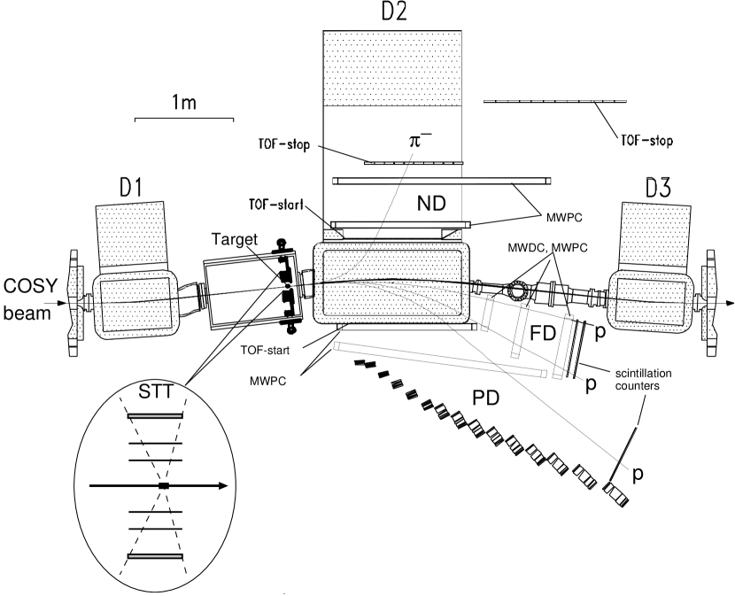
Figure 1: Top view of the ANKE spectrometer setup, showing the positions of the Positive (PD), Negative (ND), and Forward (FD) detectors, as well as the Silicon Tracking Telescope (STT). The dipoles D1 and D3 deflect the circulating proton beam in and out of ANKE, whereas D2 serves as an analysing magnet.

The experiment was carried out at the ANKE spectrometer facility [6], which is installed inside the COSY cooler synchrotron storage ring of the Forschungszentrum Jülich. The circulating proton beam was polarised perpendicularly to the horizontal plane of the machine and the polarisation reversed in direction every six minutes.

Fast protons arising from the interaction of the beam with the deuterium cluster-jet target [7] traversed the spectrometer dipole magnet D2 shown in Fig. 1 and entered the forward (FD) and/or positive side (PD) detectors. Negative pions produced in the interaction at small centre-of-mass (CM) angles, $\theta_{\pi}<40^{\circ}$, could be detected in the negative side detector (ND), while slow spectator protons ($p_{\rm sp}$) were observed in one of the silicon tracking telescopes (STT) that were located in the target vacuum chamber close to the target jet [8, 9].

Each of the FD, PD, and ND detectors shown in Fig. 1 includes both scintillation counters and multiwire proportional (MWPC) or drift chambers (MWDC). The reconstruction of the particle trajectories from hits in the wire chambers allowed the momenta of the ejectiles to be evaluated. The counters were used to measure the arrival times and energy losses required for particle identification.

The two STT were placed symmetrically to the left and right of the target jet. Each telescope consists of three sensitive silicon layers, though only the first two were used in this experiment. Spectator protons with the energies $2.5<E_{\rm sp}<6$ MeV pass through the first layer and stop in the second. The accuracy of the energy measurement, $\sigma(E_{\rm sp})/E_{\rm sp}\simeq 10\%$, allow protons to be identified by their energy loss [10]. Although higher energy recoil protons could be measured by using the third STT layer, to stay within the range of applicability of the spectator model, only events with $E_{\rm{sp}}<6$ MeV were retained. It should, however, be noted that there is no lower limit on $E_{\rm{sp}}$ when the $\pi^{-}$ is measured.

In order to provide sufficient resolution in $E_{pp}$, both fast protons from the diproton have to be detected and, to permit a complete reconstruction of the kinematics of the reaction, one has in addition to detect either the $\pi^{-}$ or the slow spectator proton. The triggers selected fast proton pairs, with either both protons hitting the FD or PD, or one proton recorded in each detector. A trigger for single tracks in the FD was also added to record deuterons from the $pn\to d\pi^{0}$ process, which were used for normalisation and polarimetry purposes. A sample of data was also taken with a special trigger requiring a coincidence between the first two layers of the STT. This was used to investigate the STT performance and for background studies.

The CM energy of the quasi-free $pn$ system depends on the energy and the emission angle of the spectator and for this experiment the effective “free” beam energy was in the range $T_{\rm{free}}\approx(310$–$390)$ MeV. However, for the reconstructed events, $T_{\rm{free}}$ was measured with an accuracy of $\sigma(T_{\rm{free}})=2$–$4$ MeV and only data in the range $T_{\rm{free}}=353\pm 20$ MeV were used in the analysis.

The identification of the $pd\to p_{\rm sp}\{pp\}_{\!s\,}\pi^{-}$ reaction starts from the selection of pairs of fast protons through the difference between their times of flights in ANKE [11]. Since the beam energy is quite low, other pairs of particles gave a negligible contribution to the background, which originated mostly from accidental coincidences, and amounted to $\lesssim 7\%$. To select the ${}^{1\!}S_{0}$ diproton state, we imposed a $E_{pp}<3$ MeV cut on the data, which could be done reliably because of the excellent resolution of $\sigma(E_{pp})<0.6$ MeV. It is important to note that the identical cut was placed on the $pp\to\{pp\}_{\!s\,}\pi^{0}$ data [3], which is important when considering the relative normalisation uncertainties for $\pi^{0}$ and $\pi^{-}$ production.

The time-of-flight criterion was also used to select the $\pi^{-}$ in the ND, where the very low background consisted only of accidentals and strongly scattered positively charged particles. The background level for the spectator protons identified in the STT was at the 5–8% level, depending on the proton energy and angle.

Having measured three of the final particles, the residual one from the $pd\to p_{\rm sp}\{pp\}_{\!s\,}\pi^{-}$ reaction was identified by the missing-mass method. This is illustrated separately in Fig. 2 for the cases where the spectator proton or $\pi^{-}$ was detected. The main backgrounds were from accidental coincidences, which were particularly significant for spectator protons because no timing information from the STT was used in the analysis. The shape of this background was derived from artificially constructed events. The momenta of the fast protons were taken from the experimental events where neither a spectator proton nor $\pi^{-}$ was detected, to which was added a random spectator momentum taken from the sample acquired with the STT trigger. The missing-mass spectrum was then fitted with the sum of this background distribution and a Gaussian. The background level was estimated separately for each detector combination, spin orientation of the beam, and angular bin. Any uncertainties here were combined with the statistical errors.

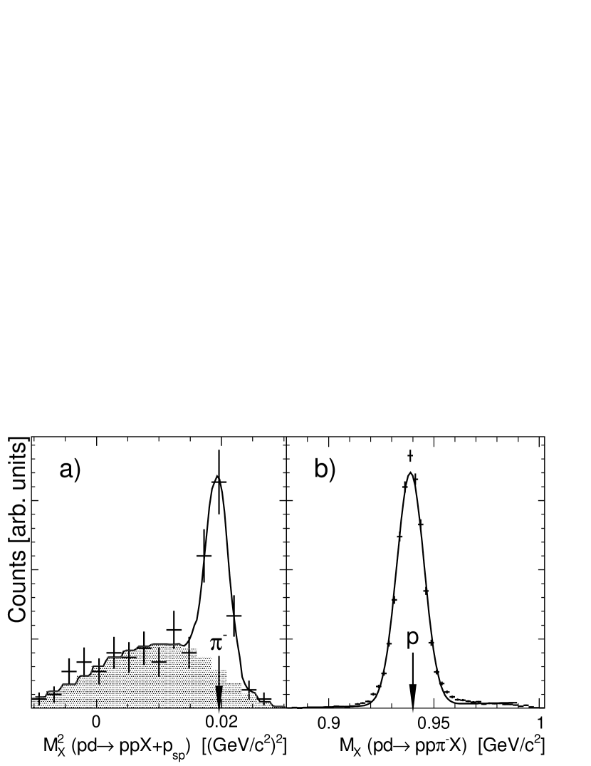
Figure 2: Kinematic identification of the $pd\to p_{\rm sp}\{pp\}_{\!s\,}\pi^{-}$ reaction. a) Sample of missing-mass squared data from events where the spectator proton is detected, showing the experimental spectrum (with error bars), the background (shaded area), and the sum of this plus a Gaussian for the $\pi^{-}$ peak (solid curve). b) Missing-mass distribution when the $\pi^{-}$ is detected. The curve shows the fit to the experimental data with the sum of a Gaussian centred on the mass of the proton and a linear background.

In order to estimate the resolutions and acceptance of the system, a full simulation of the ANKE setup was performed [11], based on the GEANT package [12]. The acceptance was calculated as a function of $\theta_{\pi}$ for both the $\pi^{-}$ and spectator proton detection, assuming that the spectator was emitted isotropically, with the energy being sampled from the Fermi distribution [13]. The fast proton pair was generated in the ${}^{1\!}S_{0}$ state, with the distribution in excitation energy being weighted by the Migdal-Watson factor [14] that included the Coulomb interaction [15].

The polarisation of the proton beam and the luminosity were both estimated from quasi-free $\pol{p}n\to d\pi^{0}$ data that were taken in parallel. The fast deuteron was detected in the FD, and selected by its energy loss in the counters, and the spectator proton measured in coincidence in the STT. The reaction was then identified by the missing-mass method.

The measurements of both the analysing power and cross section depend sensitively on the relative luminosities for the two spin states and this was controlled by comparing the rates of ejectiles emitted at $\theta=0^{\circ}$ or $\phi=\pm 90^{\circ}$, which cannot depend upon the beam polarisation. Using calibration data taken from the SAID database [16], the integrated luminosity was found to be $L=(2310\pm 110)~{}\textrm{nb}^{-1}$. No correction was made for the shadowing in the deuteron since there is a similar effect in the measurement of the quasi-free $pn\to\{pp\}_{s}\pi^{-}$ rate. The beam polarisation determined in this way was $P=0.66\pm 0.06$. This is consistent with that found in the $\pi^{0}$ production experiment [3] that was undertaken with the same conditions just before the $\pi^{-}$ run. The luminosities in the two polarisation states were on average very close, $L_{\uparrow}/L_{\downarrow}=1.017\pm 0.005$.

Figure 3 shows the differential cross-section $d\sigma/d\Omega$ for the quasi-free $pn\to\{pp\}_{s}\pi^{-}$ reaction integrated over the $E_{pp}=(0-3)$ MeV range of $pp$ excitation energies and averaged over the effective beam energy $T_{\rm{free}}=353\pm 20$ MeV. The data were extracted within the impulse approximation model, where the weighting of the spectator momentum distribution was taken from the Bonn deuteron wave function [17], though the result was insensitive to this choice. The cross-section was estimated separately for $\pi^{-}$ and spectator proton detection and, since these two results were found to be consistent, only their weighted average is presented. Also shown are the TRIUMF data on quasi-free $\pi^{-}$ production [4]. They imposed a slightly more severe $E_{pp}$ cut on their data and these were converted to our 3 MeV cut by assuming a Migdal-Watson energy variation [14].

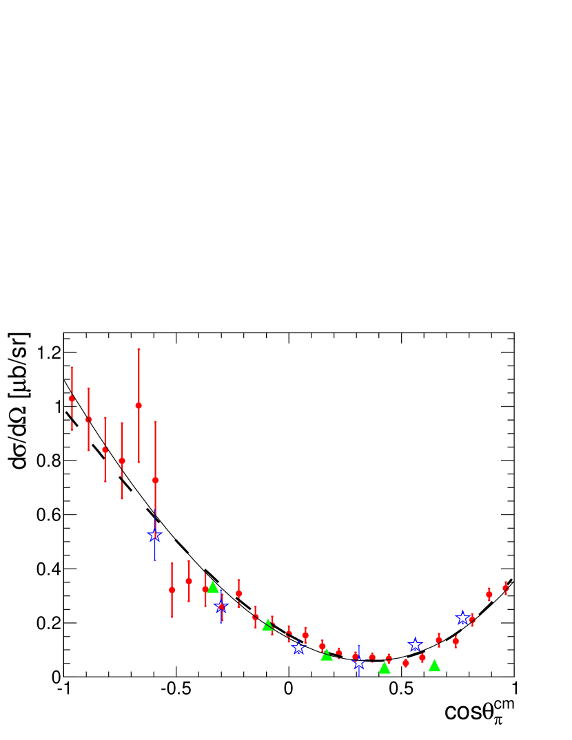
Figure 3: Unpolarised differential cross section for the $pn\to\{pp\}_{s}\pi^{-}$ reaction at $T_{\rm free}\approx 353$ MeV. The ANKE data with statistical errors are shown by red circles. In addition there is a systematic error of 6% arising from the luminosity and acceptance determination. The statistical errors of the TRIUMF $pn\to\{pp\}_{s}\pi^{-}$ results [4] (green triangles) are generally smaller than the symbol size and their normalisation uncertainty is 10%. The arbitrarily scaled TRIUMF cross sections extracted from $\pi^{-}{}^{3}\textrm{He}\to pnn_{\rm sp}$ data [18] (blue stars) are also included. The dashed curve is a direct cubic fit to these ANKE data whereas the solid one corresponds to the global fit described in the text.

Whereas the TRIUMF results only cover the central region of pion angles [4], the current data extend over the whole angular domain. The two data sets are consistent in the backward hemisphere but the TRIUMF measurements show no indication of the rise at forward angles that is seen at ANKE. Some confirmation of the ANKE angular shape is offered by pion absorption data, $\pi^{-}{}^{3}\textrm{He}\to pnn_{\rm sp}$, where the unobserved slow neutron is assumed to be a spectator [18]. In this case the reaction can be interpreted as being $\pi^{-}\{pp\}_{\!s}\to pn$, though the internal structure of the diproton is very different to that in the production data. Over the range of angles covered, our data are completely consistent with these absorption results. The forward/backward peaking is in complete contrast to the results found for $\pi^{0}$ production [20, 3] and is an indication of the dominance of the $I=0$ $p$-wave amplitudes in this reaction.

The unpolarised cross section for $\pi^{-}$ production, and this times the proton analysing power $A_{y}$, must be of the form

$$\left(\frac{d\sigma}{d\Omega}\right)_{\!0} = \frac{k}{4p}\sum_{n=0}a_{n}\cos^{n}\theta_{\pi},$$ (1)

$$A_{y}\left(\frac{d\sigma}{d\Omega}\right)_{\!0} = \frac{k}{4p}\sin\theta_{\pi}\sum_{n=0}b_{n+1}\cos^{n}\theta_{\pi},$$ (2)

where $\theta_{\pi}$ is the pion c.m. production angle with respect to the direction of the polarised proton beam. Here $p$ is the incident c.m. momentum and $k$ that of the produced pion. We are neglecting here any small effects due to the mass differences and at 353 MeV; the momenta then have values $p=407$ MeV/$c$ and $k\approx 94$ MeV/$c$. The best fits of Eq. (1) to the differential cross section are found with the parameters quoted in Table 1.

Observable	Direct fit	Global fit
$a_{0}(pp)$	$\phantom{-}4.05\pm 0.08$	$\phantom{-}4.05\pm 0.08$
$a_{2}(pp)$	$-2.31\pm 0.14$	$-2.34\pm 0.14$
$b_{2}(pp)$	$\phantom{-}1.82\pm 0.10$	$\phantom{-}1.80\pm 0.10$
$a_{0}(pn)$	$\phantom{-}2.69\pm 0.18$	$\phantom{-}2.47\pm 0.08$
$a_{1}(pn)$	$-8.24\pm 0.51$	$-7.83\pm 0.45$
$a_{2}(pn)$	$\phantom{-}9.11\pm 0.70$	$\phantom{1}10.12\pm 0.41$
$a_{3}(pn)$	$\phantom{-}2.89\pm 0.90$	$\phantom{-}1.38\pm 0.27$
$b_{1}(pn)$	$\phantom{-}1.77\pm 0.14$	$\phantom{-}1.82\pm 0.13$
$b_{2}(pn)$	$-1.95\pm 0.50$	$-1.75\pm 0.36$
$b_{3}(pn)$	$-4.43\pm 0.70$	$-4.83\pm 0.27$

Table 1: Values of the parameters in $\mu$b/sr extracted by direct fits of Eqs. (1) and (2) to the $pp\to\{pp\}_{\!s\,}\pi^{0}$ and $pn\to\{pp\}_{s}\pi^{-}$ experimental data and those obtained on the basis of Eq. (5) from the amplitudes given in Eq. (6). The error bars are purely statistical. In the $\pi^{-}$ case there are systematic uncertainties of 6% in the cross section and 9% in the analysing powers.

The results for the analysing power of the $\pol{p}n\to\{pp\}_{s}\pi^{-}$ reaction are displayed in Fig. 4, with $A_{y}(d\sigma/d\Omega)$ being shown in panel a and $A_{y}$ in panel b. The agreement with the TRIUMF $A_{y}$ data [5] is reasonable at large angles and both show the strong and rather asymmetric oscillation in the central region. However, there are clear discrepancies for $\theta_{\pi}\lesssim 60^{\circ}$, as there are also for the cross section shown in Fig. 3.

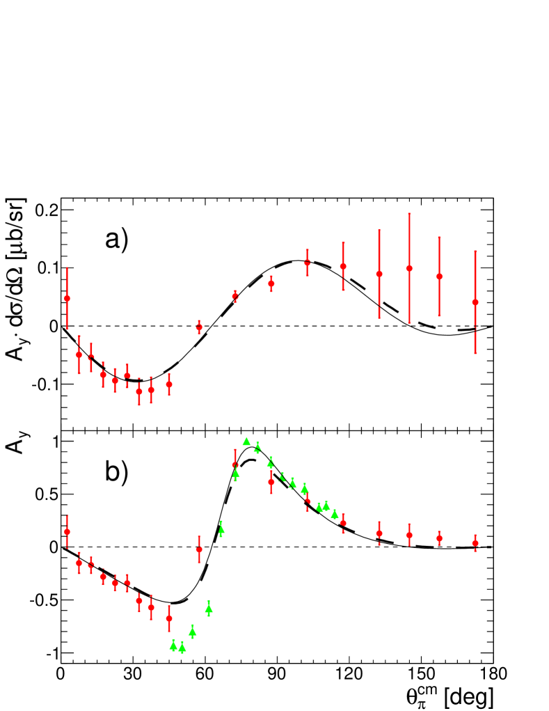
Figure 4: (a) The product of the measured analysing power and differential cross section for the $\pol{p}n\to\{pp\}_{s}\pi^{-}$ reaction at 353 MeV, where the error bars shown are statistical and do not include the 11% systematic uncertainty. The dashed curve represents the best fit of Eq. (2) with $b_{1}$, $b_{2}$, and $b_{3}$ terms whereas the solid one corresponds to the global fit to all the data. (b) Measured values of $A_{y}$ for the $\pol{p}n\to\{pp\}_{s}\pi^{-}$ reaction showing both the ANKE (circles) and TRIUMF data [5] (triangles). The systematic uncertainty in the ANKE data is 9%. The lines represent the quotients of the fits in panel-a and those to the cross section in Fig 3.

Fitting the weighted $A_{y}$ distribution with the form of Eq. (2) requires at least the three terms given in Table 1. The associated curve is shown in Fig. 4a and this divided by the parameterisation of the cross section in panel b.

The spin structure of the $pn\to\{pp\}_{s}\pi^{-}$ reaction is identical to that of $pp\to\{pp\}_{\!s\,}\pi^{0}$, which was already presented in [3]. The cross section and analysing power can be written in terms of two scalar amplitudes $A$ and $B$ through

$$\left(\frac{d\sigma}{d\Omega}\right)_{\!0} = \frac{k}{4p}\left(|A|^{2}+|B|^{2}+2\,\textrm{Re}[AB^{*}]\cos\theta_{\pi}\right)\!,$$

$$A_{y}\left(\frac{d\sigma}{d\Omega}\right)_{\!0} = \frac{k}{4p}\left(2\,\textrm{Im}[AB^{*}]\sin\theta_{\pi}\right)\!.$$ (3)

Keeping terms up to pion $d$ waves, the $pp\to\{pp\}_{\!s\,}\pi^{0}$ data at 353 MeV [3] can be parameterised in terms of the three amplitudes $M_{s}^{P}$, $M_{d}^{P}$, and $M_{d}^{F}$, corresponding to the transitions, ${}^{3\!}P_{0}\to\,^{1\!}S_{0}s$, ${}^{3\!}P_{2}\to\,^{1\!}S_{0}d$, and ${}^{3\!}F_{2}\to\,^{1\!}S_{0}d$, respectively. In proton-neutron collisions there are also the two $p$-wave transitions, ${}^{3\!}S_{1}\to\,^{1\!}S_{0}p$ and ${}^{3\!}D_{1}\to\,^{1\!}S_{0}p$ that arise in the isospin $I=0$ case, and for these we introduce amplitudes $M_{p}^{S}$ and $M_{p}^{D}$, respectively.

In terms of these partial waves, $A$ and $B$ become

$$A = \frac{1}{\sqrt{2}}\left[M_{s}^{P}-\mbox{${\textstyle\frac{1}{3}}$}M_{d}^{P}+M_{d}^{F}\left(\cos^{2}\theta_{\pi}-\mbox{${\textstyle\frac{1}{5}}$}\right)+M_{p}^{D}\cos\theta_{\pi}\right],$$

$$B = \frac{1}{\sqrt{2}}\left[M_{p}^{S}-\mbox{${\textstyle\frac{1}{3}}$}M_{p}^{D}+\left(M_{d}^{P}-\mbox{${\textstyle\frac{2}{5}}$}M_{d}^{F}\right)\cos\theta_{\pi}\right].$$ (4)

It is clear from the very different behaviour of the angular distributions for $\pi^{0}$ and $\pi^{-}$ production that the extra $p$-wave amplitudes in Eq. (4) must be very large and that it will not be justified to discard their interference with $M_{d}^{P}$.

Keeping terms up to $p$–$d$ interference but omitting the squares of the $d$-wave amplitudes, we find that

$$a_{0} = \mbox{${\textstyle\frac{1}{2}}$}|{M}^{P}_{\rm s}|^{2}+\mbox{${\textstyle\frac{1}{2}}$}|{M}^{S}_{\rm p}-\mbox{${\textstyle\frac{1}{3}}$}{M}^{D}_{\rm p}|^{2}-\mbox{${\textstyle\frac{1}{3}}$}\mathrm{Re}\left[{M}^{P*}_{\rm s}({M}^{P}_{\rm d}+\mbox{${\textstyle\frac{3}{5}}$}{M}^{F}_{\rm d})\right]$$

$$a_{1} = \mathrm{Re}\left[{M}^{P*}_{\rm s}({M}^{S}_{\rm p}+\mbox{${\textstyle\frac{1}{3}}$}{M}^{D}_{\rm p})+\mbox{${\textstyle\frac{2}{3}}$}{M}^{P*}_{\rm d}({M}^{S}_{\rm p}-\mbox{${\textstyle\frac{5}{6}}$}{M}^{D}_{\rm p})\right.$$

$$\left.-\mbox{${\textstyle\frac{3}{5}}$}{M}^{F*}_{\rm d}{M}^{S}_{\rm p}\right]$$

$$a_{2} = \mbox{${\textstyle\frac{1}{6}}$}|{M}^{D}_{\rm p}|^{2}+\mathrm{Re}\left[{M}^{P*}_{\rm s}({M}^{P}_{\rm d}+\mbox{${\textstyle\frac{3}{5}}$}{M}^{F}_{\rm d})+{M}^{S*}_{\rm p}{M}^{D}_{\rm p}\right]$$

$$a_{3} = \mathrm{Re}\left[[{M}^{D*}_{\rm p}({M}^{P}_{\rm d}+\mbox{${\textstyle\frac{4}{15}}$}{M}^{F}_{\rm d})+{M}^{S*}_{\rm p}{M}^{F}_{\rm d}\right]$$

$$b_{1} = \mathrm{Im}\left[({M}^{S*}_{\rm p}-\mbox{${\textstyle\frac{1}{3}}$}{M}^{D*}_{\rm p})({M}^{P}_{\rm s}-\mbox{${\textstyle\frac{1}{3}}$}({M}^{P}_{\rm d}+\mbox{${\textstyle\frac{3}{5}}$}{M}^{F}_{\rm d}))\right]$$

$$b_{2} = \mathrm{Im}\left[{M}^{S*}_{\rm p}{M}^{D}_{\rm p}-{M}^{P*}_{\rm s}({M}^{P}_{\rm d}-\mbox{${\textstyle\frac{2}{5}}$}{M}^{F}_{\rm d})\right]$$

$$b_{3} = \mathrm{Im}\left[{M}^{P*}_{\rm d}{M}^{D}_{\rm p}-{M}^{F*}_{\rm d}({M}^{S}_{\rm p}+\mbox{${\textstyle\frac{1}{15}}$}{M}^{D}_{\rm p})\right]\ .$$ (5)

By neglecting the small coupling between the ${}^{3\!}P_{2}$ and ${}^{3\!}F_{2}$ partial waves, and imposing the Watson theorem to determine the phases, it was possible to extract values for the complex amplitudes $M_{s}^{P}$, $M_{d}^{P}$, and $M_{d}^{F}$ from the analysis of the $pp\to\{pp\}_{\!s\,}\pi^{0}$ reaction [3]. Such an approach would not be valid for the two $p$-wave terms because of the very strong coupling between the incident ${}^{3\!}S_{1}$ and ${}^{3\!}D_{1}$ waves. Nevertheless, although there is a significant overall relative uncertainty between the $\pi^{-}$ and $\pi^{0}$ production data, associated with luminosity and other systematic effects, it is clear from the comparison of the seven free parameters in Eq. (5) with the ten observables in Table 1 that the system is over determined. As a consequence, if an acceptable solution is achieved it would support the approximation made in our analysis, such as the neglect of higher partial waves, $d$-$d$ interference and the effect of coupling between the ${}^{3\!}P_{2}$ and ${}^{3\!}F_{2}$ partial waves

The best fit to the combined $pp\to\{pp\}_{\!s\,}\pi^{0}$ and $pn\to\{pp\}_{s}\pi^{-}$ data sets is obtained with

$$M_{s}^{P} = \phantom{-}(55.3\pm 0.4)-(14.7\pm 0.1)i~{}\sqrt{\textrm{nb/sr}},$$

$$M_{d}^{P} = -(26.6\pm 1.1)-(8.6\pm 0.4)i~{}\sqrt{\textrm{nb/sr}},$$

$$M_{d}^{F} = \phantom{-(}5.3\pm 2.3~{}\sqrt{\textrm{nb/sr}},$$

$$M_{p}^{S} = -(32.4\pm 2.2)+(17.3\pm 2.7)i~{}\sqrt{\textrm{nb/sr}},$$

$$M_{p}^{D} = -(109.6\pm 9.6)+(140.7\pm 4.0)i~{}\sqrt{\textrm{nb/sr}}.$$ (6)

Since this solution has $\chi^{2}/\textrm{NDF}=89/82$, it shows that our truncated expansions can give a very good description of the data. The contribution from the ${}^{3\!}F_{2}\to\,^{1\!}S_{0}d$ transition is clearly very small and, if one eliminated $M_{d}^{F}$ completely, it would give only a marginally poorer fit with $\chi^{2}/\textrm{NDF}=94/82$. Note, whereas the phases of $M_{s}^{P}$, $M_{d}^{P}$ and $M_{d}^{F}$ were imposed (see above), the phases of $M_{p}^{S}$ and $M_{p}^{D}$ were extracted from the data.

The quality of the fits can also be judged from the comparison of the curves in Figs. 3 and 4 with the data. The residual small discrepancies in the description of the analysing power might, of course, be due to the neglect of some of the smaller terms. However, it should also be borne in mind that the main systematic uncertainty, namely the relative normalisations between the $pp\to\{pp\}_{\!s\,}\pi^{0}$ and $pn\to\{pp\}_{s}\pi^{-}$ data sets, has not been included in the determination of the parameters. On the other hand, adjusting this by a few percent would not lead to any qualitative changes in the solution of Eq. (6).

Another way of judging the changes introduced by making a global fit to all the data simultaneously rather than fits to individual distributions is to look by how much the parameters themselves were changed by this procedure. These are shown in Table 1. No changes at all are to be noticed for the $pp\to\{pp\}_{\!s\,}\pi^{0}$ reaction and for the $pn\to\{pp\}_{s}\pi^{-}$ case it is only $a_{3}(pn)$ where the difference is greater than the error bars.

The conclusions that one can draw from Eq. (6) are first that, although $d$-wave pion production is significant, this is almost exclusively from the ${}^{3\!}P_{2}$ state since the ${}^{3\!}F_{2}\to\,^{1\!}S_{0}d$ transition is very weak. In the $pn\to\{pp\}_{s}\pi^{-}$ case the amplitudes are dominated by the ${}^{3\!}D_{1}\to\,^{1\!}S_{0}p$ transition.

A partial wave decomposition of the TRIUMF $\pol{p}n\to\{pp\}_{s}\pi^{-}$ data was attempted [5] but at the time there were no $\pi^{0}$ production results available to constrain the fit and the authors had to rely on the application of the Watson theorem even for the ${}^{3\!}S_{1}$ and ${}^{3\!}D_{1}$ waves, which are strongly coupled. Furthermore, their data did not extend over the whole angular domain and so it is not surprising that their partial wave results bear little relation to ours. They found negligible $d$-wave production and did not identify the dominant role played by the ${}^{3\!}D_{1}\to\,^{1\!}S_{0}p$ transition.

In summary, we have measured the differential cross section and proton analysing power of $\pi^{-}$ production in the quasi-free $\pol{p}n\to\{pp\}_{s}\pi^{-}$ reaction in the 353 MeV energy region over the whole angular domain. These complement the analogous data obtained on $\pi^{0}$ production in the $\pol{p}p\to\{pp\}_{\!s\,}\pi^{0}$ reaction. Through a careful use of the Watson theorem, an amplitude analysis of the combined data sets has been achieved and these have allowed the determination of the partial waves up to $\ell_{\pi}=2$.

Some of the biggest uncertainties in the global amplitude analysis arise from the normalisations in the $pp\to\{pp\}_{\!s\,}\pi^{0}$ and $pn\to\{pp\}_{s}\pi^{-}$ data, which affect primarily the $s$- and $p$-wave production, respectively. The relative normalisation can be determined independently through a measurement of the transverse spin correlation parameter $A_{x,x}$ for the $pn\to\{pp\}_{s}\pi^{-}$ reaction [21]. Such data have already been taken and, when the results are available in 2012, these will make the amplitude analysis more robust.

The pion-production amplitudes extracted must now be analysed using chiral perturbation theory and this will be an important step to provide a deeper understanding of low energy pion dynamics. If this programme is successful, it will provide further strong evidence that chiral perturbation theory can indeed be applied to $NN\to NN\pi$ provided that the large momentum transfers are taken into account properly. This is a precondition for the analysis of isospin-violating reactions in the same framework [22, 23, 24], which will shed light on the role of the quark mass term in low energy pion reactions.

We are grateful to other members of the ANKE Collaboration for their help with this experiment and to the COSY crew for providing such good working conditions, especially of the polarised beam. This work has been partially supported by the BMBF (grant ANKE COSY-JINR), RFBR (09-02-91332), DFG (436 RUS 113/965/0-1), the JCHP FFE, the SRNSF (09-1024-4-200), the Helmholtz Association (VH-VI-231), STFC (ST/F012047/1 and ST/J000159/1), and the EU Hadron Physics 2 project “Study of strongly interacting matter”

References

- [1] A. Kacharava, F. Rathmann, and C. Wilkin, Spin Physics from COSY to FAIR, COSY proposal 152 (2005), arXiv:nucl-ex/0511028.
- [2] C. Hanhart, Phys. Rept. 397 (2004) 155.
- [3] D. Tsirkov et al., submitted for publication.
- [4] F. Duncan et al., Phys. Rev. Lett. 80 (1998) 4390.
- [5] H. Hahn et al., Phys. Rev. Lett. 82 (1999) 2258.
- [6] S. Barsov et al., Nucl. Instrum. Methods A 462 (1997) 364.
- [7] A. Khoukaz et al., Eur. Phys. J. D 5 (1999) 275.
- [8] R. Schleichert et al., IEEE Trans. Nucl. Sci. 50 (2003) 301.
- [9] A. Mussgiller, Ph.D. thesis, Hamburg, (2005).
- [10] G. Riepe et al., Nucl. Instrum. Methods A 177 (1980) 361.
- [11] S. Dymov et al., Phys. Rev. C 81 (2010) 044001.
- [12] S. Agostinelli et al., Nucl. Instrum. Methods A 506 (2003) 250.
- [13] I. Fröhlich et al., Proc. XI Int. Workshop Advanced Computing and Analysis Techniques in Physics Research, PoS(ACAT)(2007) 076; arXiv:0708.2382 [nucl-ex].
- [14] K. M. Watson, Phys. Rev. 88 (1952) 1163; A. B. Migdal, Sov. Phys. JETP 1 (1955) 2.
- [15] S. Dymov et al., Phys. Lett. B 635 (2006) 270.
-
[16]
R. A. Arndt et al., Phys. Rev. C
76 (2007) 025209;
http://gwdac.phys.gwu.edu. - [17] R. Machleidt, K. Holinde, and Ch. Elster, Phys. Rep. 149 (1987) 1.
- [18] H. Hahn et al., Phys. Rev. C, 53 (1996) 1074.
- [19] V. Baru et al., Phys. Rev. C 80 (2009) 044003.
- [20] R. Bilger et al., Nucl. Phys. A 663 (2001) 633.
- [21] S. Dymov et al., COSY proposal #205 (2010).
- [22] A. Filin et al., Phys. Lett. B 681 (2009) 423.
- [23] A. Gardestig et al., Phys. Rev. C 69 (2004) 044606.
- [24] A. Nogga et al., Phys. Lett. B 639 (2006) 465.