One dimensional Fokker-Planck reduced dynamics of decision making models in Computational Neuroscience

Abstract

We study a Fokker-Planck equation modelling the firing rates of two interacting populations of neurons. This model arises in computational neuroscience when considering, for example, bistable visual perception problems and is based on a stochastic Wilson-Cowan system of differential equations. In a previous work, the slow-fast behavior of the solution of the Fokker-Planck equation has been highlighted. Our aim is to demonstrate that the complexity of the model can be drastically reduced using this slow-fast structure. In fact, we can derive a one-dimensional Fokker-Planck equation that describes the evolution of the solution along the so-called slow manifold. This permits to have a direct efficient determination of the equilibrium state and its effective potential, and thus to investigate its dependencies with respect to various parameters of the model. It also allows to obtain information about the time escaping behavior. The results obtained for the reduced 1D equation are validated with those of the original 2D equation both for equilibrium and transient behavior.

1 Introduction

In this work, we will propose a procedure to reduce rate models for neuron dynamics to effective one dimensional Fokker-Planck equations. These simplified descriptions will be obtained using the structure of the underlying stochastic dynamical system. We will emphasize the numerical and practical performance of this procedure coming from ideas used in the probability community [5] for a particular model widely studied in the computational neuroscience literature.

We will consider a simple model [15, 13, 12] formed by two interacting families of neurons. We assume that there is a recurrent excitation with a higher correlation to the activity of those neurons of the same family than those of the other while a global inhibition on the whole ensemble is due to the background activity. These families of neurons are modelled through the dynamics of their firing rate equations as in the classical Wilson-Cowan equations [17]. The synaptic connection coefficients $w_{ij}$, representing the strength of the interaction between population $i$ and $j$, are the elements of a $2\times 2$ symmetric matrix $W$ given by

$$W=\left[\begin{array}[]{ccc}w_{+}-w_{I}&\phantom{t}&w_{-}-w_{I}\\ w_{-}-w_{I}&\phantom{t}&w_{+}-w_{I}\end{array}\right],$$

Here, $w_{+}$ is the self-excitation of each family, $w_{-}$ the excitation produced on the other family, and $w_{I}$ the strength of the global inhibition. The typical synaptic values considered in these works are such that $w_{-}<w_{I}<w_{+}$ leading to cross-inhibition since $w_{-}<w_{I}$ and self-excitation since $w_{I}<w_{+}$. Let us comment that these rate models are very simplified descriptions of interacting neuron pools, more accurate microscopic models introducing neuron descriptions at the level of voltage and/or conductances probability distribution can be derived [6, 7, 8, 9, 10, 11].

The time evolution for the firing rates $\nu_{i}(t)$ of the neuronal populations $i=1,2$ as given in [12] follows the following Stochastic Differential Equations (SDE):

$$\tau\frac{d\nu_{i}(t)}{dt}=-\nu_{i}(t)+\phi\left(\lambda_{i}+\sum_{j=1,2}w_{ij}\nu_{j}(t)\right)+\beta_{i}\xi_{i}(t),\quad i=1,2,$$ (1)

where $\tau=10^{-2}s$ is a time relaxation coefficient, which will be chosen equal to 1 in the sequel except for the numerical results, and $\xi_{i}(t)$ represents a white noise of normalized standard deviation $\beta_{i}>0$. In (1) the function $\phi(x)$ is a sigmoid function determining the response function of the neuron population to a mean excitation $x(t)=\lambda_{i}+\sum_{j}w_{ij}\nu_{j}$:

$$\phi(x)=\frac{\nu_{c}}{1+{\rm exp}(-\alpha(x/\nu_{c}-1))},$$

where $\lambda_{i}$ are the external stimuli applied to each neuron population.

We will recall in the next section that the study of the decision making process for the previous network can be alternatively studied by means of the evolution of a Fokker-Planck equation in two dimensions i.e. the plane $(\nu_{1},\nu_{2})$. The theoretical study of such problem (existence and uniqueness of positive solutions) was done in [3]. However, we will emphasize that due to slow-fast character of the underlying dynamical system the convergence towards the stationary state for the corresponding two-dimensional problem is very slow leading to a kind of metastable behavior for the transients.

Nevertheless, the 2D Fokker-Planck equation allows us to compute real transients of the network showing this metastable behavior. Moreover, we can derive a simplified one dimensional SDE in Section 3 by scaling conveniently the variables. Here, we use the spectral decomposition and the linearized slow manifold associated to some stable/unstable fixed point of the deterministic dynamical system. The obtained 1D Fokker-Planck equation leads to a simple problem to solve both theoretically for the stationary states and numerically for the transients. In this manner, we can reduce the dynamics on the slow manifold to the movement of a particle in an effective 1D potential with noise. We recover the slow-fast behavior in this 1D reduction but, due to dimension, we can efficiently compute its numerical solution for much larger times than the 2D. We can also directly compute an approximation to the 2D equilibrium state by the 1D equilibrium onto the slow manifold since in 1D, every drift derives from a potential.

Let us mention that another approach to get an approximation of the 2D Fokker-Planck equation by 1D Fokker-Planck reduced dynamics has been proposed in [16]. This approach is purely local via Taylor expansion around the bifurcation point leading to a cubic 1D effective potential. Moreover, an assumption about the scaling of the noise term is performed to be able to close the expansion around the bifurcation point. Our approach is valid no matter how far we are from the bifurcation point as long as the system has the slow-fast character and we do not assume any knowledge of the scaling of the noise term. Moreover, we can reconstruct the full potential not only locally at the bifurcation point. We point out that the results of their 1D Fokker-Planck reduction are compared to experimental data in [16] with excellent results near the bifurcation point. A similar applied analysis of our reduced Fokker-Planck dynamics in a system of interest in computational nuroscience is underway [4].

Section 4 is devoted to show comparisons between the 2D and the reduced 1D Fokker-Planck equations both for the stationary states and the transients. We demonstrate the power of this 1D reduction in the comparison between projected marginals on each firing rate variable and on the slow linearized manifold. Finally, section 5 is devoted to obtain information of the simulation in terms of escaping times from a decision state and performance in the decision taken.

2 The two dimensional model

We will illustrate all our results by numerical simulations performed with the physiological values introduced in [12]: $\alpha=4$ and $\nu_{c}=20Hz$, $\lambda_{1}=15Hz$ and $\lambda_{2}=\lambda_{1}+\Delta\lambda$, with $\Delta\lambda=0$ for the unbiased case and $\Delta\lambda=0.01,0.05,0.1$ for the biased case. The noise parameter is chosen as $\beta=0.1$, and the connection coefficients are given by $w_{+}=2.35$, $w_{I}=1.9$ and $w_{-}=1-r(w_{+}-1)/(1-r)$ with $r=0.3$.

It is well known [12] that the deterministic dynamical system associated with (1) is characterized by a supercritical pitchfork bifurcation in terms of the parameter $w_{+}$ from a single stable asymptotic state to a two stable and one unstable equilibrium points. We recall that the unstable point is usually called spontaneous state while the two asymptotically stable points are called decision states. The behavior of the bifurcation diagram for the deterministic dynamical system defining the equilibrium points in terms of the $w_{+}$ parameter and with respect to $\Delta\lambda$ is shown in Figure 1. Observe that in the nonsymmetric ($\Delta\lambda\neq 0$) bifurcations, the pair of stable/unstable equilibrium points detaches from the branch of stable points.

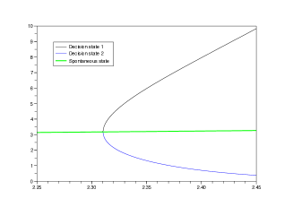
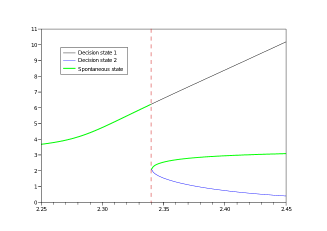
Figure 1: Bifurcation diagram: $\nu_{1}$-component of the equilibrium states with respect to $w_{+}$. Left Figure: bifurcation diagram for the unbiased case $\Delta\lambda=0$. Right Figure: bifurcation diagram for the biased case $\Delta\lambda=0.1$.

For example, with $w_{+}=2.35$ in the unbiased case, if $\Delta\lambda=0$, the stable points are in $S_{1}=(1.32,5.97)$ and its symmetric $S_{3}=(5.97,1.32)$, and the unstable one is in $S_{2}=(3.19,3.19)$; whereas, in the biased case $\Delta\lambda=0.1$ the stable points are in $S_{1}=(1.09,6.59)$ and $S_{3}=(5.57,1.53)$, and the unstable one in $S_{2}=(3.49,3.08)$.

Furthermore, it can be shown by means of direct simulations of system (1), that there is a slow-fast behaviour of the solutions toward the equilibrium points. This behavior is plotted in Figure 2, where the straight lines show the behavior of several realisations for the deterministic system (i.e. when $\beta_{i}=0$), and the wiggled line represent one realisation for the full stochastic system (1). Figure 2 highlights also the so called slow manifold: a curves in which the three equilibrium points of the system lie and where the dynamics are reduced to rather quickly.

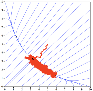
Figure 2: Dynamics of a firing rate towards stable equilibrium, fast convergence towards the slow manifold and slow convergence towards one of the stable equilibrium points along the slow manifold.

Applying standard methods of Ito calculus, see [14], we can prove that the probability density $p=p(t,\nu)$, with $t>0$ and $\nu=(\nu_{1},\nu_{2})$, satisfies a Fokker-Planck equation (known also as the progressive Kolmogorov equation). Hence, $p(t,\nu)$ must satisfy:

$$\partial_{t}p+\nabla\cdot\left((-\nu+\Phi(\Lambda+W\cdot\nu))p\right)-{{\beta^{2}\over 2}}\Delta p=0$$ (2)

where $\nu\in\Omega=[0,\nu_{m}]\times[0,\nu_{m}]$, $\Lambda=(\lambda_{1},\lambda_{2})$, $\Phi(x_{1},x_{2})=(\phi(x_{1}),\phi(x_{2}))$, $\nabla=(\partial_{\nu_{1}},\partial_{\nu_{2}})$ and $\Delta=\Delta_{\nu}$. We complete equation (2) by the following Robin boundary conditions or no flux conditions:

$$\left((-\nu+\Phi)p-{{\beta^{2}\over 2}}\nabla p\right)\cdot n=0$$ (3)

where $n$ is the outward unit normal to the domain.

Physically, this kind of boundary conditions means that we have no particles incoming in the domain. This is naturally relevant for the boundaries $[0,\nu_{m}]\times\{0\}$ and $\{0\}\times[0,\nu_{m}]$. For the two others boundaries, $[0,\nu_{m}]\times\{\nu_{m}\}$ and $\{\nu_{m}\}\times[0,\nu_{m}]$, it relies on the choice of $\nu_{m}$ large enough in such a way that the evolution of our system of particles is isolated. In practice, for the choosen parameters of our model, $\nu_{m}=10$ is a good choice.

In order to simplify notations, let us consider, from now on, the vector field $F=(F_{1},F_{2})$ representing the flux in the Fokker-Planck equation:

$$F(\nu)\stackrel{{\scriptstyle def}}{{=}}-\nu+\Phi(\Lambda+W\cdot\nu)=\left(\begin{array}[]{c}-\nu_{1}+\varphi(\lambda_{1}+w_{11}\nu_{1}+w_{12}\nu_{2})\\ -\nu_{2}+\varphi(\lambda_{2}+w_{21}\nu_{1}+w_{22}\nu_{2})\end{array}\right)$$ (4)

then, equation (2) and boundary conditions (3) read:

$$\partial_{t}p+\nabla\cdot\left(F\,p-{\beta^{2}\over 2}\nabla p\right)=0$$ (5)

$$\left(F\,p-{\beta^{2}\over 2}\nabla p\right)\cdot n=0$$ (6)

We refer to [3] for numerical results and a detailed mathematical analysis of the Fokker-Planck model (5)-(6): proof of the existence, uniqueness, and positivity of the solution, and its exponential convergence towards the equilibrium, or stationary state. Let us just recall that the equilibrium state cannot be analytically given because the flux does not derive from a potential, i.e. it is not in gradient form.

Moreover, we remark that the slow-fast structure leads to stiff terms and thus, to small time steps and large computational time. In fact, the slow exponential decay to equilibrium makes impossible to wait for time evolving computations to reach the real equilibrium. Hence, it is difficult to numerically analyze the effect of the various parameters of the model on the equilibrium state, and then the importance of deriving a simplified model capable of explaining the main dynamics of the original one is justified. Nevertheless, one could find the equilibrium state directly by numerical methods to find eigenfunctions of elliptic equations. The discussed slow-fast behavior will serve us, in the sequel, to reduce the dynamics of the system to a one dimensional Fokker-Planck equation.

3 One dimensional reduction

In this section we present the one dimensional reduction of system (1). We shall treat first the deterministic part, see 3.1, then the stochastic terms, section 3.2, and finally we describe the one dimensional Fokker-Planck model, see 3.3.

3.1 Deterministic dynamical system

The slow-fast behavior can be characterized by considering the deterministic system of two ordinary differential equations, i.e. (1) with $\beta_{i}=0$. Regardless of the stability character of the fixed point $S_{2}=(\nu_{1}^{eq},\nu_{2}^{eq})$, the slow-fast behavior is characterized by a large condition number for the Jacobian of the linearized system at the equilibrium point $S_{2}$, i.e., a small ratio between the smallest and largest eigenvalue in amplitude.

More precisely, let us write the deterministic part of the dynamical system (1) as follows:

$$\dot{\nu}=F(\nu),$$ (7)

where $\nu$ is a vector and $F(\nu)=-\nu+\Phi(\Lambda+W\nu)$ is the flux, see (4), as described in section 2. Let us denote $\nu^{eq}$ the spontaneous equilibrium point, so that $F(\nu^{eq})=0$. By spontaneous state we mean the only equilibrium before the bifurcation point and the unique unstable equilibrium point after the subcritical pitchfork bifurcation. This equilibrium point $\nu^{eq}$ is then parameterized by the bifurcation parameter $w_{+}$ and it has a jump discontinuity at the bifurcation point for nonsymmetric cases $\Delta\lambda\neq 0$. Hence, by construction:

$$(\nu_{1}^{eq},\nu_{2}^{eq})=\Phi(\Lambda+W(\nu_{1}^{eq},\nu_{2}^{eq})).$$

For the system (1), the linearized Jacobian matrix is given by:

$$J_{F}(z_{1},z_{2})=\left(\begin{array}[]{cc}-1+w_{11}\varphi^{\prime}(z_{1})&w_{12}\varphi^{\prime}(z_{1})\\ w_{21}\varphi^{\prime}(z_{2})&-1+w_{22}\varphi^{\prime}(z_{2})\end{array}\right),$$

where we have denoted by $z_{i}$ the values $z_{i}\stackrel{{\scriptstyle def}}{{=}}\lambda_{i}+w_{i1}\nu_{1}+w_{i2}\nu_{2}$.

We recall that $\nu^{eq}$ is an hyperbolic fixed point (saddle point) after the bifurcation while before it is an asymptotically stable equilibrium. Hence the Jacobian $J_{F}(\nu^{eq})$ has two real eigenvalues $\mu_{1}$ and $\mu_{2}$ being both negative before the bifurcation and of opposite signs after. The bifurcation is characterized by the point in which the smallest in magnitude eigenvalue becomes zero. Let us denote by $\mu_{1}$ the (large) negative eigenvalue and by $\mu_{2}$ the (small) negative/positive eigenvalue of $J_{F}(\nu^{eq})$. We remark that, the small parameter $\varepsilon<<1$ which is responsible for the slow-fast behavior is determined by the ratio of the amplitude of the two eigenvalues:

$$\varepsilon=\left|\frac{\mu_{2}}{\mu_{1}}\right|\,.$$ (8)

The values in terms of $w_{+}$ and for different values of $\Delta\lambda$ are shown in figure 3. In the range of parameters we are interested with, $\varepsilon$ is of the order of $10^{-2}$. Note the jump discontinuities at the bifurcation point for $\Delta\lambda\neq 0$ since the point around which our analysis can be performed jumps to the new created branch of the bifurcation diagram at the bifurcation point.

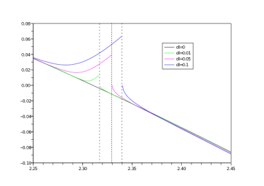
Figure 3: Eigenvalues ratio with respect to $w_{+}$ and for $\Delta\lambda=0,0.01,0.05,0.1$.

In order to reduce the system we need to introduce a new phase space based on the linearization of the problem. We will denote by $P$ the matrix containing the normalized eigenvectors and by $P^{-1}$ its inverse matrix. Note that, in the unbiased case ($\Delta\lambda=0$), we have:

$$P={1\over\sqrt{2}}\left(\begin{array}[]{cc}1&-1\\ 1&1\end{array}\right).$$ (9)

with the associated eigenvalues $\mu_{1}=-1.55$ and $\mu_{2}=0.036$, and the eigenvectors are orthogonal. Orthogonality of the eigenvectors is no longer true for the nonsymmetric biased problem $\Delta\lambda\neq 0$. Furthermore, using Hartman-Grobman theorem [1, 2], we know that the solutions of the dynamical system are topologically conjugate with its linearization in the neighbourhood of an hyperbolic fixed point, which is valid in our case for all values of the bifurcation parameter except at the pitchfork bifurcation. Let us write it as follows:

$$J_{F}(\nu^{eq})=PDP^{-1},$$ (10)

where $P$ is the matrix of eigenvectors and $D$ is the associated diagonal matrix. We can describe the coordinates $\nu$ in the eigenvector basis and centered on the saddle point $\nu^{eq}$ as follows:

$$\nu=\nu^{eq}+PX,$$ (11)

which gives the definition for the new variable $X=(x,y)$, see also figure 4:

$$X=P^{-1}(\nu-\nu^{eq}).$$

Figure 4: Change of variable from the phase space $(\nu_{1},\nu_{2})$ to $(x,y)$.

We can conclude that system (7) reads in the $X$ phase space as:

$$\dot{X}=H(X)$$ (12)

where $H(X)$ is the two dimensional vector defined by :

$$H(X)=P^{-1}F(\nu^{eq}+PX).$$

We remark that by means of the chain rule, the Jacobian $J_{H}(X)$ is given by:

$$J_{H}(X)=P^{-1}J_{F}(\nu^{eq}+PX)P,$$

and using (10) and that $X(\nu^{eq})=0$, we obtain that $J_{H}(0)=D$, which is the diagonal matrix in the change of variables (10).

Let us now make explicit the system (12) in terms of its components $f(x,y)$ and $g(x,y)$:

$$\begin{cases}\dot{x}=f(x,y)\\ \dot{y}=g(x,y)\end{cases},$$

where considering the definition of the flux $F$ given by (4):

$$f(x,y)=-x-(P^{-1}\nu^{eq})_{1}+(P^{-1}\Phi(\Lambda+W(\nu^{eq}+PX)))_{1}$$ (13)

$$g(x,y)=-y-(P^{-1}\nu^{eq})_{2}+(P^{-1}\Phi(\Lambda+W(\nu^{eq}+PX)))_{2}$$

Now, we can choose a new time scale for the fast variable $\tau=\varepsilon t$, with $\varepsilon$ given by (8), in such a way that for large time $t\simeq\varepsilon^{-1}$ then the fast variable $\tau\simeq 1$ and the variations $\frac{dx}{d\tau}\simeq O(1)$. Then, the fast character of the variable $x$ is clarified, see similar arguments in [5], and the system reads as

$$\begin{cases}\varepsilon\displaystyle\frac{dx}{d\tau}=f(x,y)\\[11.38109pt] \displaystyle\frac{dy}{dt}=g(x,y)\end{cases}\,.$$

Our model reduction assumption consists in assuming that the curve defined by equation $f(x,y)=0$ is a good approximation when $\epsilon\ll 1$ to the slow manifold. This manifold coincides with the unstable manifold that joins the spontaneous point $\nu^{eq}$ to the two other stable equilibrium points ($S_{1}$ and $S_{3}$) after the bifurcation point while is part of the stable manifold before the pitchfork bifurcation.

Due to the non-linearity of the function $f$, see (13) and (4), we cannot expect an explicit formula for $f(x,y)=0$. Nevertheless, since $\partial_{x}f(0,0)\neq 0$, the resolution in the neighborhood of the origin is given by the implicit function theorem. Hence we can define a curve:

$$x=x^{*}(y)$$ (14)

such that $f(x^{*}(y),y)=0$ in a neighbourhood of the origin. We also note that, by construction the approximated slow manifold $x^{*}(y)$, implicitly defined by (14), intersects the exact slow manifold at all equilibrium points, i.e. where both $f$ and $g$ vanish (nullclines). Finally, we can conclude the slow-fast ansatz, replacing the complete dynamics by the one on the approximated slow manifold, and obtain the reduced one dimensional differential equation:

$$\dot{y}=g(x^{*}(y),y).$$

3.2 Stochastic term

We consider now the stochastic terms of system (1). When changing the variable form $\nu$ to $X$, also the standard deviation of the considered Brownian motion should be modified. Indeed the new variables $x$ and $y$ are linear combination of $\nu_{1}$ and $\nu_{2}$. For instance, consider two stochastic differential eqautions: $d\nu_{i}=\beta_{i}d\xi_{i},$ where $\xi_{i}$ are two independent normalized white noises and $\beta_{i}$ are the two standard deviations, and take a linear combination of $\nu_{1}$ and $\nu_{2}$ with real constant coefficients $a_{1},a_{2}$: $x=a_{1}\nu_{1}+a_{2}\nu_{2}$. Then $x$ must obey to the following stochastic differential equation:

$$dx=\sqrt{(a_{1}\beta_{1})^{2}+(a_{2}\beta_{2})^{2}}d\xi.$$

In our case, $X=P^{-1}(\nu-\nu^{eq})$, then we have:

$$y=(P^{-1})_{21}(\nu_{1}-\nu_{1}^{eq})+(P^{-1})_{22}(\nu_{2}-\nu_{2}^{eq})$$

or developing and considering $d\nu_{i}=\beta_{i}d\xi_{i}$,

$$dy=(P^{-1})_{21}\beta_{1}d\xi_{1}+(P^{-1})_{22}\beta_{2}d\xi_{2}$$

Since in our model $\beta_{1}=\beta_{2}=\beta$, and considering the above discussion, we can write for a white noise $d\xi$:

$$dy=\beta\sqrt{\left((P^{-1})_{21}\right)^{2}+\left((P^{-1})_{22}\right)^{2}}d\xi.$$

Finally, we conclude that the reduced one dimensional model reads:

$$\dot{y}=g(x^{*}(y),y)+\beta_{y}d\xi$$ (15)

with $\beta_{y}=\beta\sqrt{\left((P^{-1})_{21}\right)^{2}+\left((P^{-1})_{22}\right)^{2}}$. We note that in the unbiased case $\beta_{y}=\beta$, since $P$ is given by (9).

3.3 One dimensional Fokker-Planck model

We can now consider the Fokker-Planck (or progressive Kolmogorov) equation associated to the one dimensional stochatic differential equation (15). This gives the reduced dynamics on the approximated slow manifold $x=x^{*}(y)$. Let us remark that this reduced SDE is obtained except at the bifurcation point and therefore valid whenever the slow-fast decomposition is verified or in other words whenever $\epsilon$ is small.

Consider the probability distribution function $q(t,y)$, for $t\geq 0$ and $y\in[-y_{m},+y_{m}]$, then it must obey to the following one dimensional Fokker-Planck equation:

$$\partial_{t}q+\partial_{y}\left(g(x^{*}(y),y)q-{\beta_{y}^{2}\over 2}\partial_{y}q\right)=0$$ (16)

with no-flux boundary conditions on $y=\pm y_{m}$:

$$g(x^{*}(y),y)q-{\beta_{y}^{2}\over 2}\partial_{y}q=0\,.$$

Since equation (16) is one dimensional, it is always possible to find the effective potential $G(y)$ being the derivative of the flux term $g(x^{*}(y),y)$. In other words, we can always define the potential function:

$$G(y)=\int_{0}^{y}g(x^{*}(z),z)dz.$$

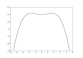
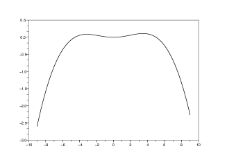
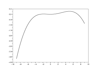
Figure 5: Comparison of the potential $-G$ for various values of $\Delta\lambda=0(top-left),0.01(top-right),0.05(bottom-left),0.1(bottom-right)$.

Moreover, we can explicitly obtain the stationary solutions of (16), i.e. the solutions $q_{s}(y)$ independent on time $t$, as follows:

$$q_{s}(y)=\frac{1}{Z}\exp(-2G(y)/\beta_{y}^{2})\,,$$ (17)

with $Z$ a suitable normalization constant. As explained also in [3], these stationary solutions are the asymptotic equilibrium states for the solution of the Fokker-Planck equation. In other words, letting time to go to infinity, the solution $q(t,y)$ to (16) must converge to $q_{s}(y)$. We have shown in [3] that the decay to equilibrium for the two dimensional problem was exponential. Nevertheless, this decay is so slow due to the small positive eigenvalue associated to the spontaneous state that the simulation shows metastable behavior for large times. Hence it is relevant to have a simple approximated computation of their asymptotic behavior without need to solve the whole 2D Fokker-Planck equation which is provided by this effective 1D potential.

4 1D model vs. 2D model

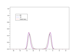
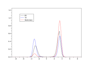
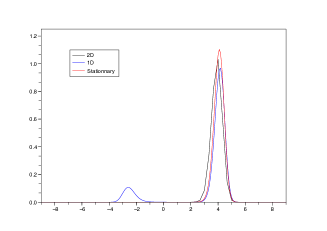
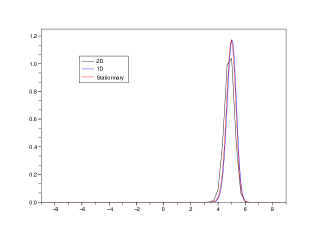
Figure 6: Comparison of the marginals in the new variable $y$, for differents values of the biasing paramter : $\Delta\lambda=0(top-left),0.01(top-right),0.05(bottom-left),0.1(bottom-right)$. Blue line: the marginal computed by means of the 1D problem. Black line: marginal computed from the 2D problem. Red line: the stationary marginal for the 1D. Final time is 400 seconds.

In this section, we numerically compare the solutions obtained for the one dimensional reduced Fokker-Planck equation (16) to the one of the original two dimensional model (5). Concerning the numerical scheme for the two dimensional problem, we refer the reader to the detailed description in [3]. In particular, we are interested in the solutions at equilibrium. As announced in section 3.3, we have an explicit formula for the solution at equilibrium in 1D (17) by computing the primitive $G(y)$. On the contrary, in the 2D setting, we cannot have such formulae and the computational time to approach equilibrium is very large.

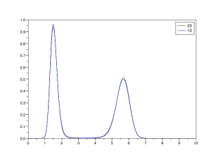
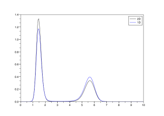
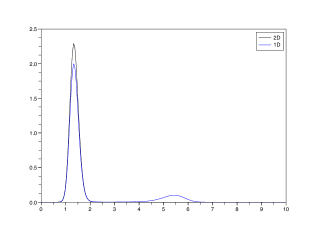
Figure 7: Comparison of the marginals in the variable $\nu_{1}$ for different values of the biasing parameter: $\Delta\lambda=0(top-left),0.01(top-right),0.05(bottom-left),0.1(bottom-right)$. Blue line: the marginal computed for the 1D problem at equilibrium. Black line: marginal computed from the 2D problem for time $T=400s$.

In Figure 6, we plot the solution at equilibrium of the 1D problem (the blue line) and compare it with the projection of the two dimensional solution on the new variable $y$ (the black line). We remark that the black line is not too smooth since we are projecting a 2D distribution on a uniform quadrangular mesh onto an inclined straight line. We can see a good matching in the unbiased case ($\Delta\lambda=0$). In the biased cases, the results are different: for $\Delta\lambda=0.01$, one clearly sees that even if we have computed until the final time of $400$ seconds, both the 2D and the 1D solutions have not reached equilibrium and the 2D results are closer to equilibrium; while for $\Delta\lambda=0.05,$ or $0.1$, the difference is smaller since the drift is strong enough to push all particles toward only one of the equilibrium points and there is only one population bump at least for the 2D results. The 2D results are closer to equilibrium at $\Delta\lambda=0.05$ while at $\Delta\lambda=0.1$ the 1D are closer.

On the other way round, we can also compare the marginals obtained from the two dimensional problem with the projections of the solution for the one dimensional problem on the $\nu_{1}$ and/or $\nu_{2}$ axes. In figure 7 we show the comparison for various $\Delta\lambda$. Note that $\Delta\lambda=0.01$ is the most interesting case as discussed in the previous figure. In fact, for larger $\Delta\lambda$, at equilibrium, the particles are almost all concentrated around one of the two stable points. Thus, no bump is visible around the second one (even in the one dimensional reduced solution), and for the unbiased case the matching is excellent. We warn the reader in order to compare Figures 6 and 7 that increasing values of $y$ correspond to decreasing values of $\nu_{1}$.

The results demonstrate that the 1D reduction is worth to obtain information about the behavior at equilibrium. In the next section, we shall investigate the time dependent solution $q(y,t)$ of equation (16).

4.1 Time dependent solution

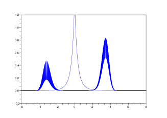
Figure 8: Evolution in time of the distribution in the $y$ variable, for the biasing parameter $\Delta\lambda=0.01$ with snapshot every dt= 20 or 0.2 s (left) and $20^{4}$ or 200s (right).

We are here interested also on the time behavior of the solution $q(y,t)$ of the 1D Fokker-Planck equation (16). For instance, we may compare the time evolution of momentum for the 2D and the reduced 1D problem. Thus, we need to compute not only the stationary solution of equation (16), but also its time dependent solution. We choose to discretize equation (16) using implicit in time finite difference method. The evolution of the 1D reduced model illustrates again the slow-fast character of this problem. In fact, we observe in Figure 8 the evolution in time of the density $q(y,t)$ for small (left) and for large (right) times respectively. The convergence toward the final stationary state is quite slow compared to the fast division toward the two bump distribution at the initial stages.

We describe now how to recover all the moments of the partial distribution function $p_{\varepsilon}$ in the $(\nu_{1},\nu_{2})$ plane, using the probability distribution function $q(y)$ solution of (16) and the approximated slow manifold $x^{*}(y)$.

The function $p_{\varepsilon}$ is concentrated along the the curve $\nu=(\nu_{1}(y),\nu_{2}(y))$ given by $\nu^{eq}+P(x^{*}(y),y)^{T}$, see (11). We parametrized this curve by means of a curvilinear coordinate and define

$$V(y)=\|P(x^{\prime*}(y),1)^{T}\|\,.$$

Then, for any test function $\Psi=\Psi(\nu_{1},\nu_{2})$, the moment $M_{\Psi}$ of the probability distribution function $p_{\varepsilon}=p_{\varepsilon}(\nu_{1},\nu_{2})$ is defined by

$$M_{\Psi}=\int_{\Omega}\Psi\,p_{\varepsilon}\,d\nu_{1}d\nu_{2}\,,$$

and given by

$$M_{\Psi}:=\int\Psi((\nu_{1}(y),\nu_{2}(y))q(y)dy\,.$$

This formulae can be used to compute either classical moments of $p_{\varepsilon}$ or marginals by choosing e.g. $\Psi=\delta_{\{\nu_{1}=\mu\}}$ to get the $\nu_{2}$-marginal as a function of $\mu$. Note that $q$ has to be normalized in such way that its total mass (along the slow manifold) is equal to $1$ i.e. $M_{\Psi\equiv 1}=1$.

Let us illustrate this metastability by the evolution of the first moments of the distribution in Figure 9. The initial data is a Dirac measure located above the spontaneous point ($x=0$, $y>0$ small). We choose $\Delta\lambda=0$, $\beta=0.3$ and $\omega_{+}=2.35$. We use a implicit scheme in order to have no stability constraint on the time step. The number of discretization point is 200 and the time step is $\Delta t=0.01$ for the left plot. It shows the fast dynamics: first the Dirac measure diffuses onto a Gaussian blob and moves quickly toward the spontaneous (unstable) state, then the Gaussian blob splits in the two bumps around the two stable equilibrium points. It seems that the solution has reached a equilibrium but it evolves very slowly. The figure on the right corresponds to $\Delta t=100$ and shows this slow evolution toward the real equilibrium state. We will comment more below.

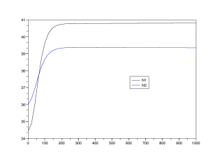
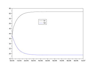
Figure 9: Evolution in time of the first order moments for the 1D Fokker-Planck reduction. Left Figure: final time is $10^{3}$. Right Figure: final time is $10^{7}$. Time unit is $0.01s$

We can finally compare the marginals in $\nu_{1}$ for the 1D reduced model and the 2D simulations in Figure 10. We can conclude that the transients of the 2D are captured extremely well by the 1D reduced model.

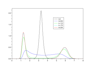
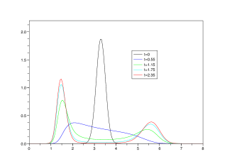
Figure 10: Comparison of the marginals in variable $\nu_{1}$, for the biasing parameter $\Delta\lambda=0.01$. Left Figure: 1D reduced model. Right Figure: 2D simulation.

5 Reaction time and Performance

In the previous sections, we have numerically studied the accuracy of the reduced 1D model with respect to the 2D original one. We discuss now some other information we can obtain from the 1D problem, namely: the escaping time, section 5.1, and the probability density to belong to a sub-domain of the phase space, section 5.2.

5.1 Escaping time

Fixed a bias $\Delta\lambda$ and for a variable $\beta$ we can easily compute the escaping time. In fact we recall that the Kramers formula [14]:

$$\mathbb{E}(t)\sim\exp(H_{G}/\beta^{2})$$

where $H_{G}$ is the maximum difference of the potential $G$

$$H_{G}=G_{max}-G_{min},$$ (18)

apply in the one dimensional framework, without needing to compute the solution $q(t,y)$ of the Fokker-Planck equation (16). Recall that $G_{max}$ corresponds to the potential value at the spontaneous state while $G_{min}$ corresponds to the minimum of the potential value at the two decision states. In Figure 11, we plot the potential gap computed by means of (18) as a function of the bias $\Delta\lambda$.

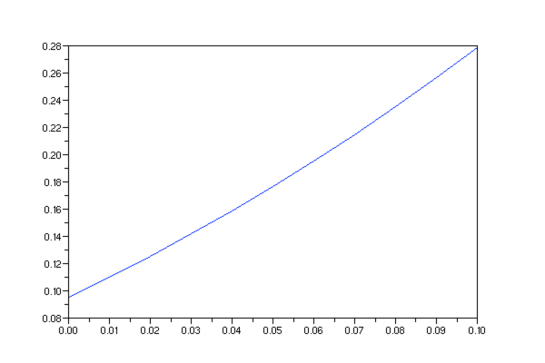
Figure 11: Computed potential gap as a function of $\Delta\lambda$.

In the 2D problem, since the drift is not the gradient of a potential, Kramer’s rule does not apply and the escaping times can only be computed for the unbiased case, $\Delta\lambda=0$. In fact, for $\Delta\lambda=0$ the problem is symmetric in $\nu_{1}$ and $\nu_{2}$ and thus, we know that the firing rates will separate in two identical bumps. Then, starting the computation from an initial data narrowly concentrated around one stable equilibrium point (say $S_{1}$), the escaping time $T$ can be defined as the time needed to have half of the total mass moving to a neighborhood of $S_{3}$. In particular, the expectation $\mathbb{E}(T)$ has an exponential behavior and its associated potential gap is $H_{G}=0.1$. Of course, this kind of argument cannot be extended to the biased case and thus, the 1D reduced model is essential.

5.2 Probability densities - Performance

We can compare the value of the probability $\rho_{i}$ of the firing rates to be in some domain $\Omega_{i}$ for the 2D Fokker-Plank model and the 1D reduced FP model. In particular, we shall compare: $\rho_{p}$ the probability for the 2D problem that at time $t$ the firing rates belong to $\{(x,y):y>0\}$; with $\rho_{+}$ representing the probability for the solution of the 1D problem to belong to $\Omega_{+}=[0,y_{m}]$, see Figure 4. We fix the standard derivation $\beta=0.1$, and let the bias $\Delta\lambda$ varying from $0$ to $0.05$, since the values of $\rho_{p}$ and $\rho_{+}$ for $\Delta\lambda$ bigger than $0.03$ are already very close (the relative error being of the order of $10^{-4}$).

We recall that, in the 2D problem, we has to wait for a very long time in order to reach equilibrium, since we have a meta-stable situation, see [3]. Nevertheless, we note that the $\rho_{p}(t)$ profile is exponentially increasing converging to an asymptotic value $\rho_{\infty}$. We can extrapolate this value from the values of $\rho_{p}(t)$ for some initial iterations as follows. Assume that the probability $\rho_{p}$ behaves like:

$$\rho(t)=\rho_{\infty}-a\exp(-t/\tau)$$

where $\rho_{\infty}$, $a$ and $\tau$ have to be determined by an “exponential regression”. For a sequence of time $t_{i}$ (of the form $t_{i}=t_{0}+T*i$, $i=0\cdots N$ that corresponds to the computed values of $\rho_{p}$), we define $\Delta\rho_{i}$ as the difference $\rho_{p}(t_{i})-\rho_{p}(t_{i}+T)$, we get:

$$\Delta\rho_{i}=a\exp(-t_{i}/\tau)(1-\exp(-T/\tau)).$$ (19)

Taking the $\log$ and the difference between two indexes $i$ and $j$ we obtain the expected value of $\tau$ as:

$$\tau\approx-{\log(\Delta\rho_{i})-\log(\Delta\rho_{j})\over t_{i}-t_{j}}.$$

Finally from (19), knowing $\tau$ (and $T$), we recover $a$, and the asymptotic limit $\rho_{\infty}$ is uniquely determined by:

$$\rho_{\infty}=\rho(t_{0})+a\exp(-t_{0}/\tau).$$ (20)

We show in Figure 12 the comparison between the values for the one dimensional computation (red line) and the one extrapolated from the 2D computation, see equation (20), using a final time of 20 seconds (blue line). Note that the non-smoothness of the blue line (2D extrapolation) may be due to the fact that for computing $\rho_{p}$ we need to compute the inner product for any point $\nu$ of the phase space $(\nu_{1},\nu_{2})$ : $<(\nu_{eq}-\nu),P_{1,j}>$, and we choose for different values of $\Delta\lambda$ the same equilibrium point $\nu_{eq}$ and matrix $P$: for instance, for $\Delta\lambda=0.016,0.018,0.020,0.022,0.024$ we choose the values of $\Delta\lambda=0.020$:

$$\nu_{eq}=\left(\begin{array}[]{c}3.0448158\\ 3.2397474\end{array}\right)\;,\qquad P=\left(\begin{array}[]{cc}0.7003255&-0.6959201\\ 0.7138236&0.7181192\end{array}\right).$$

Figure 12: Comparison of the values for $\rho_{+}$ and $\rho_{\infty}$ with respect to the biasing parameter $\Delta\lambda\in[0,0.05]$. Red line: the values computed from the 1D reduced problem. Blue line: the values extrapolated from the 2D problem.

Acknowledgments

J. A. Carrillo is partially supported by the projects MTM2011-27739-C04 from DGI-MICINN (Spain) and 2009-SGR-345 from AGAUR-Generalitat de Catalunya. S. Cordier and S. Mancini are partially supported by the ANR projects: MANDy, Mathematical Analysis of Neuronal Dynamics, ANR-09-BLAN-0008-01. All authors acknowledge partial support of CBDif-Fr, Collective behaviour $\&$ diffusion : mathematical models and simulations, ANR-08-BLAN-0333-01.

References

- [1] Hartman, P. (1960) A lemma in the theory of structural stability of differential equations. Proc. A.M.S. 11 (4): 610?620. doi:10.2307/2034720.
- [2] Grobman, D.M. (1959) Homeomorphisms of systems of differential equations. Dokl. Akad. Nauk SSSR 128: 880-881.
- [3] Carrillo J. A., Cordier S., Mancini S. (2011) A decision-making Fokker-Planck model in computational neuroscience, J. Math. Biol. 63: 801-830.
- [4] Carrillo J. A., Cordier S., Deco G., Mancini S. (2011) General One-Dimensional Fokker-Planck Reduction of Rate-equations models for two-choice decision making. In progress.
- [5] Berglund N, Gentz B (2005) Noise-Induced Phenomena in Slow-Fast Dynamical Systems. A Sample-Paths Approach. Springer, Probability and its Applications
- [6] Brunel, N. (2000) Dynamics of sparsely connected networks of excitatory and inhibitory spiking networks. J. Comp. Neurosci., 8:183–208.
- [7] Brunel N., Hakim, V. (1999) Fast global oscillations in networks of integrate-and-fire neurons with long fiting rates. Neural Computation, 11:1621–1671.
- [8] Brunel, N., Wang X.-J. (2003) What determines the frequency of fast network oscillations with irregular neural discharge? I. synaptic dynamics and excitation-inhibition balance. J. Neurophysioly, 90:415–430.
- [9] Cai D., Tao L., McLaughlin D. W. (2004) An embedded network approach for scale-up of fluctuation-driven systems with preservation of spike information. PNAS, 101:14288–14293.
- [10] Cai D., Tao L., Rangan A.V., McLaughlin D. W. (2006) Kinetic theory for neuronal network dynamics. Commun. Math. Sci., 4(1):97–127.
- [11] Cai D., Tao L., Shelley M. J., McLaughlin D. W. (2004) An effective kinetic representation of fluctuation-driven neuronal networks with application to simple and complex cells in visual cortex. PNAS, 101:7757–7762.
- [12] Deco G, Martí D (2007) Deterministic Analysis of Stochastic Bifurcations in Multi-stable Neurodynamical Systems. Biol Cybern 96(5):487-496.
- [13] La Camera G, Rauch A, Luescher H, Senn W, Fusi S (2004) Minimal models of adapted neuronal response to In Vivo-Like input currents. Neural Computation, 16(10):2101-2124.
- [14] Gardiner CW (1985) Handbook of Stochastic Methods for Physics, Chemistry and the Natural Sciences. Springer
- [15] Renart A, Brunel N, Wang X (2003) Computational Neuroscience: A Comprehensive Approach. Chapman and Hall, Boca Raton.
- [16] Roxin A, Ledberg A (2008) Neurobiological models of two-choice decision making can be reduced to a one-dimensional nonlinear diffusion equation. PLoS Computational Biology 4: 43–100.
- [17] Wilson HR, Cowan JD (1972) Excitatory and inhibitory interactions in localized populations of model neurons. Biophy. J., Vol. 12(1):1-24.