Approximating Constraint Propagation in Datalog

Abstract

We present a technique exploiting Datalog with aggregates to improve the performance of programs with arithmetic (in)equalities. Our approach employs a source-to-source program transformation which approximates the propagation technique from Constraint Programming. The experimental evaluation of the approach shows good run time speed-ups on a range of non-recursive as well as recursive programs. Furthermore, our technique improves upon the previously reported in the literature constraint magic set transformation approach.

1 Introduction

Datalog [15, 1] is a syntactic subset of Prolog introduced in the 1980s for database processing. By supporting a limited, safe form of recursion, Datalog considerably extends the expressive power of traditional database query languages like SQL. At the same time, unlike Prolog, Datalog allows SQL’s set-at-a-time evaluation. Also similarly to SQL, the programs in Datalog are guaranteed to terminate. Hence, extra-logical constructs such as Prolog’s cut (‘!’) operator are not needed.

After its original introduction as a smarter version of SQL, Datalog lost the interest of researchers for a time, until recently re-gaining attention in applications falling outside of the realm of traditional database reasoning, which include: program analysis [9, 8, 7], networks [13, 14], security protocols [11], knowledge representation [10], robotics [2] and gaming [20]. Our industrial partner, LogicBlox Inc. [12], uses a variant of Datalog, called Datalog^LB, as the basis for implementing decision automation and business planning systems.

Many of the above application domains rely on processing numerical data with arithmetic operations, in Datalog available as built-in relations (predicates). We focus in particular on built-in arithmetic (in)equality predicates ($>$, $<$, etc.) which we also refer to as (arithmetic) constraints. The existing Datalog compilers do not exploit the constraining properties of the arithmetic predicates, but rather implement them as ordinary tests. As a result, evaluation of programs with arithmetic constraints follows the naive generate-and-test approach, where ordinary predicates act as generators, and the entire search space that they produce is enumerated before the constraints can be applied to prune the candidate solutions. The research area of Constraint Programming (CP) offers approaches that prune the search space more eagerly, e.g., constrain-and-generate, as well as the constraint implementation technique, called constraint propagators, which allows to prune the domains of the variables involved in the constraints to narrow down the sets of candidate values even before the values are enumerated.

We adapt the CP constraint propagator technique to filter the individual generators in Datalog programs before they are used in the joins represented as arithmetic constraints. For this purpose we have developed an automatic program transformation framework in the Datalog^LB system. Experimental evaluation shows that our technique enables good run-time improvements for a variety of test programs.

2 Datalog^LB

LogicBlox is a commercial Datalog-based platform for building enterprise-scale corporate planning and pricing applications. LogicBlox is currently used in several commercial decision automation applications, including retail supply-chain management [16] and software program analysis [3, 4, 18]. A typical LogicBlox application involves computational analyses that require aggregation across very large data sets combined with simulation and modeling techniques. The platform accommodates these features by means of its custom query language Datalog^LB, a type-safe variant of Datalog, based on incremental evaluation, with trigger-like functionality and support for dynamic updates, declarative specification of functional dependencies, non-deterministic choice, stratified negation, meta-programming, and a wide range of extra-logical computations, including aggregation utilized by our optimization approach. In the following paragraphs we outline the main features of Datalog^LB and the LogicBlox run-time system. A more exhaustive description of Datalog^LB can be found in [22]. Readers familiar with Datalog may want to use this section as a reference when reading the remainder of the paper.

The Datalog^LB Language.

    1 digit(_) ->. 2 digit(d), val(d:v) -> uint[8](v), v<=9. 3  4 solution(i,a,m,s) -> digit(i), digit(a), digit(m), digit(s). 5 solution(i,a,m,s) <- 6    digit(i), val(i:vi), 7    digit(a), val(a:va), 8    digit(m), val(m:vm), 9    digit(s), val(s:vs), 10    vi != 0, 11    vs != 0, 12    vi != va, vi != vm, vi != vs, 13    va != vm, va != vs, 14    vm != vs, 15    vi*(10*va+vm) = 100*vs+10*va+vm.     

Figure 1: The Datalog^LB encoding of the I*AM=SAM cryptarithmetic puzzle.

Figure 1 shows a Datalog^LB encoding of the cryptarithmetic puzzle I*AM=SAM, the goal of which is to find the assignment of digits to letters that satisfies the equation I*AM = SAM.

The basic programming construct in Datalog^LB is the implication ‘<-’, denoting derivation rules of the form:

Head <- Body.where Head and Body are conjunctions of atoms. An atom can be either a predicate with variable or constant arguments, a comparison expression, an arithmetic expressions, or a negated atom. The above rule means that the atoms constituting Head can be derived from the atoms constituting Body. The example program in Figure 1 contains only one rule (lines 5-15), which derives the facts of the predicate solution based on the facts of the predicates digit and val, and the constraints represented as comparisons and arithmetic expressions on their arguments.

Datalog^LB extends Datalog with the notion of an integrity constraint of the form:

Lhs -> Rhs.Informally, the above constraint means that if Lhs is true, then Rhs must also be true, where Lhs and Rhs are conjunctions of atoms. The difference between a constraint and a rule is that a rule derives data for the atoms in its head, whereas a constraint checks that for the existing data matching its left-hand side, the right-hand side holds. The integrity constraints constitute the basis of Datalog^LB’s static type system, which guarantees at compile-time that certain kinds of constraints always hold for all possible instantiations of a given schema. Our approach uses integrity constraints to declare filter types which allow to reduce the domains of predicates subjected to arithmetic constraints.

Datalog^LB types are represented as unary predicates. Custom types may be defined using entity predicates. For instance, in Figure 1, the constraint in line 1 declares the entity predicate digit. The constraint in line 4 is a type declaration for the predicate solution, which states that for every tuple solution(i,a,m,s), the arguments i, a, m, and s must be digit entities. An entity predicate $P$ may be associated with a reference mode predicate, which uniquely identifies each element in $P$ with a value of a primitive type, thus allowing to access the specific entity elements from user applications. For instance, line 2 of Figure 1 declares a reference mode predicate val, which associates each entity element d in digit with v, an 8-bit unsigned integer value no greater than 9, thus binding the digit type to represent single-digit integers. The syntactic form val(d:v) denotes the one-to-one functional relation between d and v, and is reserved for declaring reference mode predicates. The decision to express digits as entities is dictated by one of the mechanisms contributing to Datalog^LB’s termination guarantee, which restricts the use of primitive types as arguments to built-in predicates such as arithmetic operations.

The extra-logical operations supported by LogicBlox, including aggregation computations, are represented by special-syntax rules of the form:

result[x1,...,xn]=v <- Op<<v=Method>> Body.The head of the rule uses Datalog^LB’s shorthand notation for declaring functional dependencies: result[x1,...,xn]=v declares the predicate result to be a function from x1,...,xn to v. The notation also allows declaring singleton (constant) values: p[]=v declares the predicate p to be a singleton that contains only the value v. The value can be retrieved through p[]. The right-hand side of the above rule, in addition to the conjunction of atoms in Body, includes a directive which specifies the type of the operation to be performed (e.g., aggregation), and the particular method (e.g., finding the minimum value) to be used. For instance, in Section 3.1 we show the following rule which finds the lower bound for the val predicate:

lb_digit[]=n <- agg<<n=min(v)>> digit(d), val(d:v).Above, agg states that the rule computes an aggregation, and min names the specific operation to be applied to the values referenced by v.

The LogicBlox Run-time System.

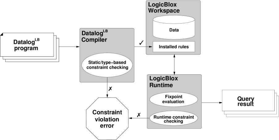
Figure 2: LogicBlox Architecture

Figure 2 illustrates the architecture of LogicBlox run time. After compilation, discussed in more detail in Section 4, the predicate definitions, rules, and constraints of the input Datalog^LB program are loaded into a designated data base instance called a workspace. The workspace may be then accessed (queried and/or modified) from the LogicBlox API. Whenever a user application adds or removes facts from a predicate, the LogicBlox run-time engine incrementally re-evaluates the installed program rules until the workspace reaches a fixed point, i.e., no more facts can be derived by the rules. At the same time the engine checks the program’s constraints, reporting any violations and restoring the workspace to a consistent state as needed.

3 The Filter Predicates Transformation

This section describes the details of our transformation, beginning with non-recursive programs, and then considering the impact of recursion.

3.1 Non-Recursive Programs

Recall the I*AM=SAM program from the previous section. Our goal is to reduce the number of different candidate values that are used for producing answers. Thus, we exploit the equality constraint

$$v_{i}*(10*v_{a}+v_{m})=100*v_{s}+10*v_{a}+v_{m}$$

from the program rule to filter candidate values in the generator predicate digit. Specifically, for each generator predicate atom appearing in the constraint, we consider the value generated by this atom in the context of the upper and lower bounds of the values produced by other generator atoms.

For instance, for the generator atom digit(i), the original constraint, which is equivalent to the pair of inequalities:

$$\left\{\begin{array}[]{l}v_{i}*(10*v_{a}+v_{m})\leq 100*v_{s}+10*v_{a}+v_{m}\\ v_{i}*(10*v_{a}+v_{m})\geq 100*v_{s}+10*v_{a}+v_{m}\end{array}\right.$$

yields the pair of inequalities:

$$\left\{\begin{array}[]{l}v_{i}*(10*\,l_{d}\,+\,l_{d}\,)\leq 100*u_{d}+10*u_{d}+u_{d}\\ v_{i}*(10*u_{d}+u_{d})\geq 100*\,l_{d}\,+10*\,l_{d}\,+\,l_{d}\end{array}\right.$$

where $u_{d}$ and $l_{d}$ represent the upper and lower bound of the generator predicate digit, respectively. We use these inequalities in the Datalog definition of the filter predicate for digit(i):

     digit_filtered_i(i) <-     digit(i),     val(i:vi),     lb_digit[]=t_1,     ub_digit[]=t_2,     vi* (10*t_1+t_1) <= 100*t_2+10*t_2+t_2,     100*t_1+10*t_1+t_1 <= vi* (10*t_2+t_2).     

Similar filter predicates are generated for the remaining generator atoms.

The bounds for the generator predicates are computed in separate aggregate predicates, and reused in all filter predicates:

     lb_digit[]=n <- agg<<n=min(v)>> digit(d), val(d:v).  ub_digit[]=n <- agg<<n=max(v)>> digit(d), val(d:v).     

In the last step of the transformation we replace the generator predicate atoms in the body of the solution/4 rule by atoms representing corresponding filter predicates:

     solution(i,a,m,s) <-     digit_filtered_i(i),     digit_filtered_a(a),     digit_filtered_m(m),     digit_filtered_s(s),     ... % rest of the original I AM SAM program     

Our approach is inspired by the well-known bounds consistency technique, in CP implemented by finite-domain constraint propagators. We simplify constraint propagation in two ways: (1) by computing filtered domains on the original domains rather than as a fixed point of the filtering process, and (2) by filtering only at the beginning of the evaluation rather than repeatedly after every enumeration step (in CP terminology known as labeling). As a consequence of these simplifications, (1) we cannot encode unbounded fixpoint computations, and (2) computing and storing many successively filtered tables for the same variable adds considerable time and space overhead. Nevertheless, our approach yields a light-weight technique that is easily provided on top of the existing Datalog implementations, offering a satisfactory compromise between the anticipated speed-up and the overhead.

3.2 Recursive Programs

     p(t,w) -> string(t), int[64](w).  s(t,w) -> string(t), int[64](w).    e(t,w) -> string(t), int[64](w).  e(t,w) <- p(t,w).  e(t,w) <- s(t,w),            e(tp,wp),            w - wp <= 100,            w + wp >= 19500.     

Figure 3: The Engine program.

Recursion considerably complicates our transformation. Consider the Engine program listed in Figure 3. The program selects suitable engines for an engine yard. In the predicates p(t,w), s(t,w) and e(t,w), t corresponds to the engine type and w to the produced wattage. The predicate p represents the primary engines, and the predicate s represents the potentially spare engines. A suitable engine for the engine compound e(t,w) is either a primary engine, or a spare engine that can assist another engine in the compound. The difference in wattage between the assisting engine and the assistee should not exceed 100, and the total wattage of the compound should be no less than 19,500.

         e(t,w) <- p(t,w).                         s_filtered(t,w) <-      e(t,w) <- s_filtered(t,w),                   s(t,w),                e_filtered(tp,wp),                 w-ub_e[] <= 100,                w-wp <= 100,                       19500 <= w+ub_e[].                w+wp >= 19500.                                                e_filtered(tp,wp) <-                                                   e(tp,wp),      lb_s[]=n <- agg<<n=min(v)>> s(_,v).          lb_s[]-wp <= 100,      ub_s[]=n <- agg<<n=max(v)>> s(_,v).          19500 <= ub_s[]+wp.      ub_e[]=n <- agg<<n=max(v)>> e(_,v). % ERROR     

Figure 4: Ill-formed Engine program after naive transformation.

The naive application of our technique yields the ill-formed program shown in Figure 4. The program involves recursion through aggregation: in order to compute the set of e/2 we need to know the upper bound of e/2. Such recursion is not supported by Datalog^LB (nor by any other LP system we are aware of).

Since it is not possible to effectively compute the exact upper bound on e/2, we approximate it as the upper bound of the approximated upper bounds of the two rules defining e/2. For the first, non-recursive rule, such an approximated (and exact) upper bound is ub_p[]. A crudely approximated upper bound for the second, recursive rule, is ub_s[]. Hence:

      ub_e[]=n <- n=max(ub_p[],ub_s[]).where

      ub_p[]=n <- agg<<n=max(v)>> p(_,v).

We may attempt to tighten the upper bound of the second rule, based on the observation that it is bounded from above by ub_e[]+100:

      ub_e[]=n <- n=max(ub_p[],min(ub_s[],ub_e[]+100)).Alas, this step reintroduces recursion through aggregation. We eliminate it in the same way as before, by substituting the cruder approximation derived earlier:

   ub_e[]=n <- n=max(ub_p[],min(ub_s[],max(ub_p[],ub_s[])+100).We further simplify the above expression by noticing that

$$\forall x,y,c\in\mathbb{N}.\min(x,\max(y,x)+c)=x$$

This step brings us back to the first approximation, thus proving that the refinement attempt was unsuccessful. Nevertheless, as we show in Section 5, our approximation is still quite effective at pruning the predicate domains and improving the performance of the programs.

4 Implementation

Most of the Datalog^LB syntax is compatible with the term syntax of standard Prolog. The discrepancies in the particular notations, such as the functional dependency syntax, can be easily accommodated by simple processing steps. Hence, we chose Prolog (specifically, SWI-Prolog [21]) to implement the transformations of Datalog^LB programs. Our analyzer consists of five Prolog modules, for the total of about 3,500 lines of Prolog code, including comments.

4.1 LogicBlox/SWI-Prolog Interface

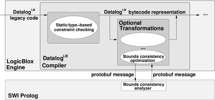
Figure 5: LogicBlox Compiler and its communication with SWI-Prolog

Figure 5 shows in more detail the LogicBlox compilation scheme and outlines the communication between the LogicBlox engine and the SWI-Prolog analyzer.

The LogicBlox compiler rewrites a source Datalog^LB program into a core representation, which is then encoded using Google’s protocol buffer (GPB) interface for further use by a number tools, including an interpreter. GPB [6] is a platform-independent, extensible mechanism for serializing structured data. GPBs allow the programmers to determine how to structure their data by defining simple data structures (messages) in a dedicated specification language, and then to compile those data structures into the language and platform of their choice. As shown in Figure 5, the core program representation generated by the LogicBlox compiler is either passed directly to the subsequent phase of run-time processing, or subjected to one or more optional transformations aimed at optimizing the compiled code or collecting information to be used in further evaluation steps. This infrastructure makes the GPBs the medium of choice for interfacing LogicBlox with external analysis modules. In case of our application, the entire interface, including simplified message specification (discussed below), comprises five new modules, for the total of 1,800 lines of code.

The interface on the SWI-Prolog side is based on the system’s native GPB library [17], which we extended with support for necessary features of Datalog^LB (e.g., recursively structured data), and optimized to linear run-time complexity. At this time our version of the library is available in a dedicated branch of the SWI-Prolog code repository.

The communication between LogicBlox and SWI-Prolog proceeds as follows. The output of the Datalog^LB compiler is received by a new LogicBlox module which extracts from it the information relevant to our analysis, encodes it as a collection of GPB messages, and opens a socket connection with SWI-Prolog. Once the connection is established, the messages are supplied to our analyzer. The analyzer decodes the messages into a program representation, applies the transformation, encodes the resulting program, and sends it back to the LogicBlox side, where another dedicated module retrieves the transformation results and updates the core representation of the program accordingly.

We illustrate the use of GPBs on Datalog^LB rule bodies. A rule body is a formula defined as an atom, a disjunction, a conjunction, or a negation. LogicBlox serializes and deserializes formulas with GBP messages of the following form:

         message Formula {          optional Atom atom = 1;          optional Negation negation = 2;          optional Conjunction conjunction = 3;          optional Disjunction disjunction = 4;      }      message Conjunction { repeated Formula formula = 1; }      ...      Note the mutually recursive nature of the Formula and Conjunction definitions.

On the SWI-Prolog side, the messages are defined in message/2 clauses:

     protobufs:message(formula,Template) :-      Template = [ optional(embedded(1,message(atom,_)),_)                 , optional(embedded(2,message(negation,_)),_)                 , optional(embedded(3,message(conjunction,_)),_)                 , optional(embedded(4,message(disjunction,_)),_)                 ].    protobufs:message(conjunction,Template) :-     Template = [ repeated(1,embedded(_,message(formula,_))) ].      The predicate message/2, which we added to the SWI-Prolog GPB library, enables naming message templates. It is essential for recursive and repeated embedded messages. The protobuf_message/2 predicate serializes and deserializes messages to and from binary form, like the representation of the single-atom formula digit(d).

     ?- protobuf_message(message(formula,          [ optional(embedded(1,                       message(atom,                           [ string(1,"digit"),                             repeated(2,embedded([ ...                                                   % Term for variable d                                                 ],term))                           ])),present),            optional(embedded(2,message(negation,_)),not_present),            optional(embedded(3,message(conjunction,_)),not_present),            optional(embedded(4,message(disjunction,_)),not_present)          ]),Bytes).     

4.2 The Transformation

Given a representation of a Datalog^LB program, our transformation processes in turn each of its rules. For every rule with one or more arithmetic constraints, it identifies the generator predicate atoms, exploits the constraints to produce corresponding filter predicates, and replaces the generator atoms accordingly. It also extends the program with the definitions for the auxiliary predicates performing bounds computations.

Implementation of the code that generates the bounds-computing predicates turned out to be one of the more involved aspects of our project. The numerical data appearing in the arithmetic constraints pertinent to our transformation is often represented as the values of the Datalog^LB reference mode predicates where the keys are the entities produced by the predicates serving as generators. To access these data, it is necessary to reconstruct the chain of functional dependencies connecting each value with the appropriate entity generator. For instance, to compute predicate bounds for the atom set:

p(x), val_1(x:vx), q(y), val_2(y:vy), vx > vywe need to reconstruct the chain connecting vx with p and vy with q. Additional complications arise when the reference mode predicates (and the corresponding generators) have non-unary keys, in which case the reconstructed dependencies are trees with the functional dependencies as nodes and the generators as leaves.

As mentioned in Section 2, Datalog^LB’s static type system relies on the type information in the form of the integrity constraints. To ensure completeness of the type information in the transformed programs, we need to provide type declarations for the predicates generated by the analyzer (i.e., filter and aggregate predicates). It turns out that we can conveniently derive these directly from the original predicates, with no additional bookkeeping during the transformation.

5 Evaluation

We now present the results of applying our transformation to a variety of programs. All experiments were performed using LogicBlox 3.7, on a machine with a 2.83 GHz Intel® Core™ 2 Quad CPU and 4 GB of RAM, running Ubuntu 10.10 (Linux kernel 2.6.35-24-server). Additionally, we report the results obtained by the tabled top-down evaluation using XSB Prolog 3.3.1. For each experiment we show run times, in seconds, for the original programs, and the relative performance change after the transformation.

The changes required to accommodate Datalog^LB programs in XSB are minimal and mainly syntactic in nature: we omitted type declarations, replaced ‘<-’ arrows with ‘:-’, modified variable names to begin with capital letters, changed functional dependencies to ordinary arguments, and provided implementation for aggregates. The key feature to guarantee termination is tabling: all predicates are declared tabled.

5.1 Non-Recursive Programs

Cryptarithmetic Puzzles.

Puzzle		DatalogLB		XSB
		Original	FP	Original	FP
I * AM =	SAM	$0.01$ sec.	$140.90$ %	$0.01$ sec.	$100.00$ %
BASE + BALL =	GAMES	$0.80$ sec.	$14.02$ %	$0.65$ sec.	$15.38$ %
SEND + MORE =	MONEY	$3.10$ sec.	$11.42$ %	$2.60$ sec.	$11.92$ %
BANJO + VIOLA =	VIOLIN	$2.67$ sec.	$12.79$ %	$2.73$ sec.	$12.09$ %
SATURN + URANUS =	PLANETS	$6.39$ sec.	$15.02$ %	$7.70$ sec.	$12.60$ %
SIX + SEVEN + SEVEN =	TWENTY	$3.90$ sec.	$27.05$ %	$8.75$ sec.	$25.26$ %
DONALD + GERALD =	ROBERT	$17.54$ sec.	$105.01$ %	$17.20$ sec.	$107.62$ %
BLACK + GREEN =	ORANGE	$20.63$ sec.	$11.71$ %	$19.99$ sec.	$52.53$ %

Table 1: Benchmark results for cryptarithmetic puzzles.

Table 1 reports the evaluation run times for a set of cryptarithmetic puzzles building on the idea of the I*AM=SAM program from Section 2. In almost all cases the transformation yields drastic performance improvements (3$\times$ to 10$\times$). There are two exceptions. In case of the I*AM=SAM benchmark, the overhead of the auxiliary predicates introduced by the transformation dominates the extremely short run time of the original program. In case of the DONALD+GERALD=ROBERT puzzle, the transformed program prunes very few values from the initial domains, and consequently shows performance similar to that of the original program.

The XSB evaluation yields similar results both in terms of the original program performance, and the benefits from the transformation.

The Production Problem.

The Production program models the mathematical programming problem of optimizing the profit from manufacturing several types of products, subject to a set of constraints such as production costs and maximum number of items to be manufactured for each product type, or the availability of the factory line. From the technical point of view this program is interesting because it contains multi-key functional dependencies that drive the filter predicates. Another non-standard feature is the use of the aggregates for computing the optimized profit.

Table 2 reports the results of evaluating the original and transformed program with four data sets differing in the range of the generator predicate indicating the number of tons of products being manufactured. Clearly, for LogicBlox evaluation, the transformation has no significant effect on the program for the small tons ranges, but enables a lot of pruning, and thus considerable performance improvement, when the tons ranges are large. On XSB the effects of the transformation are more uniform across the different data sets, with slightly better performance improvements for the larger tons ranges.

Tons range	DatalogLB		XSB
	Original	FP	Original	FP
[1,500]	$0.60$ sec.	$103.64$ %	$0.29$ sec.	$96.55$ %
[1,1000]	$2.81$ sec.	$100.75$ %	$1.10$ sec.	$98.18$ %
[1,2500]	$12.37$ sec.	$40.60$ %	$5.01$ sec.	$92.41$ %
[1,5000]	$13.71$ sec.	$41.27$ %	$5.90$ sec.	$88.30$ %

Table 2: Benchmark results for the Production problem.

5.2 Recursive programs

The Engine Program.

To evaluate the effects of our transformation on the recursive Engine program from Figure 3, we used four different data sets. Each data set defines the sets of couples produced by p/2 (denoted $P$ in the following), and s/2 (denoted $S$). Let

$$\mathcal{T}=\{{\rm Steam\;engine},{\rm Internal\;combustion\;engine},{\rm Gas\;Turbine}\}{\rm}$$

The four data sets define the sets $P$ and $S$ as follows.

• $Set_{1}$: $\left\{\begin{array}[]{rcl}P&=&\mathcal{T}\times[1100,11500]\\ S&=&\mathcal{T}\times[1,10000]\end{array}\right.$

• $Set_{2}$: $\left\{\begin{array}[]{rcl}P&=&\mathcal{T}\times[500,5000]\}\\ S&=&\mathcal{T}\times[1,6000]\}\end{array}\right.$

• $Set_{3}$: $\left\{\begin{array}[]{rcl}P&=&\mathcal{T}\times[500,16000]\}\\ S&=&\mathcal{T}\times[1000,14000]\}\end{array}\right.$

• $Set_{4}$: $\left\{\begin{array}[]{rcl}P&=&\mathcal{T}\times[10000,16000]\}\\ S&=&\mathcal{T}\times[8,12000]\}\end{array}\right.$

The results of the evaluation are shown in Table 3. There is a visible correlation between the particular data set and the effects of the transformation. With little pruning possible, we see a modest speed-up or even a slow-down, whereas considerable pruning yields large performance improvements.

Data set	DatalogLB		XSB
	Original	FP	Original	FP
$Set_{1}$	$26.87$ sec.	$21.41$ %	$43.40$ sec.	$6.11$ %
$Set_{2}$	$9.82$ sec.	$4.65$ %	$8.29$ sec.	$0.84$ %
$Set_{3}$	$172.47$ sec.	$84.18$ %	$119.82$ sec.	$64.91$ %
$Set_{4}$	$53.61$ sec.	$104.75$ %	$20.30$ sec.	$97.93$ %

Table 3: Benchmark results for the Engine program.

Multi-Legged Flights Program.

The Flights program (Figure 6) models multi-legged flights and their travel distance. More abstractly, it captures the transitive closure of a directed weighted graph. The Datalog^LB encoding consists of the basic variant of the program, based on that studied by Stuckey and Sudarshan [19], together with a sample query to compute all possible destinations no further than 10,000 miles from Sydney.

    1 e(x,y,d) -> string(x), string(y), int[64](d). 2  3 f(x,y,d) -> string(x), string(y), int[64](d). 4 f(x,y,d) <- e(x,y,d), d >= 0. 5 f(x,y,d) <- e(x,z,d1), d1 >= 0, 6             f(z,y,d2), d2 >= 0, 7             d = d1 + d2, d <= 10000. 8  9 query(x,y,d) -> string(x), string(y), int[64](d). 10 query("Sydney",y,d) <- f("Sydney",y,d), d >= 0, d <= 10000.     

Figure 6: The Datalog^LB encoding of the Flights program.

Predicate e(x,y,d) (line 1) denotes a flight leg, i.e., a direct connection between cities x and y with the distance d. The data of this predicate are given as facts. The predicate f (lines 3-7) defines a multi-legged flight as the transitive closure of the predicate e. Since the second rule for f contains recursion, to be expressible in Datalog^LB, it needs to be bounded. Hence, we have added the constraint ‘d <= 10000’ (line 7), which is not present in the encoding of [19]. Lines 9-10 define the query predicate.

It turns out that our transformation has no significant effect on the performance of the Flights program; it does not provide additional pruning. Fortunately, to our aid comes the constraint magic set transformation [19]. Not only is the constraint magic set rewritten (CMR) variant of the program (Figure 7) faster than the original, but also it is amenable to our transformation.

         answer_f(x,y,d) -> string(x), string(y), int[64](d).      answer_f(x,y,d) <-         x = "Sydney", f_a(x,y,d), d >= 0, d <= 10000.        f_a(x,y,d) -> string(x), string(y), int[64](d).      f_a(x,y,d) <-         query_f_a(x,ld,ud), ld <= ud,         e(x,y,d), d >= 0, d >= ld, d <= ud.      f_a(x,y,d) <-         query_f_a(x,ld,ud), ld <= ud,         e(x,z,d1), d1 >= 0,         f_a(z,y,d2), d2 >= 0,         d = d1 + d2, d >= ld, d <= ud.        query_f_a(x,ld,ud) -> string(x), int[64](ld), int[64](ud).      query_f_a("Sydney",0,10000).      query_f_a(y,ld2,ud2) <-         query_f_a(x,ld,ud), ld <= ud,         e(x,y,d), d >= 0,         ud2 = ud - d, ld2 = max(ld-d,0).            e(x,y,d) -> string(x), string(y), int[64](d).     

Figure 7: Constraint magic rewritten variant of the Flights program.

Table 4 shows the results of evaluating the CMR variant of the Flights program without (CMR) and with (CMR+FP) filter predicate transformation for a collection of 19 different data graphs. The graphs, generated using three different methods, have the following structure:

• there are six graphs with $n$ nodes, where each node has [0,$\lfloor n/m\rfloor$] random bi-directional edges with random distance in [0,10000].

• there are four graphs with $6\cdot n$ nodes consisting of 6 subgraphs with $n$ nodes. Within a subgraph, each node has $[0,m]$ bi-directional edges with distance [0,7000]. Each subgraph is connected to $[0,o]$ other subgraphs with distance [0,15000].

• there are nine graphs with $n\cdot m$ nodes, consisting of $m$ complete subgraphs of $n$ nodes that are not connected to one another.

For the LogicBlox evaluation, Table 4 reports performance decrease for three transformed programs with corresponding original run times below 0.1s, and visible improvement for all other benchmarks. The speed-up varies roughly between 2$\times$ for the original programs with the shorter run times and 8$\times$ for those with longer run times. Interestingly, the performance in XSB is very different. First, we observe that the run times for programs without the transformation are considerably shorter than in LogicBlox. Furthermore, applying the transformation has no effect on the three programs with the shortest original run times, whereas it significantly slows down the evaluation of all other programs. We attribute this negative effect to the ordering of constraints—imposed by our transformation when introducing filter predicates—which forces overhead computations in the order-sensitive XSB.

Graph	DatalogLB		XSB
	CMR	CMR+FP	CMR	CMR+FP
Graph   1	$0.01$ sec.	$191.1$%	$0.01$ sec.	$100.0$%
Graph   2	$0.03$ sec.	$162.0$%	$0.01$ sec.	$100.0$%
Graph   3	$0.02$ sec.	$117.2$%	$0.01$ sec.	$100.0$%
Graph   4	$0.19$ sec.	$54.5$%	$0.02$ sec.	$250.0$%
Graph   5	$4.47$ sec.	$21.2$%	$0.51$ sec.	$468.6$%
Graph   6	$0.24$ sec.	$63.5$%	$0.04$ sec.	$925.0$%
Graph   7	$0.76$ sec.	$41.7$%	$0.12$ sec.	$2266.7$%
Graph   8	$2.91$ sec.	$22.1$%	$0.31$ sec.	$442.8$%
Graph   9	$65.79$ sec.	$13.3$%	$5.28$ sec.	$988.8$%
Graph   10	$5.76$ sec.	$42.0$%	$1.26$ sec.	$504.8$%
Graph   11	$1.94$ sec.	$21.3$%	$0.19$ sec.	$163.1$%
Graph   12	$2.40$ sec.	$38.0$%	$0.39$ sec.	$2761.5$%
Graph   13	$2.83$ sec.	$22.1$%	$0.29$ sec.	$320.7$%
Graph   14	$4.99$ sec.	$25.5$%	$0.73$ sec.	$291.8$%
Graph   15	$66.93$ sec.	$13.0$%	$5.14$ sec.	$1010.9$%
Graph   16	$1.92$ sec.	$22.9$%	$0.17$ sec.	$170.6$%
Graph   17	$2.85$ sec.	$21.5$%	$0.27$ sec.	$340.7$%
Graph   18	$1.92$ sec.	$21.4$%	$0.16$ sec.	$181.2$%
Graph   19	$67.60$ sec.	$13.3$%	$5.06$ sec.	$1030.0$%

Table 4: Benchmark results for the Flights program.

6 Conclusion and Future Work

We presented a technique exploiting Datalog with aggregates to improve the performance of Datalog^LB programs with arithmetic (in)equalities. Our approach employs a source-to-source program transformation that approximates the propagation technique from Constraint Programming. The experimental evaluation of the approach shows good run time speed-ups on a range of non-recursive as well as recursive programs. Furthermore, our technique improves upon the constraint magic set transformation approach proposed by Stuckey and Sudarshan.

In the future we plan to investigate ways to integrate finite domain solvers with the Datalog’s semi-naive bottom-up evaluation mechanism to enable further benefits from constraint propagation. We would also like to compare our transformation-based approach to the tabled constraint programming approach proposed by Cui and Warren [5], applied to a finite domain constraint solver.

References

- [1] S. Abiteboul, R. Hull, and V. Vianu. Foundations of Databases. Addison-Wesley, 1995.
- [2] M. P. Ashley-Rollman, M. De Rosa, S. S. Srinivasa, P. Pillai, S. C. Goldstein, and J. D. Campbell. Declarative Programming for Modular Robots. In Workshop on Self-Reconfigurable Robots/Systems and Applications at IROS, 2007.
- [3] M. Bravenboer and Y. Smaragdakis. Exception Analysis and Points-To Analysis: Better Together. In ISSTA, pages 1–12, 2009.
- [4] M. Bravenboer and Y. Smaragdakis. Strictly Declarative Specification of Sophisticated Points-To Analyses. In OOPSLA, pages 243–262, 2009.
- [5] B. Cui and D. S. Warren. A System for Tabled Constraint Logic Programming. In CL, pages 478–492, 2000.
- [6] Google’s Protocol Buffers. http://code.google.com/apis/protocolbuffers/.
- [7] E. Hajiyev, N. Ongkingco, P. Avgustinov, O. de Moor, D. Sereni, J. Tibble, and M. Verbaere. Datalog as a pointcut language in aspect-oriented programming. In OOPSLA, 2006.
- [8] E. Hajiyev, M. Verbaere, and O. de Moor. CodeQuest: Scalable Source Code Queries with Datalog. In D. Thomas, editor, ECOOP, 2006.
- [9] M. S. Lam, J. Whaley, V. B. Livshits, M. C. Martin, D. Avots, M. Carbin, and C. Unkel. Context-sensitive program analysis as database queries. In PODS, pages 1–12, 2005.
- [10] N. Leone, G. Pfeifer, W. Faber, T. Eiter, G. Gottlob, S. Perri, and F. Scarcello. The DLV system for knowledge representation and reasoning. ACM Trans. Comput. Logic, 7(3):499–562, 2006.
- [11] N. Li and J. C. Mitchell. Datalog with constraints: A foundation for trust management languages. In PADL, pages 58–73, 2003.
- [12] LogicBlox. http://logicblox.com/.
- [13] B. Thau Loo, T. Condie, M. N. Garofalakis, D. E. Gay, J. M. Hellerstein, P. Maniatis, R. Ramakrishnan, T. Roscoe, and I. Stoica. Declarative networking: language, execution and optimization. In Proceedings of the International Conference on Management of Data, pages 97–108, 2006.
- [14] B. Thau Loo, T. Condie, J. M. Hellerstein, P. Maniatis, T. Roscoe, and I. Stoica. Implementing declarative overlays. SIGOPS Oper. Syst. Rev., 39(5), 2005.
- [15] D. Maier and D. S. Warren. Computing with Logic: Logic Programming with Prolog. Benjamin/Cummings, 1988.
- [16] Predictix. http://www.predictix.com/.
- [17] J. Rosenwald. SWI-Prolog Google’s Protocol Buffers library. http://www.swi-prolog.org/pldoc/package/protobufs.html.
- [18] Semmle. http://semmle.com/.
- [19] P. J. Stuckey and S. Sudarshan. Compiling query constraints (extended abstract). In PODS, pages 56–67, 1994.
- [20] W. White, A. Demers, C. Koch, J. Gehrke, and R. Rajagopalan. Scaling games to epic proportions. In Proceedings of the ACM SIGMOD International Conference on Management of Data, pages 31–42, 2007.
- [21] J. Wielemaker. SWI-Prolog 5.10 Reference Manual. http://www.swi-prolog.org, April 2010.
- [22] D. Zook, E. Pasalic, and B. Sarna-Starosta. Typed Datalog. In PADL, pages 168–182, 2009.