Single Time-Stamped Tries for
Retroactive Call Subsumption

Abstract

Tabling is an evaluation strategy for Prolog programs that works by storing answers in a table space and then by using them in similar subgoals. Some tabling engines use call by subsumption, where it is determined that a subgoal will consume answers from a more general subgoal in order to reduce the search space and increase efficiency. We designed an extension, named Retroactive Call Subsumption (RCS), that implements call by subsumption independently of the call order, thus allowing a more general subgoal to force previous called subgoals to become answer consumers. For this extension, we propose a new table space design, the Single Time Stamped Trie (STST), that is organized to make answer sharing across subsumed/subsuming subgoals simple and efficient. In this paper, we present the new STST table space design and we discuss the main modifications made to the original Time Stamped Tries approach to non-retroactive call by subsumption. In experimental results, with programs that stress some deficiencies of the new STST design, some overheads may be observed, however the results achieved with more realistic programs greatly offset these overheads.

Keywords: Tabled Evaluation, Call Subsumption, Implementation.

1 Introduction

Tabling is an evaluation technique for Prolog systems that has several advantages over traditional SLD resolution: reduction of the search space, elimination of loops, and better termination properties [1]. In a nutshell, tabling works by storing found answers in a memory area called the table space and then by reusing those answers in similar calls that appear during the resolution process. First calls to tabled subgoals are considered generators because they are evaluated as usual and their answers are stored in the table space. Similar calls are named consumers because, instead of executing program code, they are evaluated by consuming the answers stored in the table space for the corresponding similar generator subgoal. There are two main approaches to determine if two subgoals $A$ and $B$ are similar:

• Variant-based tabling: $A$ and $B$ are variants if they can be made identical up to variable renaming. For example, $p(X,1,Y)$ is a variant of $p(W,1,Z)$ because both can be transformed into $p(VAR_{0},1,VAR_{1})$;

• Subsumption-based tabling: $A$ is considered similar to $B$ if $A$ is subsumed by $B$ (or $B$ subsumes $A$), i.e., if $A$ is more specific than $B$ (or an instance of). For example, subgoal $p(X,1,f(a,b))$ is subsumed by subgoal $p(Y,1,Z)$ because there is a substitution $\{Y=X,Z=f(a,b)\}$ that makes $p(X,1,f(a,b))$ an instance of $p(Y,1,Z)$. Tabling by call subsumption is based on the principle that if $A$ is subsumed by $B$ and $S_{A}$ and $S_{B}$ are the respective answer sets, therefore $S_{A}\subseteq S_{B}$. Please notice that when using some extra-logical features of Prolog, such as the var/1 predicate, this assumption may not hold.

Because subsumption-based tabling can detect a larger number of similar subgoals, variant and subsumed subgoals, it allows greater reuse of answers and thus better space usage, since the answer sets for the subsumed subgoals do not need to be stored. Moreover, subsumption-based tabling has also the potential to be more efficient than variant-based tabling because the search space tends to be reduced as less code is executed [2]. Despite all these advantages, the more strict semantics of subsumption-based tabling and the challenge of implementing it efficiently makes variant-based tabling more popular among the available tabling systems.

XSB Prolog [3] was the first Prolog system providing support for subsumption-based tabling by introducing a new data structure, the Dynamic Threaded Sequential Automata (DTSA) [4], that permits incremental retrieval of answers for subsumed subgoals. However, the DTSA design had one major drawback, namely, the need for two data structures for the same information. A more space efficient design, called Time-Stamped Trie (TST) [2, 5], solved this by using only one data structure. Despite the advantages of subsumption-based tabling, the degree of answer reuse might depend heavily on the call order of the subgoals. To take effective advantage of subsumption-based tabling in XSB, the more general subgoals should be called before the specific ones. When this does not happen, answer reuse does not occur and Prolog code is executed for both subgoals.

Recently, we implemented a novel design, called Retroactive Call Subsumption (RCS) [6], that extends the original TST approach by also allowing sharing of answers when a subsumed subgoal is called before a subsuming subgoal. Our extension enables answer reuse independently of the subgoal call order and therefore increases the usefulness of subsumption-based tabling. In a nutshell, RCS works by selectively pruning the evaluation of subsumed subgoals when a more general subgoal is called and then by restarting the evaluation of the subsumed subgoal by turning it into a consumer node of the more general subgoal. To implement RCS we designed the following components: (i) new control mechanisms for retroactive-based evaluation; (ii) an algorithm to efficiently retrieve subsumed subgoals of a subgoal from the table space; and (iii) a new table space organization, named Single Time-Stamped Trie (STST), that facilitates the sharing of answers between subsuming/subsumed subgoals. In this paper, we will focus our discussion on the support for the STST table space design based on the concrete implementation we have done on the YapTab tabling engine [7, 8].

The remainder of the paper is organized as follows. First, we briefly discuss the background concepts behind tabling and the table space and we describe how RCS works through an example. Next, we present the STST design and discuss the main algorithms for answer insertion and retrieval and how the support data structures are laid out. Then, we analyze the table space using several benchmarks to stress some properties of the STST design. Finally, we end by outlining some conclusions.

2 Tabling in YapTab

Tabling is an implementation technique that works by storing answers from first subgoal calls into the table space so that they can be reused when a similar subgoal appears. Within this model, the nodes in the search space are classified as either: generator nodes, if they are being called for the first time; consumer nodes, if they are similar calls; or interior nodes, if they are non-tabled subgoals. In YapTab, we associate a data structure called subgoal frame for each generator node and a data structure named dependency frame for each consumer node. These two data structures are pushed into two different stacks that are used during tabled evaluation.

2.1 Tabling Operations

In YapTab, programs using tabling are compiled to include tabling instructions that enable the tabling engine to properly schedule and extend the SLD resolution process. For both variant-based and subsumption-based tabling, we can synthesize the tabling instruction set into four main operations:

Tabled Subgoal Call:

this operation inspects the table space looking for a subgoal $S$ similar to the current subgoal $C$ being called. For call by variance, we check if a variant subgoal exists, and for call by subsumption, we check for subsuming and variant subgoals. If a similar subgoal $S$ is found, $C$ will be resolved using answer resolution and for that it allocates a consumer node and starts consuming the set of available answers from $S$. If no such $S$ exists, $C$ will be resolved using program clause resolution and for that it allocates a generator node and adds a new empty entry to the table space.

New Answer:

this operation checks whether a newly found answer $A$ for a generator node $C$ is already in the table space. If $A$ is a repeated answer, the operation fails. Otherwise, $A$ is stored as an answer for $C$.

Answer Resolution:

this operation checks whether a consumer node $C$ has new answers available for consumption. For call by variance, we simply check if new answers are available in the variant subgoal $S$, but for call by subsumption, we must determine the new relevant answers for $C$ that were stored in the subsuming subgoal $S$. If no unconsumed answers are found, $C$ suspends and execution proceeds according to a specific strategy [9]. Consumers must suspend because new answers may still be found by the corresponding variant/subsuming subgoal $S$ that is executing code.

Completion:

this operation determines whether a subgoal $S$ is completely evaluated. If this is not the case, this means that there are still consumers with unconsumed answers and execution must then proceed on those nodes. Otherwise, the operation marks $S$ as completed since all answers were found. Future variant or subsumed subgoal calls to $S$ can then reuse the answers from the table space without the need to suspend.

2.2 Table Space

Due to the nature of the previously described tabling operations, the table space is one of the most important components in a tabling engine, since the lookup, insertion and retrieval of subgoals and answers must be done efficiently. Arguably, the most successful data structure used to implement the table space is tries [10], a tree-like structure where common prefixes are represented only once. Figure 1 shows an example of using tries to represent terms. In a tabling setting, tries are used in two levels: in the first level, the subgoal tries, each trie stores the subgoal calls for the corresponding tabled predicate; in the second level, the answer tries, each trie stores the answers for the corresponding subgoal call.

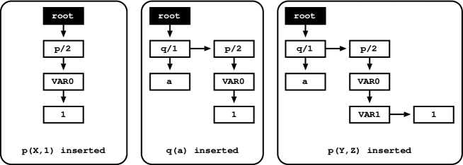
Figure 1: Using tries to represent terms

In variant-based tabling, each tabled predicate has a table entry data structure that contains information about the predicate and a pointer to the subgoal trie. A trie leaf node in the subgoal trie corresponds to a unique subgoal call and points to a data structure called the subgoal frame. The subgoal frame contains information about the subgoal, namely, the state of the subgoal and a pointer to the corresponding answer trie. In subsumption-based tabling based on the TST design, we have subsumptive subgoal frames, for subgoals that generate answers, and subsumed subgoal frames, for subgoals that consume answers from subsumptive subgoals [2].

Subsumptive subgoal frames are similar to variant subgoal frames, but they point to a time-stamped answer trie instead, which is an answer trie where each trie node is extended with timestamp information. Consider, for example, the subgoal call p(VAR0,VAR1) and the time-stamped answer trie in Fig. 3. The trie stores 2 answers, {f(x),1} inserted with timestamp 1 and {10,[]} inserted with timestamp 2. The root node contains the predicate timestamp and is incremented every time a new answer is inserted. Consider now that we insert the answer {f(y),1} (see Fig. 3). For this, we increment the predicate timestamp to 3 and then we set the timestamp of each node on the trie path of the new answer also to 3. Notice that if we look at leaf nodes we are able to discern in which order the answers were inserted, because each new answer is numbered incrementally.

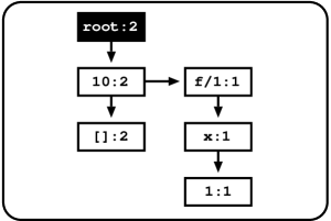
Figure 2: A time-stamped answer trie

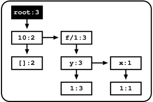
Figure 3: Inserting the answer {f(y),1}

Subsumed subgoal frames store a pointer to the corresponding subsumptive subgoal frame (the more general subgoal) instead of pointing to their own answer tries. The frames have a answer return list, a list of pointers to the relevant answers in the subsumptive answer trie and a consumer timestamp used for incremental retrieval of answers from the subsumptive answer trie. To consume answers, a subsumed subgoal first traverses its answer return list checking for more answers, and then executes a retrieval algorithm in the subsumptive answer trie in order to collect the answers with newer timestamps, which are then added to the answer return list. As an example, consider again the answer trie in Fig. 3 of the subgoal p(VAR0,VAR1). We are now interested in the incremental retrieval of relevant answers of the consumer subgoal p(VAR0,1). For this, we need to do a depth-first search on the answer trie using the consumer timestamp as a filter to ignore already retrieved answers, as we are only interested in answers that were added after the last retrieval operation. Assuming that the consumer timestamp was 1, we would retrieve the answer {f(y),1} and add it to the answer return list to be consumed next.

3 Retroactive Call Subsumption

RCS [6] is an extension to subsumption-based evaluation that enables answer reuse independently of the call order of the subgoals. While non-retroactive subsumption-based tabling only allows sharing of answers when a subsumed subgoal is called after a subsuming subgoal, RCS works around this drawback by selectively pruning the evaluation of subsumed subgoals and by turning them into consumers.

Let’s consider a subgoal $R$ that is subsumed by a subgoal $S$. To do retroactive evaluation, we must prune the evaluation of $R$, first by knowing which parts of the execution stacks are involved in its computation and then by transforming the choice point associated with $R$ into a consumer node, in such a way that it will consume answers from the subsuming subgoal $S$, instead of continuing the execution as a generator. A vital part in this process is that we need to know the set of answers $A_{old}$, that were already computed by $R$, so that, when we transform $R$ into a consumer we only consume the set of answers $A_{new}$, that will be created by $S$. In other words, we must ensure that the final set of answers $A$ for $R$ is $A=A_{new}\cup A_{old}$ with $A_{new}\cap A_{old}=\emptyset$. If we do not obey this principle, the evaluation will not be wrong, but several execution branches will be executed more than once, thus eliminating the potential advantage of RCS evaluation.

In RCS, we consider two types of pruning of subgoals. The first type is external pruning and occurs when $S$ is an external subgoal to the evaluation of $R$. The second one is internal pruning and occurs when $S$ is an internal subgoal to the evaluation of $R$. Both cases are very similar in terms of the challenges and problems that arise when doing pruning [6]. Here, we present an example of external pruning, that will help us to understand how RCS works, and then we focus on how the constraint $A_{new}\cap A_{old}=\emptyset$ presented before requires a better table space design than the one presented in the previous section. Consider thus the query goal ‘?- r(1,X), r(Y,Z)’ and the following program.

   :- use_retrosubsumptive_tabling r/2.
   r(1,a).
   r(Y,Z) :- ...

Execution starts by calling r(1,X), which creates a new generator to execute the program code, and a first answer for r(1,X), {X=a}, is found. In the continuation, r(Y,Z) is called, which will be a subsumptive subgoal for r(1,X). Thus, r(1,X) needs to be pruned and turned into a consumer of r(Y,Z). To prune, we turn the node of r(1,X) into a retroactive node that will later be transformed into either a consumer or a loader node, if r(Y,Z) does not complete or completes, respectively. In both cases, when backtracking to r(1,X), we need to consume only the new answers relevant to r(1,X) from r(Y,Z) that were not computed when r(1,X) was a generator (in this case, the answer {X=a}).

4 Single Time Stamped Trie

Once a pruned subgoal is reactivated and transformed into a consumer or loader node, it is important to avoid consuming answers that were found as a generator. In order to efficiently identify such answers, we designed the Single Time Stamped Trie (STST) table space.

In this new organization, each tabled predicate has two tries, the subgoal trie, as usual, and the STST, a time-stamped answer trie common to all subgoal calls for the predicate, while each subgoal frame has an answer return list that references the matching answers from the STST. Figure 4 illustrates an example of the new table space organization for a tabled predicate p/2 with the subgoals p(VAR0,1) and p(VAR0,VAR1) and the answers {f(x),1}, {10,[]} and {f(y),1}. This new organization reduces memory usage, since an answer is represented only once, and permits easy sharing of answers between subgoals, as the same answer can be referenced by multiple subgoal frames.

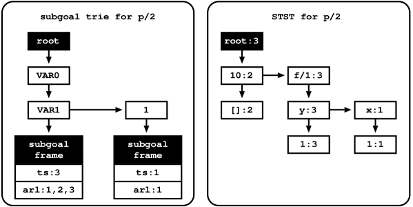
Figure 4: The new STST table space organization

For the subgoal frames, we have also extended them with a ts field that stores the timestamp of the last generated or consumed answer. At any time, the answers in the answer return list (field arl in Fig. 4) are thus the matching answers from the STST that have a timestamp between 0 and ts. When we turn a node from generator to consumer, we can collect new answers by using the timestamp stored in the corresponding subgoal frame, which was the timestamp of the last answer successfully inserted into the STST.

When a subsumed subgoal is pruned, we know its timestamp and we can easily turn it into a consumer, since now instead of inserting answers, the new consumer will now consume them from the STST, like in the TST design, by incrementally retrieving answers from it. Therefore, the cost of such transformation is very low given that both generators and consumers use an answer return list and a timestamp. If we had used the original TST design, the pruned subgoal would have its own answer trie, call it $T_{1}$, and we would need to, before consuming answers, check if the answers on $T_{1}$ have already appeared on the answer trie of the subsuming subgoal, call it $T_{2}$. Such a task is quite complex, since answers in $T_{1}$ are instances of the answers in $T_{2}$.

Notice that in both variant-based and subsumption-based tabling, only the substitutions for the variables in a subgoal call are stored in the answer tries [10]. For example, for the subgoal p(VAR0,1) and the answers {f(x),1} and {f(y),1}, only the substitutions {f(x)} and {f(y)} are stored, since during consumption of answers only the substitutions are used for unification. However, in the STST design, we cannot do this, since any subgoal of p/2 can use the answers stored in the answer trie, therefore we need to store all the subterms of each answer.

4.1 Inserting Answers

The insertion of answers in the STST works like the insertion of answers in standard TSTs, but special care must be taken when updating the ts field on the subgoal frames. When only one subgoal is adding answers to the STST, the ts field is incremented each time an answer is inserted. Repeated answers are easily recognized by testing if the answer is new or not by using the ts field. The problem arises when several subgoals are inserting answers, as it may be difficult to determine when an answer is new or repeated for a certain subgoal.

Let’s consider two subgoals of the same predicate $p$, $S_{1}$ and $S_{2}$, and their corresponding timestamps, $T_{1}$ and $T_{2}$. $S_{1}$ has found and inserted the first 3 answers ($T_{1}=3$) in the STST and $S_{2}$ then started evaluating and inserted the next 3 answers, answers 4, 5 and 6 ($T_{2}=6$). Now, when execution backtracks to $S_{1}$, answer 5 is found and, while it is already on the trie, it must be considered as a new answer for $S_{1}$.

By default, we could consider answer 5 as new, since $T_{1}$ is in the past ($T_{1}<5$). But this can also lead to problems if next we update $T_{1}$ to either 6 (the predicate timestamp) or 5 (the timestamp for answer 5). For example, if later, answer 4 is also found for $S_{1}$, it will be considered as a repeated answer during its insertion since now $T_{1}>4$. Therefore, we need a more complex mechanism to detect repeated subgoal answers.

In our approach, we use a pending answer index for each subgoal frame. This index contains all the answers that are older than the current subgoal frame timestamp field but that have not yet been found by the subgoal. It is built whenever the timestamp of the answer being inserted is younger than the subgoal frame timestamp, by collecting all the relevant answers in the STST with a timestamp younger than the current subgoal frame timestamp. Later, when an answer is found but is already on the trie, and therefore will have an older timestamp than the subgoal frame timestamp, we must lookup on the pending answer index to check if the answer is there. If so, we consider it a new answer and remove it from the index; if not, we consider it a repeated answer.

The pending answer index is implemented as a single linked list, but can be transformed into a hash table if the list reaches a certain threshold. In Fig. 5, we present the code for the stst_insert_answer() procedure, which given an answer and a subgoal frame, inserts the answer into the corresponding STST for the subgoal frame. The pseudo-code is organized into four cases:

1. Answers are inserted in order by the same subgoal. This is the most common situation.

2. The answer being inserted is the only answer in the STST that the current subgoal has still not considered. It is trivially marked as a new answer.

3. The timestamp of the answer being inserted is older than the subgoal frame timestamp. The pending answer index must be consulted.

4. The timestamp of the answer being inserted is younger than the subgoal frame timestamp $t$. We must collect all the relevant answers in the STST with a timestamp younger than $t$ (calling collect_relevant_answers()) and add them to the pending answer index, except for the current answer.

stst_insert_answer(answer, sg_fr) {
  table_entry = table_entry(sg_fr)
  stst = answer_trie(table_entry)
  old_ts = predicate_timestamp(stst)
  leaf_node = answer_check_insert(answer, stst)
  leaf_ts = timestamp(leaf_node)
  new_ts = predicate_timestamp(stst)

  if (new_ts == old_ts + 1 and ts(sg_fr) == old_ts)
    // case 1: incremental answer by the same subgoal
    ts(sg_fr) = new_ts
    return leaf_node
  else if (new_ts == old_ts == leaf_ts and ts(sg_fr) == new_ts - 1)
    // case 2: only answer still not considered by the current subgoal
    ts(sg_fr) == new_ts
    return leaf_node
  else if (leaf_ts <= ts(sg_fr))
    // case 3: answer with a past timestamp, check pending answer index
    if (is_in_pending_answer_index(leaf_node, sg_fr))
      remove_from_pending_answer_index(leaf_node, sg_fr)
      return leaf_node
    else
      return NULL
  else
    // case 4: answers were inserted by someone else
    ans_tpl = answer_template(sg_fr)
    pending_list = collect_relevant_answers(ts(sg_fr),ans_tpl,stst)
    remove_from_list(leaf_node, pending_list)
    add_to_pending_answer_index(pending_list, sg_fr)
    ts(sg_fr) = new_ts
    return leaf_node
}

Figure 5: Pseudo-code for procedure stst_insert_answer()

Note that when a generator subgoal frame is transformed into a consumer subgoal frame, we remove all the answers from the pending answer index and we safely insert them on the answer return list. With this, all the consumer mechanisms can be used as usual.

4.2 Reusing Answers

The STST approach also allows reusing answers when a new subgoal is called. As an example, consider that two unrelated (no subsumption involved) subgoals $S_{1}$ and $S_{2}$ are fully evaluated. If a subgoal $S$ is then called, it is possible that some of the answers on the STST match $S$ even if $S$ neither subsumes $S_{1}$ or $S_{2}$. Hence, instead of eagerly running the predicate clauses, we can start by loading the matching answers already on the STST, which can be enough if, for example, $S$ is pruned by a cut. This is a similar approach to the incomplete tabling technique for variant-based tabling [11].

While the reuse of answers has some advantages, it can also lead to redundant computations. This happens when the evaluation of $S$ generates more general answers than the ones initially stored on the STST. For an example, consider the retroactive tabled predicate p/2 with only one fact, p(X,a). If subgoal p(1,Y) is first called, the answer represented as {1,a} is added to the STST for p/2 and execution would succeed. If the subgoal p(X,Y) is then called, we would search the STST for relevant answers and the first answer would be {1,a}. If we ask for more answers, the system would return a new answer, {VAR0,a}, and add it to the STST. On the other hand, if we called p(X,Y) with an empty STST, only the answer {VAR0,a} would be returned.

4.3 Answer Templates

The answer template is a data structure that is built on the choice point stack and is pushed into the stack when a new subgoal, generator or consumer, is called. The contents of the answer template are the terms from the subgoal call that must be read when inserting a new answer, if a generator, or the terms from the subgoal call that must be unified when consuming answers, if a consumer.

On variant-based tabling, the answer template is just the set of variables found in the subgoal call, since we only store variable substitutions on the answer trie. For non-retroactive call by subsumption, where we use an answer trie per generator subgoal, the answer template for each consumer subgoal is built according to its generator subgoal. For example, if the subsumptive subgoal is p(1,f(X),Y) and the subsumed subgoal is p(1,f([A,B]),a(C)), the answer template for the subsumed subgoal will be {[A,B],a(C)}.

With RCS, the answer template is simply built by copying the full set of argument registers for the generator or consumer call. This is a very efficient operation compared to non-retroactive call by subsumption. Notice that we need the full answer template because the answers stored on the STST contain all the predicate arguments, hence the unification of matching answers must be seen as unifying against the most general subgoal.

4.4 Compiled Tries

Compiled tries are a well-known implementation mechanism in which we decorate a trie with WAM instructions when a subgoal completes in such a way that, instead of consuming answers one by one in a bottom-up fashion, we execute the trie instructions in order to consume answers incrementally in a top-down fashion, thus taking advantage of the nature of tries [10].

Our approach only compiles the STST when the most general subgoal is completed. This avoids problems when a subgoal is executing compiled code and another subgoal is inserting answers, leading to the loss of answers as hash tables can be dynamically created and expanded.

With this optimization, we can throw away the subgoal trie and the subgoal frames when the most general subgoal completes and the STST is compiled. Later, when a new subgoal call is made, we just build the answer template by copying the argument registers and then we execute the compiled trie, thus bypassing all the mechanisms of locating the subgoal on the subgoal trie, leading to memory and speedup gains.

5 Experimental Results

Previous experiments using the STST design for comparing RCS with non-retroactive call by subsumption, showed good results when executing programs that take advantage of RCS [6]. Despite these good results and while the STST presents some conveniences in implementing RCS, here we will focus in measuring the impact of having to store the complete answers on the STST, instead of storing only the variable substitutions, since it is more expensive to insert/load terms to/from the STST. To this purpose, we measured the overheads of several programs that stress this weakness, both in terms of time and space.

The environment for our experiments was a PC with a 2.66 GHz Intel Core(TM) 2 Quad CPU and 4 GBytes of memory running the Linux kernel 2.6.31 with YapTab 6.03. For benchmarking, we used six different versions of the well-known path/2 program, that computes the reachability between nodes in a graph, with several dataset configurations: chain, where each node $i$ connects with node $i+1$; cycle, like a chain, but the last node connects with the first; grid, where nodes are organized in a square configuration; pyramid, where nodes form a pyramid; and tree, a binary tree. To increase the size of the terms to be stored in the STST, we transformed, both the programs and datasets, to use a functor term in each argument, instead of simple integers. For example, a fact edge(3,4) was transformed into edge(f(3),f(4)) and the transformed version of the left_first (left recursion with the recursive clause first) path/2 program is:

   path(f(X),f(Z)) :- path(f(X),f(Y)), edge(f(Y),f(Z)).
   path(f(X),f(Z)) :- edge(f(X),f(Z)).

We experimented the six different versions of the path/2 program with different graph sizes for the datasets using a query goal, path(f(X),f(Y)), that does not take advantage of RCS evaluation, i.e., never calls more general subgoals after specific ones.

5.1 Execution Times

In Table 1, we present the execution times, in milliseconds, for RCS evaluation and the respective overheads for variant-based and non-retroactive subsumption-based tabling. Each execution time is the average of 3 runs.

Table 1: Execution times, in milliseconds, for RCS evaluation and the respective overheads for variant-based and non-retroactive subsumption-based tabling for the query goal path(f(X),f(Y)) in YapTab

Program/Dataset		YapTab
		RCS	RCS/Var	RCS/Sub
left_first	chain (2048)	812	1.21	1.30
	cycle (2048)	1,722	1.08	1.14
	grid (64)	17,261	1.38	1.17
	pyramid (1024)	869	1.18	1.23
	tree (65536)	573	1.23	1.17
	Average		1.22	1.20
left_last	chain (2048)	894	1.35	1.42
	cycle (2048)	1,794	1.13	1.29
	grid (64)	18,187	1.47	1.23
	pyramid (1024)	862	1.14	1.24
	tree (65536)	582	1.27	1.19
	Average		1.27	1.27
right_first	chain (4096)	4,004	1.21	1.21
	cycle (4096)	7,324	1.09	1.04
	grid (32)	1,130	1.27	1.29
	pyramid (2048)	3,172	1.17	1.10
	tree (32768)	300	1.15	1.04
	Average		1.18	1.14
right_last	chain (4096)	3,642	0.95	1.08
	cycle (4096)	7,965	0.98	1.12
	grid (32)	997	0.96	1.22
	pyramid (2048)	3,170	1.09	1.12
	tree (32768)	528	1.76	1.05
	Average		1.15	1.12
double_first	chain (256)	1,708	3.94	1.58
	cycle (256)	2,945	1.11	1.51
	grid (16)	3,936	1.53	1.53
	pyramid (256)	7,480	4.04	1.44
	tree (16384)	766	2.19	1.35
	Average		2.56	1.48
double_last	chain (256)	1,778	4.08	1.69
	cycle (256)	2,932	1.10	1.64
	grid (16)	3,956	1.57	1.54
	pyramid (256)	6,829	3.70	1.30
	tree (16384)	720	2.04	1.29
	Average		2.50	1.49
	Total Average		1.65	1.28

From these results, we can observe that, on total average for these set of benchmarks, the transformed path/2 program has an overhead of 65% and 28% when compared with variant-based and non-retroactive subsumption-based tabling, respectively. The insertion of new answers into the table space and the consumption of answers are the primary causes for these overheads. The programs with the worst overheads are double_first and double_last, with 48% and 49% of overhead against non-retroactive subsumption-based tabling. These programs also create the higher number of consumers, both variant consumers and subsumed consumers than any other benchmark in these experiments. The right_first and right_last only create subsumed consumers, and they have an overhead of 14% and 12%, respectively, against non-retroactive call by subsumption, which are the lowest overhead values. In the left_first and left_last programs, only one variant consumer is allocated, however, on average, they perform worse than the right versions.

We thus argue that the number of consumer nodes can greatly reduce the applicability and performance of the STST table space organization when the operation of loading an answer from the trie is more expensive. While this situation seems disadvantageous, execution time can be reduced if another subgoal call appears (for example path(X,Y)) where it is possible to reuse the answers from the table before executing the predicate clauses.

5.2 Memory Usage

We executed the previous benchmarks and measured the number of answer trie nodes stored for each program. Table 2 presents such numbers for RCS evaluation and the relative numbers for variant and subsumption-based tabling. The programs left, right and double are the left, right and double versions of the path/2 program (note that the number of stored trie nodes is the same for both the versions of the path/2 program, with the recursive clause first or with the recursive clause last).

Table 2: Number of stored answer trie nodes for RCS evaluation and the relative numbers for variant-based and non-retroactive subsumption-based tabling for the query goal path(f(X),f(Y)) in YapTab

Program/Dataset		YapTab
		#RCS	Var/RCS	Sub/RCS
left	chain (2048)	2,100,233	0.99902	0.99902
	cycle (2048)	4,200,450	0.99902	0.99902
	grid (64)	16,789,506	0.99951	0.99951
	pyramid (1024)	1,576,457	0.99870	0.99870
	tree (65536)	983,056	0.96665	0.96665
	Average		0.99258	0.99258
right	chain (4096)	8,398,847	1.99756	0.99902
	cycle (4096)	16,789,506	1.99902	0.99951
	grid (32)	1,051,650	1.99610	0.99805
	pyramid (2048)	6,302,719	1.99675	0.99870
	tree (32768)	491,520	1.76667	0.90000
	Average		1.95122	0.97906
double	chain (256)	26,387	2.48365	0.87490
	cycle (256)	36,844	3.57141	0.89333
	grid (16)	59,028	2.22920	0.82586
	pyramid (256)	56,638	3.47583	0.95187
	tree (16384)	213,008	1.88449	0.96148
	Average		2.72892	0.90149
	Total Average		1.89091	0.95771

From these results we can observe that, on total average for this set of benchmarks, the variant-based table design requires 1.89 times more memory space than the STST table space organization. In particular, for the double program, these differences are higher because in the variant-based design there are more generator subgoal calls and thus more answer tries are created.

When comparing RCS to the non-retroactive subsumption-based engine, the latter only stores, on total average for this set of benchmarks, around 4% less trie nodes than RCS evaluation, even if the f/1 functor terms need to be stored in the STST. This is easily understandable because the first f/1 functor term is only represented once, at the top of the STST, and then there is one second f/1 functor for each node in the graph, therefore, the total number of functors stored in the STST is insignificant when compared to the total number of terms stored in the trie. Also note that, for the double benchmarks, the datasets used are small if compared to the datasets used for the other benchmarks, but the space overhead is more significant (18% in the worst case). We thus argue that the cost of the extra space needed to store terms in the STST is less significant as more terms are stored in the tries.

6 Conclusions

We presented a new table space organization that is particularly well suited to be used with Retroactive Call Subsumption. Our proposal uses ideas from the original TST design and innovates by having only a single answer trie per predicate, making it easier to share answers across subgoals for the same predicate. We presented the challenges when using a single answer trie and how they have been solved, for example, with the use of pending answer indices. Moreover, we think that the new design should not be very difficult to port to other tabling engines, since it uses the trie data structure extended with timestamp information.

Our experiments with RCS showed promising results when used with programs that take advantages of the new mechanisms. In this paper, we benchmarked and discussed the overhead in terms of time and space when storing and loading complete answers, instead of using variable substitutions, for programs that do not takes advantage of RCS evaluation, i.e., that never call more general subgoals after specific ones. Our results show that the time overhead can be noticeable, however, in terms of space, the number of extra trie nodes appears to be low.

References

- [1] Chen, W., Warren, D.S.: Tabled Evaluation with Delaying for General Logic Programs. Journal of the ACM 43(1) (1996) 20–74
- [2] Johnson, E., Ramakrishnan, C.R., Ramakrishnan, I.V., Rao, P.: A Space Efficient Engine for Subsumption-Based Tabled Evaluation of Logic Programs. In: Fuji International Symposium on Functional and Logic Programming. Number 1722 in LNCS, Springer-Verlag (1999) 284–300
- [3] Rao, P., Sagonas, K., Swift, T., Warren, D.S., Freire, J.: XSB: A System for Efficiently Computing Well-Founded Semantics. In: International Conference on Logic Programming and Non-Monotonic Reasoning. Number 1265 in LNCS, Springer-Verlag (1997) 431–441
- [4] Rao, P., Ramakrishnan, C.R., Ramakrishnan, I.V.: A Thread in Time Saves Tabling Time. In: Joint International Conference and Symposium on Logic Programming, The MIT Press (1996) 112–126
- [5] Johnson, E.: Interfacing a Tabled-WAM Engine to a Tabling Subsystem Supporting Both Variant and Subsumption Checks. In: Conference on Tabulation in Parsing and Deduction. (2000)
- [6] Cruz, F., Rocha, R.: Retroactive Subsumption-Based Tabled Evaluation of Logic Programs. In: European Conference on Logics in Artificial Intelligence. Number 6341 in LNAI, Springer-Verlag (2010) 130–142
- [7] Rocha, R., Silva, F., Santos Costa, V.: YapTab: A Tabling Engine Designed to Support Parallelism. In: Conference on Tabulation in Parsing and Deduction. (2000) 77–87
- [8] Rocha, R., Silva, F., Santos Costa, V.: On applying or-parallelism and tabling to logic programs. Theory and Practice of Logic Programming 5(1 & 2) (2005) 161–205
- [9] Freire, J., Swift, T., Warren, D.S.: Beyond Depth-First: Improving Tabled Logic Programs through Alternative Scheduling Strategies. In: International Symposium on Programming Language Implementation and Logic Programming. Number 1140 in LNCS, Springer-Verlag (1996) 243–258
- [10] Ramakrishnan, I.V., Rao, P., Sagonas, K., Swift, T., Warren, D.S.: Efficient Access Mechanisms for Tabled Logic Programs. Journal of Logic Programming 38(1) (1999) 31–54
- [11] Rocha, R.: Handling Incomplete and Complete Tables in Tabled Logic Programs. In: International Conference on Logic Programming. Number 4079 in LNCS, Springer-Verlag (2006) 427–428