The next-to-leading order jet vertex for Mueller-Navelet and forward jets revisited

F. Caporale^1†, D.Yu. Ivanov^2¶, B. Murdaca^1†, A. Papa^1†, A. Perri^1†

¹ Dipartimento di Fisica, Università della Calabria,

and Istituto Nazionale di Fisica Nucleare, Gruppo collegato di Cosenza,

I-87036 Arcavacata di Rende, Cosenza, Italy

² Sobolev Institute of Mathematics and Novosibirsk State University,

630090 Novosibirsk, Russia

We recalculate, within the BFKL approach and at the next-to-leading order, the jet vertex relevant for the production of Mueller-Navelet jets in proton collisions and of forward jets in DIS. We consider both processes with incoming quark and gluon. The starting point is the definition of quark and gluon impact factors in the BFKL approach. Following this procedure we show explicitly that all infrared divergences cancel when renormalized parton densities are considered. We compare our results for the vertex with the former calculation of Refs. [1, 2].

$\begin{array}[]{ll}{}^{\dagger}\mbox{{\it e-mail address:}}&\mbox{francesco.caporale, beatrice.murdaca, alessandro.papa,}\\ &\mbox{amedeo.perri\ @fis.unical.it}\\ {}^{\P}\mbox{{\it e-mail address:}}&\mbox{d-ivanov@math.nsc.ru}\\ \end{array}$

1 Introduction

The Mueller-Navelet jet production process [3] was suggested as an ideal tool to study the Regge limit of perturbative Quantum ChromoDynamics (QCD) in proton-proton (or proton-antiproton) collisions. It is an inclusive process

$$p(p_{1})+p(p_{2})\to J_{1}(k_{J,1})+J_{2}(k_{J,2})+X\,,$$ (1)

where two hard jets $J_{1}$ and $J_{2}$ are produced (the transverse momenta of jets are much larger than the QCD scale, $\vec{k}_{J,1}^{2}\sim\vec{k}_{J,2}^{2}\gg\Lambda_{\rm QCD}^{2}$) in the kinematical region where the jets are separated by a large interval of rapidity, $\Delta y\gg 1$. This regime requires large center of mass energy $s$ of the proton collisions, $s=2p_{1}\cdot p_{2}\gg\vec{k}_{J\,1,2}^{2}$, since $\Delta y\sim\ln{s/\vec{k}^{2}_{J\,1,2}}$. It can be studied experimentally at modern high energy hadron colliders, LHC and Tevatron.

The BFKL approach [4] is the most suitable framework for the theoretical description of the high-energy limit of hard or semi-hard processes. At high $s$, large logarithms of the energy compensate the small coupling and must be resummed at all orders of the perturbative series. The BFKL approach provides a systematic way to perform the resummation in the leading logarithmic approximation (LLA), which means resummation of all terms $(\alpha_{s}\ln(s))^{n}$, and in the next-to-leading logarithmic approximation (NLA), which means resummation of all terms $\alpha_{s}(\alpha_{s}\ln(s))^{n}$.

In the BFKL approach, both in the LLA and in the NLA, the high-energy scattering amplitudes are expressed by a suitable factorization of a process-independent part, the Green’s function for the interaction of two Reggeized gluons, and process-dependent terms, the so-called impact factors of the colliding particles (see, for instance, [5]). The Green’s function is determined through the BFKL equation, whose kernel is known at the next-to-leading order (NLO) [6, 7]. The impact factors of the colliding particle are a necessary ingredient for the complete description of a process in the BFKL approach and, therefore, to get a contact with phenomenology. The only impact factors calculated so far with NLO accuracy are those for colliding quark and gluons [8, 9, 10, 11], for forward jet production [1, 2], for the $\gamma^{*}\to\gamma^{*}$ transition [12], and for the $\gamma^{*}$ to light vector meson transition at leading twist [13].

The D0 collaboration at Tevatron [14] observed power-like rise of the Mueller-Navelet jet cross section with energy, though the D0 results revealed an even stronger rise than predicted by LLA BFKL calculations. Besides the cross section measurement, it was suggested to study a less inclusive observable, such as the decorrelation of jets in the relative azimuthal angle. The D0 experiment [15] found less decorrelation than predicted by LLA calculations [16, 17].

Important improvements were made toward the description of the process within NLA accuracy. Effects related with QCD running coupling were studied in [18, 19]. In [20, 21, 22] the full NLO Green’s function was implemented, but the jets impact factors were taken into account at the leading order only.

Recently the results of a complete NLA analysis of the process (1) were reported [23], which incorporates NLO corrections to both the BFKL Green’s function and the jets impact factors, calculated earlier in [1, 2]. The authors of [23] found that for kinematics typical of the LHC experiment the effect of NLO corrections to the jet impact factors is very important, of the same order as the one obtained from the NLO correction to Green’s function. This observation is similar to one obtained earlier in the NLA analysis of the diffractive double $\rho$-electroproduction [24]. Another important conclusion of [23] is that the results for Mueller-Navelet jet observables obtained within complete BFKL NLA analysis appeared to be very close to the one calculated in the conventional collinear factorization at the NLO, with the only exception of the ratio between the azimuthal angular moments $\langle\cos(2\phi)\rangle/\langle\cos\phi\rangle$.

In our opinion it would be important to have an independent calculation of Mueller-Navelet jet observables in NLA. The aim of the present paper is the calculation of NLO correction to the jet impact factor in order to have an independent check of the results of [1, 2]. In many technical steps we follow closely the method used in [1, 2], but we will take advantage of starting from the general definition for the impact factors at NLO, see [5], which allows us to come to the results more shortly.

The paper is organized as follows. In the next Section we will present the factorization structure of the cross section, recall the definition of BFKL impact factor and discuss the treatment of the divergences arising in the calculation; in Section 3 we give the derivation of the quark contribution to the impact factor; Section 4 is devoted to the calculation of the gluon part; finally, in Section 5 we summarize our results and make a comparison to the ones of [1, 2].

2 General framework

The state of the jets can be described completely by their rapidities, $y_{1,2}$, and transverse momenta, $\vec{k}_{J,1}$ and $\vec{k}_{J,2}$. We denote the azimuthal angles of the produced jets as $\phi_{1}$ and $\phi_{2}$. It is convenient to define the Sudakov decomposition for the jets momenta. For a jet in the fragmentation region of the proton with momentum $p_{1}$, one has

$$k_{J,1}=x_{J,1}p_{1}+\frac{\vec{k}^{2}_{J,1}}{x_{J,1}s}p_{2}+k_{J,1\,\perp}\ ,\quad\quad\quad k_{J,1\,\perp}^{2}=-\vec{k}^{2}_{J,1}\ ,$$ (2)

where we assume $p_{1}^{2}=p_{2}^{2}=0$ neglecting the proton mass and the longitudinal fraction $x_{J,1}={\cal O}(1)$ is related to the jet rapidity in the center of mass system by

$$y_{1}=\frac{1}{2}\ln\frac{x_{J,1}^{2}s}{\vec{k}_{J,1}^{2}}\;,\quad\quad dy_{1}=\frac{dx_{J,1}}{x_{J,1}}\;.$$

In QCD collinear factorization the cross section of the process reads

$$\frac{d\sigma}{dx_{J,1}dx_{J,2}d^{2}\vec{k}_{J,1}d^{2}\vec{k}_{J,2}}=\sum_{i,j=q,\bar{q},g}\int\limits^{1}_{0}\int\limits^{1}_{0}dx_{1}dx_{2}f_{i}(x_{1},\mu)f_{j}(x_{2},\mu)\frac{d\hat{\sigma}_{i,j}(x_{1}x_{2}s,\mu)}{dx_{J,1}dx_{J,2}d^{2}\vec{k}_{J,1}d^{2}\vec{k}_{J,2}}\;,$$ (3)

where the $i,j$ indices specify parton types (quarks $q=u,d,s$; antiquarks $\bar{q}=\bar{u},\bar{d},\bar{s}$; or gluon $g$), $f_{i}(x,\mu)$ denotes the initial proton parton density function (PDF), the longitudinal fractions of the partons involved in the hard subprocess are $x_{1,2}$, $\mu$ is the factorization scale and $d\hat{\sigma}_{i,j}(x_{1}x_{2}s,\mu)$ is the partonic cross section for the production of jets, and $\hat{s}=x_{1}x_{2}s$ is the energy of parton-parton collision. At lowest order each jet is represented by a single parton having high transverse momentum, and the partonic subprocess is given by an elementary two-to-two scattering. In the discussed Mueller-Navelet kinematics the higher order contributions to the partonic cross section have to be resummed using BFKL approach. Such resummation at NLA accuracy depends on the details of jet definition (jet algorithm) and will be specified later.

A convenient starting point for our discussion is the case of inclusive forward parton-parton scattering, considered in $D=4+2\varepsilon$ dimensions to regularize the appearing divergences. Due to the optical theorem, the cross section is related to the imaginary part of the forward parton-parton scattering amplitude,

$$\hat{\sigma}=\frac{{\cal I}m_{s}A}{\hat{s}}\ ,$$ (4)

which is given in the BFKL approach at NLA by

$${\cal I}m_{s}{\cal A}=\frac{\hat{s}}{(2\pi)^{D-2}}\int\frac{d^{D-2}\vec{q}_{1}}{\vec{q}_{1}^{\,\,2}}\Phi_{P,1}(\vec{q}_{1},s_{0})\int\frac{d^{D-2}\vec{q}_{2}}{\vec{q}_{2}^{\,\,2}}\Phi_{P,2}(-\vec{q}_{2},s_{0})\int\limits^{\delta+i\infty}_{\delta-i\infty}\frac{d\omega}{2\pi i}\left(\frac{\hat{s}}{s_{0}}\right)^{\omega}G_{\omega}(\vec{q}_{1},\vec{q}_{2})\,,$$ (5)

where the Green’s function obeys the BFKL equation

$$\omega\,G_{\omega}(\vec{q}_{1},\vec{q}_{2})=\delta^{(D-2)}(\vec{q}_{1}-\vec{q}_{2})+\int d^{D-2}\vec{q}\,K(\vec{q}_{1},\vec{q})\,G_{\omega}(\vec{q},\vec{q}_{1})\;,$$ (6)

and $\Phi_{P,1}(\vec{q}_{1},s_{0})$,  $\Phi_{P,2}(-\vec{q}_{2},s_{0})$ are the parton impact factors calculated separately for the cases of massless quark and gluon in [8, 9, 10]. Here $\vec{q}_{1}$, $\vec{q}_{2}$ are the transverse momenta of the Reggeized gluons, the energy scale parameter $s_{0}$ is arbitrary, the amplitude, indeed, does not depend on its choice within NLA accuracy.

2.1 Parton impact factors

In this subsection we review the definition of the impact factors in NLO.

Both the kernel of the equation for the Green’s function and the parton impact factors can be expressed in terms of the gluon Regge trajectory,

$$j(t)\;=\;1\>+\>\omega(t)\;,$$ (7)

and the effective vertices for the Reggeon-parton interaction.

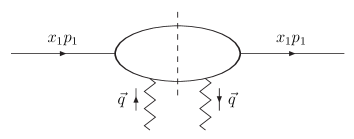
Figure 1: Schematic representation of the forward parton impact factor. Here $p_{1}$ is the proton momentum, $x_{1}$ is the fraction of proton momentum carried by the parton and $\vec{q}$ is the transverse momentum of the incoming Reggeized gluon.

To be more specific, we will give below the formulae for the case of forward quark impact factor. We start with the LO, where the quark impact factors are given by

$$\Phi_{q}^{(0)}(\vec{q}\,)\;=\;\sum_{\{a\}}\>\int\>\frac{dM_{a}^{2}}{2\pi}\>\Gamma_{aq}^{(0)}(\vec{q}\,)\>[\Gamma_{aq}^{(0)}(\vec{q}\,)]^{*}\>d\rho_{a}\;,$$ (8)

where $\vec{q}$ is the Reggeon transverse momentum, and $\Gamma^{(0)}_{aq}$ denotes the Reggeon-quark vertices in the LO or Born approximation. The sum $\{a\}$ is over all intermediate states $a$ which contribute to the $q\rightarrow q$ transition. The phase space element $d\rho_{a}$ of a state $a$, consisting of particles with momenta $\ell_{n}$, is ($p_{q}$ is initial quark momentum)

$$d\rho_{a}\;=\;(2\pi)^{D}\>\delta^{(D)}\left(p_{q}+q-\sum_{n\in a}\ell_{n}\right)\>\prod_{n\in a}\>\frac{d^{D-1}\ell_{n}}{(2\pi)^{D-1}2E_{n}}\;,$$ (9)

while the remaining integration in (8) is over the squared invariant mass of the state $a$,

$$M_{a}^{2}\;=\;(p_{q}+q)^{2}\;.$$

In the LO the only intermediate state which contributes is a one-quark state, $\{a\}=q$. The integration in Eq. (8) with the known Reggeon-quark vertices $\Gamma_{qq}^{(0)}$ is trivial and the quark impact factor reads

$$\Phi_{q}^{(0)}(\vec{q}\,)\;=g^{2}\frac{\sqrt{N_{c}^{2}-1}}{2N_{c}}\;,$$ (10)

where $g$ is QCD coupling, $\alpha_{s}=g^{2}/(4\pi)$, $N_{c}=3$ is the number of QCD colors.

In the NLO the expression (8) for the quark impact factor has to be changed in two ways. First one has to take into account the radiative corrections to the vertices,

$$\Gamma_{qq}^{(0)}\to\Gamma_{qq}=\Gamma_{qq}^{(0)}+\Gamma_{qq}^{(1)}\;.$$

Secondly, in the sum over $\{a\}$ in (8), we have to include more complicated states which appear in the next order of perturbative theory. For the quark impact factor this is a state with an additional gluon, $a=qg$. However, the integral over $M_{a}^{2}$ becomes divergent when an extra gluon appears in the final state. The divergence arises because the gluon may be emitted not only in the fragmentation region of initial quark, but also in the central rapidity region. The contribution of the central region must be subtracted from the impact factor, since it is to be assigned in the BFKL approach to the Green’s function. Therefore the result for the forward quark impact factor, see [9] and Fig. 1, reads

$$\Phi_{q}(\vec{q}\,,s_{0})=\left(\frac{s_{0}}{\vec{q}^{\>2}}\right)^{\omega(-\vec{q}^{\>2})}\>\sum_{\{a\}}\>\int\>\frac{dM_{a}^{2}}{2\pi}\>\Gamma_{aq}(\vec{q}\,)\>[\Gamma_{aq}(\vec{q}\,)]^{*}\>d\rho_{a}\>\theta(s_{\Lambda}-M_{a}^{2})$$

$$-\frac{1}{2}\int d^{D-2}k\frac{\vec{q}^{\,\,2}}{\vec{k}^{\,2}}\Phi_{q}^{(0)}(\vec{k})\mathcal{K}_{r}^{(0)}(\vec{k},\vec{q}\,)\ln\left(\frac{s_{\Lambda}^{2}}{(\vec{k}-\vec{q}\,)^{2}s_{0}}\right)\;,$$ (11)

where the intermediate parameter $s_{\Lambda}$ should go to infinity. The second term in the r.h.s. of (2.1) is the subtraction of the gluon emission in the central rapidity region. The dependence on $s_{\Lambda}$ vanishes because of the cancellation between the first and second terms. $K_{r}^{(0)}$ is the part of LO BFKL kernel related to real gluon production

$$K_{r}^{(0)}(\vec{k},\vec{q}\,)\;=\;\frac{2g^{2}N_{c}}{(2\pi)^{D-1}}\frac{1}{(\vec{k}-\vec{q}\,)^{2}}\;.$$ (12)

The factor in (2.1) which involves the Regge trajectory arises from the change of energy scale ($\vec{q}^{\>2}\to s_{0}$) in the vertices $\Gamma$. The trajectory function $\omega(t)$ can be taken here in the one-loop approximation ($t=-\vec{q}^{\,\,2}$),

$$\omega(t)\;=\;\frac{g^{2}t}{(2\pi)^{D-1}}\frac{N_{c}}{2}\int\frac{d^{D-2}k}{\vec{k}^{2}(\vec{q}-\vec{k})^{2}}\;=\;-\;g^{2}N_{c}\frac{\Gamma(1-\varepsilon)}{(4\pi)^{D/2}}\frac{\Gamma^{2}(\varepsilon)}{\Gamma(2\varepsilon)}(\vec{q}^{\,\,2})^{\varepsilon}\;.$$ (13)

In the Eqs. (8) and (2.1) we suppress for shortness the color indices (for the explicit form of the vertices see [8, 9]). The gluon impact factor $\Phi_{g}(\vec{q}\,)$ is defined similarly. In the gluon case only the single-gluon intermediate state contributes in the LO, $a=g$, which results in

$$\Phi_{g}^{(0)}(\vec{q}\,)\;=\frac{C_{A}}{C_{F}}\Phi_{q}^{(0)}(\vec{q}\,)\;,$$ (14)

here $C_{A}=N_{c}$ and $C_{F}=(N^{2}_{c}-1)/(2N_{c})$. Whereas in NLO additional two-gluon, $a=gg$, and quark-antiquark, $a=q\bar{q}$, intermediate states have to be taken into account in the calculation of the gluon impact factor.

2.2 Jet impact factor

Similarly to the parton-parton scattering (5) one can represent the resummed jet cross section in the form

$$\frac{d\sigma}{dJ_{1}dJ_{2}}=\frac{1}{(2\pi)^{D-2}}\!\int\frac{d^{D-2}\vec{q}_{1}}{\vec{q}_{1}^{\,\,2}}\frac{d\Phi_{J,1}(\vec{q}_{1},s_{0})}{dJ_{1}}\!\int\frac{d^{D-2}\vec{q}_{2}}{\vec{q}_{2}^{\,\,2}}\frac{d\Phi_{J,2}(-\vec{q}_{2},s_{0})}{dJ_{2}}\!\!\int\limits^{\delta+i\infty}_{\delta-i\infty}\frac{d\omega}{2\pi i}\left(\frac{\hat{s}}{s_{0}}\right)^{\omega}\!G_{\omega}(\vec{q}_{1},\vec{q}_{2})\,,$$ (15)

where we introduce jet impact factors differential with respect to the variables parameterizing the jet phase space,

$$dJ_{1}\equiv dx_{J,1}d^{D-2}k_{J,1}\;,\quad\quad dJ_{2}\equiv dx_{J,2}d^{D-2}k_{J,2}\;.$$

Following [1] we consider our process in the frame of a generic and infrared safe jet algorithm. In practice, this is done by introducing into the integration over the partonic phase space a suitably defined function which identifies the jet momentum with the momentum of one parton or with the sum of the two or more parton momenta when the jet is originated from the a multi-parton intermediate state. In our accuracy the jet can be formed by one parton in LO and by one or two partons when the process is considered in NLO. In the simplest case, the jet momentum is identified with the momentum of the parton in the intermediate state $k$ by the following jet function [25]:

$$S_{J}^{(2)}(\vec{k};x)=\delta(x-x_{J})\delta^{(D-2)}(\vec{k}-\vec{k}_{J})\;.$$ (16)

In the more complicated case when the jet originates from a state of two partons with momenta $k_{1}$ and $k_{2}$, we need another function $S_{J}^{(3)}$, whose explicit form is specific for the chosen jet algorithm. An example of jet selection function in the case of the cone algorithm is the following [25]:

$$S_{J}^{(3,\rm{cone})}(\vec{k}_{2},\vec{k}_{1},x\beta_{1};x) = S_{J}^{(2)}(\vec{k}_{2};x(1-\beta_{1}))\Theta\left(\left[\Delta y^{2}+\Delta\phi^{2}\right]-\left[\frac{|\vec{k}_{1}|+|\vec{k}_{2}|}{\max(|\vec{k}_{1}|,|\vec{k}_{2}|)}R_{\mbox{\scriptsize{cone}}}\right]^{2}\right)$$

$$+ S_{J}^{(2)}(\vec{k}_{1};x\beta_{1})\Theta\left(\left[\Delta y^{2}+\Delta\phi^{2}\right]-\left[\frac{|\vec{k}_{1}|+|\vec{k}_{2}|}{\max(|\vec{k}_{1}|,|\vec{k}_{2}|)}R_{\mbox{\scriptsize{cone}}}\right]^{2}\right)$$

$$+ S_{J}^{(2)}(\vec{k}_{1}+\vec{k}_{2};x)\Theta\left(\left[\frac{|\vec{k}_{1}|+|\vec{k}_{2}|}{\max(|\vec{k}_{1}|,|\vec{k}_{2}|)}R_{\mbox{\scriptsize{cone}}}\right]^{2}-\left[\Delta y^{2}+\Delta\phi^{2}\right]\right)\;,$$

where the Sudakov decomposition of the parton momenta

$$k_{1} = x\beta_{1}p_{1}+\frac{\vec{k}_{1}^{\,2}}{x\beta_{1}s}p_{2}+k_{1_{\perp}}\;,\;\;\;\;\;k_{1}^{2}=0\;,$$ (18)

$$k_{2} = x\beta_{2}p_{1}+\frac{\vec{k}_{2}^{\,2}}{x\beta_{2}s}p_{2}+k_{2_{\perp}}\;,\;\;\;\;\;k_{2}^{2}=0\;,$$ (19)

is used, with $\beta_{1}+\beta_{2}=1$ and $\vec{k}_{1}+\vec{k}_{2}=\vec{q}$, owing to momentum conservation in the partonic subprocess. $R_{\mbox{\scriptsize{cone}}}$ in (2.2) is the cone-size parameter, $\Delta y$ and $\Delta\phi$ are the difference of rapidity and azimuthal angle in the two parton state, respectively:

$$\Delta y=\ln\left(\frac{1-\beta_{1}}{\beta_{1}}\frac{|\vec{k}_{1}|}{|\vec{k}_{2}|}\right)\;,\;\;\;\;\;\Delta\phi=\arccos\frac{\vec{k}_{1}\cdot\vec{k}_{2}}{\sqrt{\vec{k}_{1}^{\,2}\vec{k}_{2}^{\,2}}}\;.$$ (20)

The three terms in $S_{J}^{(3,{\rm cone})}$ represent the case in which the jet is formed by the parton $k_{2}$ or the parton $k_{1}$ or both, respectively.

In the generic case, the following relations for the jet function must be fulfilled in order the jet algorithm be infrared safe:

$$S_{J}^{(3)}(\vec{k}_{2},\vec{k}_{1},x\beta_{1};x) \longrightarrow S_{J}^{(2)}(\vec{k}_{2};x)\;,\hskip 59.75095pt\vec{k}_{1}\rightarrow 0\;,\;\;\;\beta_{1}\rightarrow 0\;,$$

$$S_{J}^{(3)}(\vec{k}_{2},\vec{k}_{1},x\beta_{1};x) \longrightarrow S_{J}^{(2)}(\vec{k}_{1}+\vec{k}_{2};x)\;,\;\;\;\;\;\;\;\;\;\;\vec{k}_{1}\beta_{2}\rightarrow\vec{k}_{2}\beta_{1}\;,$$

$$S_{J}^{(3)}(\vec{k}_{2},\vec{k}_{1},x\beta_{1};x) \longrightarrow S_{J}^{(2)}(\vec{k}_{2};x(1-\beta_{1}))\;,\;\;\;\;\;\vec{k}_{1}\rightarrow 0\;,$$ (21)

$$S_{J}^{(3)}(\vec{k}_{2},\vec{k}_{1},x\beta_{1};x) \longrightarrow S_{J}^{(2)}(\vec{k}_{1};x\beta_{1})\;,\hskip 48.36958pt\vec{k}_{2}\rightarrow 0\;.$$

Such reduction of $S^{(3)}_{J}\to S^{(2)}_{J}$ is required in order that the singular contributions generated by the real emission be proportional to the lowest order cross section. These contributions are canceled with the soft and collinear singularities arising from the virtual corrections and the collinear counterterms coming from the PDFs renormalization.

Besides, we assume that the jet selection function $S_{J}^{(3)}$ is symmetric under the exchange of the final state parton kinematic variables, $\beta_{1}\leftrightarrow\beta_{2}$ and $\vec{k}_{1}\leftrightarrow\vec{k}_{2}$,

$$S_{J}^{(3)}(\vec{k}_{2},\vec{k}_{1},x\beta_{1};x)=S_{J}^{(3)}(\vec{k}_{1},\vec{k}_{2},x\beta_{2};x)\;.$$ (22)

The collinear counterterms appear due to the replacement of the bare PDFs by the renormalized physical quantities which obey DGLAP evolution equations, in the $\overline{\rm MS}$ factorization scheme:

$$f_{q}(x)=f_{q}(x,\mu_{F})-\frac{\alpha_{s}}{2\pi}\left(\frac{1}{\hat{\varepsilon}}+\ln\frac{\mu_{F}^{2}}{\mu^{2}}\right)\int\limits^{1}_{x}\frac{dz}{z}\left[P_{qq}(z)f_{q}(\frac{x}{z},\mu_{F})+P_{qg}(z)f_{g}(\frac{x}{z},\mu_{F})\right]\;,$$

$$f_{g}(x)=f_{g}(x,\mu_{F})-\frac{\alpha_{s}}{2\pi}\left(\frac{1}{\hat{\varepsilon}}+\ln\frac{\mu_{F}^{2}}{\mu^{2}}\right)\int\limits^{1}_{x}\frac{dz}{z}\left[P_{gq}(z)f_{q}(\frac{x}{z},\mu_{F})+P_{gg}(z)f_{g}(\frac{x}{z},\mu_{F})\right]\;,$$ (23)

where $\frac{1}{\hat{\varepsilon}}=\frac{1}{\varepsilon}+\gamma_{E}-\ln(4\pi)\approx\frac{\Gamma(1-\varepsilon)}{\varepsilon(4\pi)^{\varepsilon}}$ and the DGLAP splitting functions are:

$$P_{qq}(z) = C_{F}\left(\frac{1+z^{2}}{1-z}\right)_{+}=C_{F}\left[\frac{1+z^{2}}{(1-z)_{+}}+\frac{3}{2}\delta(1-z)\right]\;,$$ (24)

$$P_{qg}(z) = T_{R}\left[z^{2}+(1-z)^{2}\right]\;,\;\;\;\mbox{with}\ T_{R}=\frac{1}{2}\;,$$ (25)

$$P_{gg}(z) = 2C_{A}\left(\frac{z}{(1-z)_{+}}+\frac{(1-z)}{z}+z(1-z)\right)+\frac{(11C_{A}-4N_{F}T_{R})}{6}\delta(1-z)\;,$$ (26)

$$P_{gq}(z) = C_{F}\frac{\left[1+(1-z)^{2}\right]}{z}\;;$$ (27)

here the plus-prescription is defined by

$$\int_{a}^{1}dx\frac{F(x)}{(1-x)_{+}}=\int_{a}^{1}dx\frac{F(x)-F(1)}{1-x}-\int_{0}^{a}dx\frac{F(1)}{1-x}\;.$$ (28)

The other counterterm is related with QCD charge renormalization, in the $\overline{\rm MS}$ scheme:

$$\alpha_{s}=\alpha_{s}(\mu_{R})\left[1+\frac{\alpha_{s}(\mu_{R})}{4\pi}\left(\frac{11C_{A}}{3}-\frac{2N_{F}}{3}\right)\left(\frac{1}{\hat{\varepsilon}}+\ln\frac{\mu_{R}^{2}}{\mu^{2}}\right)\right]\;.$$ (29)

Having the results for the lowest order parton impact factors (10) and (14), we get the jet impact factor at the LO level as

$$\frac{d\Phi^{(0)}_{J}(\vec{q}\,)}{dJ}=g^{2}\frac{\sqrt{N_{c}^{2}-1}}{2N_{c}}\int_{0}^{1}dx\left(\frac{C_{A}}{C_{F}}f_{g}(x)+\sum_{a=q,\bar{q}}f_{a}(x)\right)S_{J}^{(2)}(\vec{q};x)\;,$$ (30)

given as the sum of the gluon and all possible quark and antiquark PDFs contributions. Substituting here the bare QCD coupling and bare PDFs by the renormalized ones, we obtain the following expressions for the counterterms:

$$\frac{d\Phi_{J}(\vec{q}\,)|_{\rm{charge\ c.t.}}}{dJ}=\frac{\alpha_{s}}{2\pi}\left(\frac{1}{\hat{\varepsilon}}+\ln\frac{\mu_{R}^{2}}{\mu^{2}}\right)\left(\frac{11C_{A}}{6}-\frac{N_{F}}{3}\right)\,\Phi^{(0)}_{q}$$

$$\times\int_{0}^{1}dx\left(\frac{C_{A}}{C_{F}}f_{g}(x)+\sum_{a=q,\bar{q}}f_{a}(x)\right)S_{J}^{(2)}(\vec{q};x)$$ (31)

for the charge renormalization, and

$$\frac{d\Phi_{J}(\vec{q}\,)|_{\rm{collinear\ c.t.}}}{dJ}=-\frac{\alpha_{s}}{2\pi}\left(\frac{1}{\hat{\varepsilon}}+\ln\frac{\mu_{F}^{2}}{\mu^{2}}\right)\Phi^{(0)}_{q}\int\limits^{1}_{0}\,dx\,S_{J}^{(2)}(\vec{q}\,;x)\int\limits^{1}_{x}\frac{dz}{z}$$

$$\times\left[\sum_{a=q,\bar{q}}\left(P_{qq}(z)f_{a}\left(\frac{x}{z}\right)+P_{qg}(z)f_{g}\left(\frac{x}{z}\right)\right)+\frac{C_{A}}{C_{F}}\left(P_{gg}(z)f_{g}\left(\frac{x}{z}\right)+P_{gq}(z)\sum_{a=q,\bar{q}}f_{a}\left(\frac{x}{z}\right)\right)\right]$$ (32)

for the collinear counterterm. The latter can be rewritten in the form

$$\frac{d\Phi_{J}(\vec{q}\,)|_{\rm{collinear\ c.t.}}}{dJ}=-\frac{\alpha_{s}}{2\pi}\left(\frac{1}{\hat{\varepsilon}}+\ln\frac{\mu_{F}^{2}}{\mu^{2}}\right)\Phi^{(0)}_{q}\int\limits^{1}_{0}\,d\beta\,\int\limits^{1}_{0}\,dx\,S_{J}^{(2)}(\vec{q}\,;\beta x)$$

$$\times\left[\sum_{a=q,\bar{q}}\left(P_{qq}(\beta)f_{a}\left(x\right)+P_{qg}(\beta)f_{g}\left(x\right)\right)+\frac{C_{A}}{C_{F}}\left(P_{gg}(\beta)f_{g}\left(x\right)+P_{gq}(\beta)\sum_{a=q,\bar{q}}f_{a}\left(x\right)\right)\right]\;.$$ (33)

Besides, we present the expression for the BFKL counterterm which, in accordance to the second line of Eq. (2.1), provides the subtraction of the gluon radiation in the central rapidity region:

$$\frac{d\Phi_{J}(\vec{q}\,)|_{\rm{BFKL\ c.t.}}}{dJ} = -\Phi^{(0)}_{q}\frac{C_{A}\,g^{2}}{(2\pi)^{D-1}}\int_{0}^{1}dx\left(\frac{C_{A}}{C_{F}}f_{g}(x)+\sum_{a=q,\bar{q}}f_{a}(x)\right)$$ (34)

$$\times \int d^{D-2}\vec{k}\ \frac{\vec{q}^{\,\,2}}{\vec{k}^{\,2}(\vec{k}-\vec{q}\,)^{2}}\ln\left(\frac{s_{\Lambda}^{2}}{s_{0}\ \vec{k}^{2}}\right)\,S_{J}^{(2)}(\vec{q}-\vec{k};x)\;.$$

Now we have all the necessary ingredients to perform our calculation of the NLO corrections to the jet impact factor. As a starting point for our consideration we will use the results of [8, 9] for the partonic amplitudes obtained in the calculation of partonic impact factors, introducing there the appropriate jet functions: $S^{(2)}_{J}$ for the amplitudes with one-parton state in the case of one-loop virtual corrections and $S^{(3)}_{J}$ for the cases with two partons in the final state (real emission), in order to define the corresponding contribution to jet cross sections.

For shortness we will present intermediate results for $V$ structures defined always as

$$\frac{d\Phi^{(1)}_{J}(\vec{q}\,)}{dJ}\,\equiv\,\frac{\alpha_{s}}{2\pi}\,\Phi^{(0)}_{q}\,V(\vec{q}\,)\;.$$ (35)

We will consider separately the subprocesses initiated by the quark and the gluon PDFs and denote

$$V=V_{q}+V_{g}\,.$$ (36)

3 NLA jet impact factor: the quark contribution

We start with the case of incoming quark (see Fig. 2).

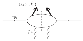
Figure 2: Schematic representation of the jet vertex for the case of quark in the initial state. Here $p_{1}$ is the proton momentum, $x$ is the fraction of proton momentum carried by the quark, $x_{J}p_{1}$ is the longitudinal jet momentum, $\vec{k}_{J}$ is the transverse jet momentum and $\vec{q}$ is the transverse momentum of the incoming Reggeized gluon.

3.1 Virtual correction

Virtual corrections are the same as in the case of the inclusive quark impact factor [8, 9, 10]:

$$V_{q}^{(V)}(\vec{q}\,)=-\frac{\Gamma[1-\varepsilon]}{\varepsilon\,(4\pi)^{\varepsilon}}\frac{\Gamma^{2}(1+\varepsilon)}{\Gamma(1+2\varepsilon)}\left(\vec{q}^{\,\,2}\right)^{\varepsilon}\int_{0}^{1}dx\sum_{a=q,\bar{q}}f_{a}(x)\,S_{J}^{(2)}(\vec{q}\,;x)$$

$$\times\left\{C_{F}\left(\frac{2}{\varepsilon}-\frac{4}{1+2\varepsilon}+1\right)\right.-N_{F}\frac{1+\varepsilon}{(1+2\varepsilon)(3+2\varepsilon)}+C_{A}\left(\ln\frac{s_{0}}{\vec{q}^{\,\,2}}+\psi(1-\varepsilon)-2\psi(\varepsilon)+\psi(1)\right.$$

$$\left.\left.+\frac{1}{4(1+2\varepsilon)(3+2\varepsilon)}-\frac{2}{\varepsilon(1+2\varepsilon)}-\frac{7}{4(1+2\varepsilon)}-\frac{1}{2}\right)\right\}\;.$$ (37)

Here and in what follows we put the arbitrary scale of dimensional regularization equal to unity, $\mu=1$. We expand (37) in $\varepsilon$ and get

$$V_{q}^{(V)}(\vec{q}\,)=-\frac{\Gamma[1-\varepsilon]}{\varepsilon\,(4\pi)^{\varepsilon}}\frac{\Gamma^{2}(1+\varepsilon)}{\Gamma(1+2\varepsilon)}\left(\vec{q}^{\,\,2}\right)^{\varepsilon}\int_{0}^{1}dx\sum_{a=q,\bar{q}}f_{a}(x)\,S_{J}^{(2)}(\vec{q}\,;x)$$

$$\times\left[C_{F}\left(\frac{2}{\varepsilon}-3\right)-\frac{N_{F}}{3}+C_{A}\left(\ln\frac{s_{0}}{\vec{q}^{\,\,2}}+\frac{11}{6}\right)\right.$$

$$\left.+\,\varepsilon\left\{8\,C_{F}+\frac{5N_{F}}{9}-C_{A}\left(\frac{85}{18}+\frac{\pi^{2}}{2}\right)\right\}\right]+{\cal O}(\varepsilon)\,.$$ (38)

3.2 Real corrections

For the incoming quark case, real corrections originate from the quark-gluon intermediate state. We denote the momentum of the gluon by $k$, then the momentum of the quark is $q-k$; the longitudinal fraction of the gluon momentum is denoted by $\beta x$. Thus, the real contribution has the form [8, 9, 10, 26]

$$V^{(R)}_{q}(\vec{q}\,) = \frac{1}{(4\pi)^{\varepsilon}}\int_{0}^{1}dx\sum_{a=q,\bar{q}}f_{a}(x)\int\frac{d^{D-2}\vec{k}}{\pi^{1+\varepsilon}}\int_{\beta_{0}}^{1}d\beta\,{\cal P}_{gq}(\varepsilon,\beta)$$ (39)

$$\times \frac{\vec{q}^{\>2}}{\vec{k}^{\,2}(\vec{q}-\vec{k})^{2}(\vec{k}-\beta\vec{q}\,)^{2}}\left\{C_{F}\beta^{2}(\vec{q}-\vec{k})^{2}+C_{A}(1-\beta)\vec{k}\cdot(\vec{k}-\beta\vec{q}\,)\right\}$$

$$\times S_{J}^{(3)}\left(\vec{q}-\vec{k},\vec{k},x\beta;x\right)\;,$$

where

$$\beta_{0}=\frac{\vec{k}^{\,2}}{s_{\Lambda}}\;,\;\;\;\;\;\;\;{\cal P}_{gq}(\varepsilon,\beta)=\frac{1+(1-\beta)^{2}+\varepsilon\beta^{2}}{\beta}\;.$$

The low limit in the $\beta$-integration appears due to the restriction on the invariant mass of intermediate state, which enters the definition (2.1) of NLO impact factor. Since

$$M^{2}_{qg}=\frac{\vec{k}^{2}}{\beta}+\frac{(\vec{q}-\vec{k})^{2}}{1-\beta}-\vec{q}^{\,\,2}\;,\;\;\;\;M^{2}_{qg}\leq s_{\Lambda}\;,$$

and assuming $s_{\Lambda}\to\infty$, we obtain that $\beta\geq\beta_{0}$.

We consider separately the term proportional to $C_{F}$ and to $C_{A}$.

The $C_{F}$-term is not singular for $\beta\to 0$, therefore the limit $s_{\Lambda}\to\infty$, or $\beta_{0}\to 0$, can be safely taken. We get

$$V^{(R)(C_{F})}_{q}(\vec{q}\,) = \frac{C_{F}}{(4\pi)^{\varepsilon}}\int_{0}^{1}dx\sum_{a=q,\bar{q}}f_{a}(x)\int\frac{d^{D-2}\vec{k}}{\pi^{1+\varepsilon}}\int_{0}^{1}d\beta\,{\cal P}_{gq}(\varepsilon,\beta)$$ (40)

$$\times \frac{\vec{q}^{\>2}\beta^{2}}{\vec{k}^{\,2}(\vec{k}-\beta\vec{q}\,)^{2}}S_{J}^{(3)}\left(\vec{q}-\vec{k},\vec{k},x\beta;x\right)\;.$$

In order to isolate all divergences, it is convenient to perform the change of variable $\vec{k}=\beta\vec{l}$ and to present the integral in the form

$$V^{(R)(C_{F})}_{q}(\vec{q}\,) = \frac{C_{F}}{(4\pi)^{\varepsilon}}\int_{0}^{1}dx\sum_{a=q,\bar{q}}f_{a}(x)\int_{0}^{1}d\beta\,{\cal P}_{gq}(\varepsilon,\beta)\beta^{2\varepsilon}$$

$$\times \int\frac{d^{D-2}\vec{l}}{\pi^{1+\varepsilon}}\frac{\vec{q}^{\>2}}{\vec{l}^{\>2}+(\vec{l}-\vec{q}\,)^{2}}\left[\frac{1}{(\vec{l}-\vec{q}\,)^{2}}+\frac{1}{\vec{l}^{\>2}}\right]S_{J}^{(3)}\left(\vec{q}-\beta\vec{l},\beta\vec{l},x\beta;x\right)\;.$$

The soft divergence appears for $\beta\rightarrow 0$; in this region we can introduce the counterterm

$$V^{(R)(C_{F},{\rm soft})}_{q}(\vec{q}\,) = \frac{C_{F}}{(4\pi)^{\varepsilon}}\int_{0}^{1}dx\sum_{a=q,\bar{q}}f_{a}(x)\int_{0}^{1}d\beta\,\frac{2}{\beta^{1-2\varepsilon}}$$

$$\times \int\frac{d^{D-2}\vec{l}}{\pi^{1+\varepsilon}}\frac{\vec{q}^{\>2}}{\vec{l}^{\>2}+(\vec{l}-\vec{q}\,)^{2}}\left[\frac{1}{(\vec{l}-\vec{q}\,)^{2}}+\frac{1}{\vec{l}^{\>2}}\right]S_{J}^{(2)}\left(\vec{q};x\right)\;,$$

which equals

$$V^{(R)(C_{F},{\rm soft})}_{q}(\vec{q}\,)=\frac{2C_{F}}{\varepsilon}\frac{\Gamma[1-\varepsilon]}{\varepsilon\,(4\pi)^{\varepsilon}}\frac{\Gamma^{2}(1+\varepsilon)}{\Gamma(1+2\varepsilon)}\left(\vec{q}^{\,\,2}\right)^{\varepsilon}\int_{0}^{1}dx\sum_{a=q,\bar{q}}f_{a}(x)\,S_{J}^{(2)}(\vec{q}\,;x)\;.$$ (43)

Collinear divergences arise for $\vec{l}-\vec{q}=0$ and for $\vec{l}=0$; in these regions we can isolate the two following counterterms:

$$V^{(R)(C_{F},{\rm coll_{1}})}_{q}(\vec{q}\,) = \frac{C_{F}}{(4\pi)^{\varepsilon}}\int\frac{d^{D-2}\vec{l}}{\pi^{1+\varepsilon}(\vec{l}-\vec{q}\,)^{2}}\Theta(\Lambda^{2}-(\vec{l}-\vec{q}\,)^{2})$$

$$\times \int_{0}^{1}d\beta\beta^{2\varepsilon}\left[{\cal P}_{gq}(\varepsilon,\beta)-\frac{2}{\beta}\right]\int_{0}^{1}dx\sum_{a=q,\bar{q}}f_{a}(x)S_{J}^{(2)}(\vec{q}\,;x)\;,$$

$$V^{(R)(C_{F},{\rm coll_{2}})}_{q}(\vec{q}\,) = \frac{C_{F}}{(4\pi)^{\varepsilon}}\int\frac{d^{D-2}\vec{l}}{\pi^{1+\varepsilon}\vec{l}^{\>2}}\Theta(\Lambda^{2}-\vec{l}^{\>2})\int_{0}^{1}dx\sum_{a=q,\bar{q}}f_{a}(x)$$

$$\times \int_{0}^{1}d\beta\ \beta^{2\varepsilon}\left[S_{J}^{(2)}(\vec{q}\,;x(1-\beta)){\cal P}_{gq}(\varepsilon,\beta)-\frac{2}{\beta}S_{J}^{(2)}(\vec{q}\,;x)\right]\;.$$

In both these expressions we have introduced an arbitrary cutoff parameter $\Lambda$ and subtracted the soft divergence. After a simple calculation we obtain

$$V^{(R)(C_{F},{\rm coll_{1}})}_{q}(\vec{q}\,) = \frac{\Gamma[1-\varepsilon]}{\varepsilon\,(4\pi)^{\varepsilon}}\frac{\Gamma^{2}(1+\varepsilon)}{\Gamma(1+2\varepsilon)}\left(\Lambda^{2}\right)^{\varepsilon}\int_{0}^{1}dx\sum_{a=q,\bar{q}}f_{a}(x)S_{J}^{(2)}(\vec{q}\,;x)$$ (46)

$$\times C_{F}\left[-\frac{3}{2}+4\varepsilon\right]+\mathcal{O}(\varepsilon)\;.$$

The term $V^{(R)(C_{F},{\rm coll_{2}})}_{q}$ can be rewritten in the following form:

$$V^{(R)(C_{F},{\rm coll_{2}})}(\vec{q}\,) = \frac{\Gamma[1-\varepsilon]}{\varepsilon\,(4\pi)^{\varepsilon}}\frac{\Gamma^{2}(1+\varepsilon)}{\Gamma(1+2\varepsilon)}\left(\Lambda^{2}\right)^{\varepsilon}\int_{0}^{1}dx\sum_{a=q,\bar{q}}f_{a}(x)\left\{-\frac{3}{2}C_{F}S_{J}^{(2)}(\vec{q}\,;x)\right.$$ (47)

$$+ \int_{0}^{1}d\beta\left[P_{qq}(\beta)+\,2\varepsilon(1+\beta^{2})\left(\frac{\ln(1-\beta)}{1-\beta}\right)_{+}C_{F}+\varepsilon\,C_{F}(1-\beta)\right]$$

$$\times \left.S_{J}^{(2)}(\vec{q}\,;x\beta)\right\}+\mathcal{O}(\varepsilon)\;,$$

where we performed the change of variable $\beta\to 1-\beta$, used the plus-prescription (28) and the expansion

$$(1-\beta)^{2\varepsilon-1}=\frac{1}{2\varepsilon}\delta(1-\beta)+\frac{1}{(1-\beta)_{+}}+2\varepsilon\left(\frac{\ln(1-\beta)}{1-\beta}\right)_{+}+\mathcal{O}(\varepsilon^{2})\;.$$

Finally, we can define the term

$$V^{(R)(C_{F},{\rm finite})}_{q}=V^{(R)(C_{F})}_{q}-V^{(R)(C_{F},{\rm soft})}_{q}-V^{(R)(C_{F},{\rm coll_{1}})}_{q}-V^{(R)(C_{F},{\rm coll_{2}})}_{q}\;,$$ (48)

which can be calculated at $\varepsilon=0$. We remark that $V^{(R)(C_{F},{\rm finite})}_{q}$ and $V^{(R)(C_{F},{\rm cool_{1,2}})}_{q}$ depend on the cutoff $\Lambda$, but in the total expression $V^{(R)(C_{F})}_{q}$ this dependence disappears.

The part proportional to $C_{A}$ in the r.h.s. of Eq. (39) reads

$$V_{q}^{(R)(C_{A})}(\vec{q}\,) = \frac{1}{(4\pi)^{\varepsilon}}\int_{0}^{1}dx\sum_{a=q,\bar{q}}f_{a}(x)\int\frac{d^{D-2}\vec{k}}{\pi^{1+\varepsilon}}\int_{\beta_{0}}^{1}d\beta\,{\cal P}_{gq}(\varepsilon,\beta)$$ (49)

$$\times \vec{q}^{\>2}C_{A}\,\frac{(1-\beta)\vec{k}\cdot(\vec{k}-\beta\vec{q}\,)}{\vec{k}^{\,2}(\vec{q}-\vec{k})^{2}(\vec{k}-\beta\vec{q}\,)^{2}}S_{J}^{(3)}\left(\vec{q}-\vec{k},\vec{k},x\beta;x\right)\;.$$

The collinear singularity appears at $\vec{k}-\vec{q}\,\to 0$; in this region we can introduce the counterterm

$$V_{q}^{(R)(C_{A},{\rm coll})}(\vec{q}\,) = \frac{C_{A}}{(4\pi)^{\varepsilon}}\int\frac{d^{D-2}\vec{k}}{\pi^{1+\varepsilon}(\vec{q}-\vec{k})^{2}}\Theta\left(\Lambda^{2}-(\vec{k}-\vec{q}\,)^{2}\right)$$

$$\times \int_{0}^{1}dx\sum_{a=q,\bar{q}}f_{a}(x)\int_{0}^{1}\,d\beta\,{\cal P}_{gq}(\varepsilon,\beta)\,S_{J}^{(2)}(\vec{q}\,;x\beta)$$

$$= \frac{\Gamma[1-\varepsilon]}{\varepsilon\,(4\pi)^{\varepsilon}}\frac{\Gamma^{2}(1+\varepsilon)}{\Gamma(1+2\varepsilon)}\left(\Lambda^{2}\right)^{\varepsilon}$$

$$\times \int_{0}^{1}dx\sum_{a=q,\bar{q}}f_{a}(x)\int_{0}^{1}\,d\beta\,\left[\frac{C_{A}}{C_{F}}P_{gq}(\beta)+\,\varepsilon\,C_{A}\,\beta\,\right]\,S_{J}^{(2)}(\vec{q}\,;x\beta)+\mathcal{O}(\varepsilon)\;,$$

where $\beta_{0}$ has been set equal to zero since the expression is finite in the $\beta\rightarrow 0$ limit and, again, the cutoff $\Lambda$ was introduced. Another singularity appears when $\beta\rightarrow 0$, actually at any value of gluon transverse momentum $\vec{k}$. In this region $S_{J}^{(3)}\left(\vec{q}-\vec{k},\vec{k},x\beta;x\right)\to S_{J}^{(2)}\left(\vec{q}-\vec{k};x\right)$ and it is convenient to introduce the counterterm

$$V_{q}^{(R)(C_{A},{\rm soft})}(\vec{q}\,) = \frac{C_{A}}{(4\pi)^{\varepsilon}}\int_{0}^{1}dx\sum_{a=q,\bar{q}}f_{a}(x)\int\frac{d^{D-2}\vec{k}}{\pi^{1+\varepsilon}}\int_{\beta_{0}}^{1}d\beta\,\frac{2}{\beta}$$ (51)

$$\times \vec{q}^{\>2}\,\frac{(1-\beta)\vec{k}\cdot(\vec{k}-\beta\vec{q}\,)}{\vec{k}^{\,2}(\vec{q}-\vec{k})^{2}(\vec{k}-\beta\vec{q}\,)^{2}}S_{J}^{(2)}\left(\vec{q}-\vec{k};x\right)$$

$$= \frac{C_{A}}{(4\pi)^{\varepsilon}}\int_{0}^{1}dx\sum_{a=q,\bar{q}}f_{a}(x)\int\frac{d^{D-2}\vec{k}}{\pi^{1+\varepsilon}}\int_{\beta_{0}}^{1}d\beta\,\frac{2}{\beta}$$

$$\times \,\frac{\vec{q}^{\>2}\Theta[(1-\beta)|\vec{k}|-\beta|\vec{q}-\vec{k}|]}{\vec{k}^{2}(\vec{q}-\vec{k})^{2}}S_{J}^{(2)}\left(\vec{q}-\vec{k};x\right)\;,$$

where the averaging over the relative angle between the vectors $\vec{k}$ and $\vec{q}-\vec{k}$ has been performed. The integration over $\beta$ gives the following result for the counterterm:

$$V_{q}^{(R)(C_{A},{\rm soft})}(\vec{q}\,) = \frac{C_{A}}{(4\pi)^{\varepsilon}}\int_{0}^{1}dx\sum_{a=q,\bar{q}}f_{a}(x)\int\frac{d^{D-2}\vec{k}}{\pi^{1+\varepsilon}}\,\frac{\vec{q}^{\>2}}{\vec{k}^{2}(\vec{q}-\vec{k})^{2}}$$ (52)

$$\times \ln\frac{s^{2}_{\Lambda}}{\vec{k}^{2}(|\vec{k}|+|\vec{q}-\vec{k}|)^{2}}\,\,S_{J}^{(2)}\left(\vec{q}-\vec{k};x\right)\;.$$

The finite part of the real corrections proportional to $C_{A}$ is therefore defined by

$$V_{q}^{(R)(C_{A},{\rm finite})}=V_{q}^{(R)(C_{A})}-V_{q}^{(R)(C_{A},{\rm coll})}-V_{q}^{(R)(C_{A},{\rm soft})}\;.$$ (53)

When the quark part of BFKL counterterm, given in (34),

$$V_{q}^{(C)}(\vec{q}\,)=-\frac{C_{A}}{(4\pi)^{\varepsilon}}\int_{0}^{1}dx\sum_{a=q,\bar{q}}f_{a}(x)\int\frac{d^{D-2}\vec{k}}{\pi^{1+\varepsilon}}\ln\left(\frac{s_{\Lambda}^{2}}{s_{0}\vec{k}^{2}}\right)\frac{\vec{q}^{\>2}}{\vec{k}^{\,2}(\vec{q}-\vec{k})^{2}}S_{J}^{(2)}\left(\vec{q}-\vec{k}\,;\,x\right)\,,$$ (54)

is combined with $V_{q}^{(R)(C_{A},{\rm soft})}$ given in (52), we see that the dependence on $s_{\Lambda}$ disappears, as expected, and we get

$$V_{q}^{(R)(C_{A},{\rm soft})}(\vec{q}\,)+V_{q}^{(C)}(\vec{q}\,)$$ (55)

$$=\frac{C_{A}}{(4\pi)^{\varepsilon}}\int_{0}^{1}dx\sum_{a=q,\bar{q}}f_{a}(x)\int\frac{d^{D-2}\vec{k}}{\pi^{1+\varepsilon}}\frac{\vec{q}^{\>2}}{\vec{k}^{\,2}(\vec{k}-\vec{q}\,)^{2}}\ln\left(\frac{s_{0}}{(|\vec{k}|+|\vec{q}-\vec{k}|)^{2}}\right)\ S^{(2)}_{J}(\vec{q}-\vec{k};x)\;.$$

3.3 Final result for the quark in the initial state

We collect first the contributions given in (38), (43), (46), (47) and (3.2):

$$V_{q}^{(1)}(\vec{q}\,)\equiv\left(V_{q}^{(V)}+V_{q}^{(R)(C_{F},{\rm soft})}+V_{q}^{(R)(C_{F},{\rm coll_{1}})}+V_{q}^{(R)(C_{F},{\rm coll_{2}})}+V_{q}^{(R)(C_{A},{\rm coll})}\right)(\vec{q}\,)$$

$$= \frac{\Gamma[1-\varepsilon]}{\varepsilon\,(4\pi)^{\varepsilon}}\frac{\Gamma^{2}(1+\varepsilon)}{\Gamma(1+2\varepsilon)}\int_{0}^{1}dx\,\sum_{a=q,\bar{q}}f_{a}(x)$$

$$\times \left\{\left[\left(\vec{q}^{\,\,2}\right)^{\varepsilon}\left(\frac{N_{F}}{3}-C_{A}\ln\left(\frac{s_{0}}{\vec{q}^{\>2}}\right)-\frac{11C_{A}}{6}\right)\,+\,\varepsilon\left(C_{A}\left(\frac{85}{18}+\frac{\pi^{2}}{2}\right)-\frac{5}{9}N_{F}\right.\right.\right.$$

$$+ \left.\left.C_{F}\left(3\ln\frac{\vec{q}^{\>2}}{\Lambda^{2}}-4\right)\right)\right]\ S^{(2)}_{J}(\vec{q}\,;x)$$

$$+ \left(\Lambda^{2}\right)^{\varepsilon}\int_{0}^{1}d\beta\left[P_{qq}(\beta)+\frac{C_{A}}{C_{F}}P_{gq}(\beta)\right]\ S^{(2)}_{J}(\vec{q}\,;x\beta)$$

$$+ \left.\varepsilon\int_{0}^{1}d\beta\left[2(1+\beta^{2})\left(\frac{\ln(1-\beta)}{1-\beta}\right)_{+}C_{F}+C_{F}(1-\beta)+C_{A}\beta\right]\ S^{(2)}_{J}(\vec{q}\,;x\beta)\,\right\}+\mathcal{O}(\varepsilon)\;.$$

Then, we collect the finite contributions, given in Eqs. (48) and (53), transforming them to the form used in [1]:

$$V_{q}^{(2)}(\vec{q}\,)\equiv\left(V_{q}^{(R)(C_{F},{\rm finite})}+V_{q}^{(R)(C_{A},{\rm finite})}\right)(\vec{q}\,)$$

$$=\int_{0}^{1}dx\,\sum_{a=q,\bar{q}}f_{a}(x)\left[C_{F}\int_{0}^{1}d\beta\frac{1}{(1-\beta)_{+}}(1+\beta^{2})\int\frac{d^{2}\vec{l}}{\pi\,\vec{l}^{\>2}}\left[\frac{\vec{q}^{\,\,2}}{\vec{l}^{2}+(\vec{q}-\vec{l})^{2}}\right.\right.$$

$$\left\{S_{J}^{(3)}(\vec{q}-(1-\beta)\vec{l},(1-\beta)\vec{l},x(1-\beta);x)+S_{J}^{(3)}(\vec{q}\beta+(1-\beta)\vec{l},(1-\beta)(\vec{q}-\vec{l}),x(1-\beta);x)\right\}$$

$$\biggl{.}-\Theta(\Lambda^{2}-\vec{l}^{\>2})\left\{S_{J}^{(2)}(\vec{q}\,;x\beta)+S_{J}^{(2)}(\vec{q}\,;x)\right\}\biggr{]}$$

$$+\,C_{A}\,\int\frac{d^{2}\vec{k}}{\pi\vec{k}^{2}}\int_{0}^{1}d\beta\left\{\frac{1+(1-\beta)^{2}}{\beta}\right.$$ (57)

$$\times\left[\frac{\vec{q}^{\>2}(1-\beta)(\vec{q}-\vec{k})\cdot(\vec{q}(1-\beta)-\vec{k})}{(\vec{q}-\vec{k})^{2}(\vec{q}(1-\beta)-\vec{k})^{2}}S_{J}^{(3)}(\vec{k},\vec{q}-\vec{k},x\beta;x)\right.$$

$$\left.\left.\left.-\Theta(\Lambda^{2}-\vec{k}^{2})S_{J}^{(2)}\left(\vec{q}\,;x\beta\right)\right]-\frac{2\,\vec{q}^{\>2}\Theta[(1-\beta)|\vec{q}-\vec{k}|-\beta|\vec{k}|]}{\beta(\vec{q}-\vec{k})^{2}}S_{J}^{(2)}(\vec{k};x)\right\}\right]+\mathcal{O}(\varepsilon)\,.$$

Besides, we define

$$V_{q}^{(3)}(\vec{q}\,)\equiv\left(V_{q}^{(R)(C_{A},{\rm soft})}+V_{q}^{(C)}\right)(\vec{q}\,)\;,$$

given in Eq. (55).

Another contribution originates from the collinear and charge renormalization counterterms, see Eqs. (31) and (33),

$$V_{q}^{(4)}(\vec{q}\,)=\frac{\Gamma[1-\varepsilon]}{\varepsilon\,(4\pi)^{\varepsilon}}\int_{0}^{1}dx\,\sum_{a=q,\bar{q}}f_{a}(x)\left[\left(\mu_{R}^{2}\right)^{\varepsilon}\left(\frac{11C_{A}}{6}-\frac{N_{F}}{3}\right)S_{J}^{(2)}\left(\vec{q}\,;x\right)\right.$$

$$\left.-\left(\mu_{F}^{2}\right)^{\varepsilon}\int_{0}^{1}d\beta\left[P_{qq}(\beta)+\frac{C_{A}}{C_{F}}P_{gq}(\beta)\right]\ S^{(2)}_{J}(\vec{q}\,;x\beta)\right]\;.$$ (58)

Finally, the quark part of the jet impact factor is given by the sum of the above four contributions and can be presented as the sum of two terms:

$$V_{q}^{(I)}(\vec{q}\,)=\int_{0}^{1}dx\,\sum_{a=q,\bar{q}}f_{a}(x)\left[\frac{C_{A}}{(4\pi)^{\varepsilon}}\int\frac{d^{D-2}\vec{k}}{\pi^{1+\varepsilon}}\frac{\vec{q}^{\>2}}{\vec{k}^{\,2}(\vec{k}-\vec{q}\,)^{2}}\ln\frac{s_{0}}{(|\vec{k}|+|\vec{q}-\vec{k}|)^{2}}\ S^{(2)}_{J}(\vec{k};x)\right.$$

$$\left.-C_{A}\ln\left(\frac{s_{0}}{\vec{q}^{\>2}}\right)\left(\vec{q}^{\,\,2}\right)^{\varepsilon}\frac{\Gamma[1-\varepsilon]}{\varepsilon\,(4\pi)^{\varepsilon}}\frac{\Gamma^{2}(1+\varepsilon)}{\Gamma(1+2\varepsilon)}S^{(2)}_{J}(\vec{q}\,;x)\right]\;.$$ (59)

and

$$V_{q}^{(II)}(\vec{q}\,)=V_{q}^{(2)}(\vec{q}\,)+\int_{0}^{1}dx\,\sum_{a=q,\bar{q}}f_{a}(x)$$ (60)

$$\times\left\{\left[\left(\frac{N_{F}}{3}-\frac{11C_{A}}{6}\right)\,\ln\frac{\vec{q}^{\,\,2}}{\mu_{R}^{2}}\,+\,C_{A}\left(\frac{85}{18}+\frac{\pi^{2}}{2}\right)-\frac{5}{9}N_{F}\right.\right.+\left.C_{F}\left(3\ln\frac{\vec{q}^{\>2}}{\Lambda^{2}}-4\right)\right]\ S^{(2)}_{J}(\vec{q}\,;x)$$

$$+\int_{0}^{1}d\beta\left[P_{qq}(\beta)+\frac{C_{A}}{C_{F}}P_{gq}(\beta)\right]\,\ln\frac{\Lambda^{2}}{\mu_{F}^{2}}\,\ S^{(2)}_{J}(\vec{q}\,;x\beta)$$

$$+\left.\int_{0}^{1}d\beta\left[2\left(\frac{\ln(1-\beta)}{1-\beta}\right)_{+}(1+\beta^{2})\,C_{F}+C_{F}(1-\beta)+C_{A}\beta\right]\ S^{(2)}_{J}(\vec{q}\,;x\beta)\,\right\}\;.$$

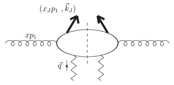
Figure 3: Schematic representation of the jet vertex for the case of gluon in the initial state. Here $p_{1}$ is the proton momentum, $x$ is the fraction of proton momentum carried by the gluon, $x_{J}p_{1}$ is the longitudinal jet momentum, $\vec{k}_{J}$ is the transverse jet momentum and $\vec{q}$ is the transverse momentum of the incoming Reggeized gluon.

4 NLA jet impact factor: the gluon contribution

We consider now the case of incoming gluon (see Fig. 3).

4.1 Virtual corrections

Virtual corrections are the same as in the case of the inclusive gluon impact factor [8, 9, 10]:

$$V_{g}^{(V)}(\vec{q}) = -\frac{\Gamma[1-\varepsilon]}{\varepsilon\,(4\pi)^{\varepsilon}}\frac{\Gamma^{2}(1+\varepsilon)}{\Gamma(1+2\varepsilon)}\left(\vec{q}^{\,\,2}\right)^{\varepsilon}\,\int_{0}^{1}dx\,\frac{C_{A}}{C_{F}}\,f_{g}(x)\,S_{J}^{(2)}(\vec{q}\,;x)$$

$$\times \left[C_{A}\ln\left(\frac{s_{0}}{\vec{q}^{\>2}}\right)+C_{A}\left(\frac{2}{\varepsilon}-\frac{11+9\varepsilon}{2(1+2\varepsilon)(3+2\varepsilon)}\right.\right.$$

$$+ \left.\frac{N_{F}}{C_{A}}\frac{(1+\varepsilon)(2+\varepsilon)-1}{(1+\varepsilon)(1+2\varepsilon)(3+2\varepsilon)}+\psi(1)+\psi(1-\varepsilon)-2\psi(1+\varepsilon)\right)$$

$$+ \left.C_{A}\frac{\varepsilon}{(1+\varepsilon)(1+2\varepsilon)(3+2\varepsilon)}\left(1+\varepsilon-\frac{N_{F}}{C_{A}}\right)\frac{1}{(1+\varepsilon)}\right]\;.$$

The $\varepsilon$-expansion has the form

$$V_{g}^{(V)}(\vec{q}) = -\frac{\Gamma[1-\varepsilon]}{\varepsilon\,(4\pi)^{\varepsilon}}\frac{\Gamma^{2}(1+\varepsilon)}{\Gamma(1+2\varepsilon)}\left(\vec{q}^{\,\,2}\right)^{\varepsilon}\,\int_{0}^{1}dx\,\frac{C_{A}}{C_{F}}\,f_{g}(x)\,S_{J}^{(2)}(\vec{q}\,;x)$$ (62)

$$\times \left[\,C_{A}\left(\ln\left(\frac{s_{0}}{\vec{q}^{\>2}}\right)+\frac{2}{\varepsilon}-\frac{11}{6}\right)+\frac{N_{F}}{3}\right.$$

$$+ \left.\varepsilon\left\{\,C_{A}\left(\frac{67}{18}-\frac{\pi^{2}}{2}\right)-\frac{5}{9}N_{F}\right\}\right]+\mathcal{O}(\varepsilon)\;.$$

4.2 Real corrections: $q\bar{q}$ intermediate state

In the NLO gluon impact factor real corrections come from intermediate states of two particles, which can be quark-antiquark or gluon-gluon. In this Subsection we consider the former. The real contribution from the quark-antiquark case is  [8, 9, 10, 26]:

$$V_{g}^{(R_{q\bar{q}})}(\vec{q}\,) = \frac{N_{F}}{(4\pi)^{\varepsilon}}\int_{0}^{1}dx\,\frac{C_{A}}{C_{F}}\,f_{g}(x)\int_{0}^{1}d\beta\,\int\frac{d^{D-2}\vec{k}}{\pi^{1+\varepsilon}}\,\frac{\vec{q}^{\,\,2}}{\vec{k}^{\,2}(\vec{k}-\vec{q}\,)^{2}}$$

$$\times T_{R}\,{\cal P}_{qg}(\varepsilon,\beta)\left[\frac{C_{F}}{C_{A}}+\frac{\beta(1-\beta)\vec{k}\cdot(\vec{q}-\vec{k})}{(\vec{k}-\beta\vec{q}\,)^{2}}\right]S_{J}^{(3)}(\vec{q}-\vec{k},\vec{k},x\beta;x)\;,$$

with

$${\cal P}_{qg}(\varepsilon,\beta)=1-\frac{2\beta(1-\beta)}{1+\varepsilon}\;.$$ (64)

Below we discuss separately the first and the second contributions in the r.h.s. of Eq. (4.2), which we denote $V_{g}^{(R_{q\bar{q}})(C_{F})}$ and $V_{g}^{(R_{q\bar{q}})(C_{A})}$.

The first contribution is

$$V_{g}^{(R_{q\bar{q}})(C_{F})}(\vec{q}\,) = \frac{N_{F}}{(4\pi)^{\varepsilon}}\int_{0}^{1}dx\,\frac{C_{A}}{C_{F}}\,f_{g}(x)\int_{0}^{1}d\beta\,\int\frac{d^{D-2}\vec{k}}{\pi^{1+\varepsilon}}\frac{\vec{q}^{\>2}}{\vec{k}^{\,2}(\vec{k}-\vec{q}\,)^{2}}$$

$$\times T_{R}\,{\cal P}_{qg}(\varepsilon,\beta)\,\frac{C_{F}}{C_{A}}\,S_{J}^{(3)}(\vec{q}-\vec{k},\vec{k},x\beta;x)$$

$$= \frac{N_{F}}{(4\pi)^{\varepsilon}}\int_{0}^{1}dx\,f_{g}(x)\int_{0}^{1}d\beta\,T_{R}\,{\cal P}_{qg}(\varepsilon,\beta)\int\frac{d^{D-2}\vec{k}}{\pi^{1+\varepsilon}}$$

$$\times \frac{\vec{q}^{\>2}}{\vec{k}^{2}+(\vec{q}-\vec{k})^{2}}\left[\frac{1}{\vec{k}^{2}}+\frac{1}{(\vec{q}-\vec{k})^{2}}\right]S_{J}^{(3)}(\vec{q}-\vec{k},\vec{k},x\beta;x)\;.$$

Here we have collinear divergences for $\vec{k}=0$ and $\vec{q}-\vec{k}=0$. The contribution in these kinematical regions is the same, as can be easily seen after the changes of variables $\vec{k}\rightarrow\vec{q}-\vec{k}$ and $\beta\rightarrow 1-\beta$, since ${\cal P}_{qg}(\varepsilon,\beta)={\cal P}_{qg}(\varepsilon,1-\beta)$ and taking into account the property (22) that the $S_{J}^{(3)}$ jet selection function has to possess. Therefore we can write

$$V_{g}^{(R_{q\bar{q}})(C_{F})}(\vec{q}\,) = \frac{2N_{F}}{(4\pi)^{\varepsilon}}\int_{0}^{1}dx\,f_{g}(x)\int_{0}^{1}d\beta\,T_{R}\,{\cal P}_{qg}(\varepsilon,\beta)$$ (66)

$$\times \int\frac{d^{D-2}\vec{k}}{\pi^{1+\varepsilon}\,\vec{k}^{2}}\,\,\frac{\vec{q}^{\>2}}{\vec{k}^{2}+(\vec{q}-\vec{k})^{2}}\,\,S_{J}^{(3)}(\vec{k},\vec{q}-\vec{k},x\beta;x)$$

and isolate the collinearly divergent part given by

$$V_{g}^{(R_{q\bar{q}})(C_{F},{\rm coll})}(\vec{q}\,) = \frac{2N_{F}}{(4\pi)^{\varepsilon}}\int_{0}^{1}dx\,f_{g}(x)\int_{0}^{1}d\beta\,T_{R}\,{\cal P}_{qg}(\varepsilon,\beta)$$

$$\times \int\frac{d^{D-2}\vec{k}}{\pi^{1+\varepsilon}\,\vec{k}^{2}}\,\,\Theta(\Lambda^{2}-\vec{k}^{2})\,\,S_{J}^{(2)}(\vec{q};x\beta)$$

$$= 2N_{F}\,\frac{\Gamma[1-\varepsilon]}{\varepsilon\,(4\pi)^{\varepsilon}}\frac{\Gamma^{2}(1+\varepsilon)}{\Gamma(1+2\varepsilon)}\left(\Lambda^{2}\right)^{\varepsilon}\,\int_{0}^{1}dx\,f_{g}(x)$$

$$\times \int_{0}^{1}d\beta\,\left[P_{qg}(\beta)+\varepsilon\beta(1-\beta)\right]\,S_{J}^{(2)}(\vec{q};x\beta)+\mathcal{O}(\varepsilon)\;,$$

where we have introduced, as before, the cutoff parameter $\Lambda$. The finite part is therefore defined by

$$V_{g}^{(R_{q\bar{q}})(C_{F},{\rm finite})}=V_{g}^{(R_{q\bar{q}})(C_{F})}-V_{g}^{(R_{q\bar{q}})(C_{F},{\rm coll})}\;,$$ (68)

where one can take $\varepsilon\to 0$ limit and get

$$V_{g}^{(R_{q\bar{q}})(C_{F},{\rm finite})}=2N_{F}\,\int_{0}^{1}dx\,f_{g}(x)\int_{0}^{1}d\beta\,P_{qg}(\beta)$$

$$\times\int\frac{d^{2}\vec{k}}{\pi\,\vec{k}^{2}}\,\left[\frac{\vec{q}^{\>2}}{\vec{k}^{2}+(\vec{q}-\vec{k})^{2}}S_{J}^{(3)}(\vec{k},\vec{q}-\vec{k},x\beta;x)-\Theta(\Lambda^{2}-\vec{k}^{2})\,\,S_{J}^{(2)}(\vec{q};x\beta)\right]+\mathcal{O}(\varepsilon)\;.$$ (69)

The second contribution in (4.2) is

$$V_{g}^{(R_{q\bar{q}})(C_{A})}(\vec{q}\,) = \frac{N_{F}}{(4\pi)^{\varepsilon}}\int_{0}^{1}dx\,\frac{C_{A}}{C_{F}}\,f_{g}(x)\int_{0}^{1}d\beta\,\int\frac{d^{D-2}\vec{k}}{\pi^{1+\varepsilon}}\,\frac{\vec{q}^{\,\,2}}{\vec{k}^{\,2}(\vec{q}-\vec{k})^{2}}$$

$$\times T_{R}\,{\cal P}_{qg}(\varepsilon,\beta)\frac{\beta(1-\beta)\vec{k}\cdot(\vec{q}-\vec{k})}{(\vec{k}-\beta\vec{q}\,)^{2}}S_{J}^{(3)}(\vec{q}-\vec{k},\vec{k},x\beta;x)\;.$$

Here the collinear divergence appears for $\vec{k}-\beta\vec{q}\,=0$ and the integral in this region can be identified with

$$V_{g}^{(R_{q\bar{q}})(C_{A},{\rm coll})}(\vec{q}\,) = \frac{N_{F}}{(4\pi)^{\varepsilon}}\int_{0}^{1}dx\,\frac{C_{A}}{C_{F}}\,f_{g}(x)\int_{0}^{1}d\beta\,T_{R}\,{\cal P}_{qg}(\varepsilon,\beta)$$

$$\times \int\frac{d^{D-2}\vec{k}}{\pi^{1+\varepsilon}(\vec{k}-\beta\vec{q}\,)^{2}}\Theta(\Lambda^{2}-(\vec{k}-\beta\vec{q}\,)^{2})S_{J}^{(2)}(\vec{q}\,;x)$$

$$= N_{F}\,\frac{\Gamma[1-\varepsilon]}{\varepsilon\,(4\pi)^{\varepsilon}}\frac{\Gamma^{2}(1+\varepsilon)}{\Gamma(1+2\varepsilon)}\left(\Lambda^{2}\right)^{\varepsilon}\,\left(\frac{1}{3}+\frac{\varepsilon}{6}\right)$$

$$\times \int_{0}^{1}dx\,\frac{C_{A}}{C_{F}}\,f_{g}(x)S_{J}^{(2)}(\vec{q}\,;x)+\mathcal{O}(\varepsilon)\;.$$

Then, the finite part can be written as

$$V_{g}^{(R_{q\bar{q}})(C_{A},{\rm finite})}=V_{g}^{(R_{q\bar{q}})(C_{A})}-V_{g}^{(R_{q\bar{q}})(C_{A},{\rm coll})}\;.$$ (72)

After the change of variable $\vec{k}\rightarrow\vec{q}-\vec{k}$ in (4.2) and (4.2) we have

$$V_{g}^{(R_{q\bar{q}})(C_{A},{\rm finite})}(\vec{q}\,) = N_{F}\int_{0}^{1}dx\,\frac{C_{A}}{C_{F}}\,f_{g}(x)\int_{0}^{1}d\beta\,P_{qg}(\beta)$$

$$\times \int\frac{d^{2}\vec{k}}{\pi\,(\vec{k}-(1-\beta)\vec{q}\,)^{2}}\,\left[\frac{\vec{q}^{\>2}\beta(1-\beta)\vec{k}\cdot(\vec{q}-\vec{k})}{\vec{k}^{\,2}(\vec{k}-\vec{q}\,)^{2}}S_{J}^{(3)}(\vec{k},\vec{q}-\vec{k},x\beta;x)\right.$$

$$\left.-\Theta(\Lambda^{2}-(\vec{k}-(1-\beta)\vec{q}\,)^{2})S_{J}^{(2)}(\vec{q}\,;x)\right]+\mathcal{O}(\varepsilon)\;.$$

4.3 Real corrections: $gg$ intermediate state

The real contribution from the gluon-gluon case is [8, 9, 10, 26]:

$$V_{g}^{(R_{gg})}(\vec{q}\,) = \frac{C_{A}}{(4\pi)^{\varepsilon}}\int_{0}^{1}dx\,\frac{C_{A}}{C_{F}}\,f_{g}(x)\int\frac{d^{D-2}\vec{k}}{\pi^{1+\varepsilon}}\int_{\beta_{0}}^{1-\beta_{0}}d\beta\frac{\vec{q}^{\>2}\ {\cal P}_{gg}(\beta)}{(\vec{k}-\beta\vec{q}\,)^{2}\vec{k}^{2}(\vec{k}-\vec{q})^{2}}$$ (74)

$$\times \left\{\beta^{2}(\vec{k}-\vec{q}\,)^{2}+(1-\beta)^{2}\vec{k}^{2}-\beta(1-\beta)\vec{k}\cdot(\vec{q}-\vec{k})\right\}$$

$$\times S_{J}^{(3)}(\vec{q}-\vec{k},\vec{k},x\beta;x)\;.$$

where

$${\cal P}_{gg}(\beta)=P(\beta)+P(1-\beta)\;,\;\;\;\;\;{\rm with}\;\;\;\;\;P(\beta)=\left(\frac{1}{\beta}+\frac{\beta}{2}\right)(1-\beta)\;.$$

We note that here the lower integration limit in $\beta$ is $\beta_{0}=\vec{k}^{\,2}/s_{\Lambda}$, whereas the upper limit is $1-\beta_{0}$. This comes from the $\Theta$ function in the impact factor definition (2.1), which restricts the radiation of either of the two gluons into the central region of rapidity.

Using the symmetry of the integrand under the change of variables describing the two gluons, $\beta\to 1-\beta$ and $\vec{k}\to\vec{q}-\vec{k}$ (thanks to the symmetry property (22) of the jet function), we get

$$V_{g}^{(R_{gg})}(\vec{q}\,) = 2\,\frac{C_{A}}{(4\pi)^{\varepsilon}}\int_{0}^{1}dx\,\frac{C_{A}}{C_{F}}\,f_{g}(x)\int\frac{d^{D-2}\vec{k}}{\pi^{1+\varepsilon}}\int_{\beta_{0}}^{1-\beta_{0}}\,d\beta\,P(\beta)$$

$$\times \frac{\vec{q}^{\>2}}{(\vec{k}-\beta\vec{q}\,)^{2}\vec{k}^{2}(\vec{k}-\vec{q}\,)^{2}}\left\{\beta^{2}(\vec{k}-\vec{q}\,)^{2}+(1-\beta)\vec{k}\cdot(\vec{k}-\beta\vec{q}\,)\right\}$$

$$\times S_{J}^{(3)}(\vec{q}-\vec{k},\vec{k},x\beta;x)\equiv V_{g}^{(R_{gg})(A)}(\vec{q}\,)+V_{g}^{(R_{gg})(B)}(\vec{q}\,)\;.$$

In this form the upper limit of $\beta$ integration can be put to unity.

In $V_{g}^{(R_{gg})(A)}$ the lower integration limit $\beta_{0}$ can be put equal to zero. Then, after the change of variable $\vec{k}=\beta\vec{l}$, we obtain

$$V_{g}^{(R_{gg})(A)}(\vec{q}\,) = 2\,\frac{C_{A}}{(4\pi)^{\varepsilon}}\int_{0}^{1}dx\,\frac{C_{A}}{C_{F}}\,f_{g}(x)\int_{0}^{1}d\beta P(\beta)\beta^{2\varepsilon}\int\frac{d^{D-2}\vec{l}}{\pi^{1+\varepsilon}}$$

$$\times \frac{\vec{q}^{\>2}}{\vec{l}^{\>2}(\vec{l}-\vec{q})^{2}}S_{J}^{(3)}(\vec{q}-\beta\vec{l},\beta\vec{l},x\beta;x)$$

$$= 2\,\frac{C_{A}}{(4\pi)^{\varepsilon}}\int_{0}^{1}dx\,\frac{C_{A}}{C_{F}}\,f_{g}(x)\int_{0}^{1}d\beta P(\beta)\beta^{2\varepsilon}\int\frac{d^{D-2}\vec{l}}{\pi^{1+\varepsilon}}$$

$$\times \frac{\vec{q}^{\>2}}{\vec{l}^{\>2}+(\vec{l}-\vec{q}\,)^{2}}\left[\frac{1}{\vec{l}^{\>2}}+\frac{1}{(\vec{l}-\vec{q}\,)^{2}}\right]S_{J}^{(3)}(\vec{q}-\beta\vec{l},\beta\vec{l},x\beta;x)\;.$$

In this expression one has both soft and collinear divergences. The soft divergence can be isolated in the counterterm

$$V_{g}^{(R_{gg})(A,{\rm soft})}(\vec{q}\,) = 2\,\frac{C_{A}}{(4\pi)^{\varepsilon}}\int_{0}^{1}dx\,\frac{C_{A}}{C_{F}}\,f_{g}(x)\int_{0}^{1}\frac{d\beta}{\beta^{1-2\varepsilon}}\int\frac{d^{D-2}\vec{l}}{\pi^{1+\varepsilon}}\frac{\vec{q}^{\>2}}{\vec{l}^{\>2}+(\vec{l}-\vec{q}\,)^{2}}$$ (77)

$$\times \left[\frac{1}{(\vec{l}-\vec{q}\,)^{2}}+\frac{1}{\vec{l}^{\>2}}\right]S_{J}^{(2)}(\vec{q}\,;x)\;,$$

which equals

$$V_{g}^{(R_{gg})(A,{\rm soft})}(\vec{q}\,) = \frac{\Gamma[1-\varepsilon]}{\varepsilon\,(4\pi)^{\varepsilon}}\frac{\Gamma^{2}(1+\varepsilon)}{\Gamma(1+2\varepsilon)}\left(\vec{q}^{\,\,2}\right)^{\varepsilon}\,\frac{2\,C_{A}}{\varepsilon}\int_{0}^{1}dx\,\frac{C_{A}}{C_{F}}\,f_{g}(x)\,S_{J}^{(2)}(\vec{q}\,;x)\;.$$ (78)

After the subtraction of the soft divergence, collinear divergences still appear for $\vec{l}=0$ and $\vec{l}-\vec{q}\,=0$ and can be isolated by the following two counterterms:

$$V_{g}^{(R_{gg})(A,{\rm coll_{1}})}(\vec{q}\,) = 2\,\frac{C_{A}}{(4\pi)^{\varepsilon}}\int_{0}^{1}dx\,\frac{C_{A}}{C_{F}}\,f_{g}(x)\int\frac{d^{D-2}\vec{l}}{\pi^{1+\varepsilon}(\vec{q}-\vec{l})^{2}}\,\Theta\left(\Lambda^{2}-(\vec{q}-\vec{l})^{2}\right)$$ (79)

$$\times \int_{0}^{1}d\beta\beta^{2\varepsilon}\left(P(\beta)-\frac{1}{\beta}\right)S_{J}^{(2)}(\vec{q}\,;x)$$

and

$$V_{g}^{(R_{gg})(A,{\rm coll_{2}})}(\vec{q}\,) = 2\,\frac{C_{A}}{(4\pi)^{\varepsilon}}\int_{0}^{1}dx\,\frac{C_{A}}{C_{F}}\,f_{g}(x)\int\frac{d^{D-2}\vec{l}}{\pi^{1+\varepsilon}\vec{l}^{\>2}}\,\Theta\left(\Lambda^{2}-\vec{l}^{\>2}\right)$$ (80)

$$\times \int_{0}^{1}d\beta\,\beta^{2\varepsilon}\left(P(\beta)S_{J}^{(2)}(\vec{q}\,;x(1-\beta))-\frac{1}{\beta}S_{J}^{(2)}(\vec{q}\,;x)\right)\,.$$

These counterterms equal

$$V_{g}^{(R_{gg})(A,{\rm coll_{1}})}(\vec{q}\,) = \frac{\Gamma[1-\varepsilon]}{\varepsilon\,(4\pi)^{\varepsilon}}\frac{\Gamma^{2}(1+\varepsilon)}{\Gamma(1+2\varepsilon)}\left(\Lambda^{2}\right)^{\varepsilon}\,\int_{0}^{1}dx\,\frac{C_{A}}{C_{F}}\,f_{g}(x)\,S_{J}^{(2)}(\vec{q}\,;x)$$ (81)

$$\times C_{A}\,\left(-\frac{11}{6}+\,\varepsilon\,\frac{67}{18}\,\right)+\mathcal{O}(\varepsilon)\,,$$

$$V_{g}^{(R_{gg})(A,{\rm coll_{2}})}(\vec{q}\,) = \frac{\Gamma[1-\varepsilon]}{\varepsilon\,(4\pi)^{\varepsilon}}\frac{\Gamma^{2}(1+\varepsilon)}{\Gamma(1+2\varepsilon)}\left(\Lambda^{2}\right)^{\varepsilon}\,\int_{0}^{1}dx\,\frac{C_{A}}{C_{F}}\,f_{g}(x)\int_{0}^{1}d\beta(1-\beta)P(1-\beta)$$ (82)

$$\times 2\,C_{A}\left[\frac{1}{(1-\beta)_{+}}+2\varepsilon\left(\frac{\ln(1-\beta)}{1-\beta}\right)_{+}\,\right]$$

$$\times S_{J}^{(2)}(\vec{q}\,;x\beta)+\mathcal{O}(\varepsilon)\;,$$

where to obtain the last equation we made the change of variable $\beta\to 1-\beta$ and expanded the term $(1-\beta)^{2\varepsilon-1}$. The finite part is therefore defined by

$$V_{g}^{(R_{gg})(A,{\rm finite})}=V_{g}^{(R_{gg})(A)}-V_{g}^{(R_{gg})(A,{\rm soft})}-V_{g}^{(R_{gg})(A,{\rm coll_{1}})}-V_{g}^{(R_{gg})(A,{\rm coll_{2}})}\;.$$ (83)

The $V_{g}^{(R_{gg})(B)}$ term, defined in (4.3), has a collinear divergence for $\vec{k}-\vec{q}\,=0$. It can be isolated in the following integral:

$$V_{g}^{(R_{gg})(B,{\rm coll})}(\vec{q}\,) = 2\,\frac{C_{A}}{(4\pi)^{\varepsilon}}\int_{0}^{1}dx\,\frac{C_{A}}{C_{F}}\,f_{g}(x)\int_{0}^{1}d\beta P(\beta)$$

$$\times \int\frac{d^{D-2}\vec{k}}{\pi^{1+\varepsilon}(\vec{k}-\vec{q}\,)^{2}}\Theta\left(\Lambda^{2}-(\vec{k}-\vec{q}\,)^{2}\right)S_{J}^{(2)}(\vec{q}\,;x\beta)\;,$$

$$= \frac{\Gamma[1-\varepsilon]}{\varepsilon\,(4\pi)^{\varepsilon}}\frac{\Gamma^{2}(1+\varepsilon)}{\Gamma(1+2\varepsilon)}\left(\Lambda^{2}\right)^{\varepsilon}\,\int_{0}^{1}dx\,\frac{C_{A}}{C_{F}}\,f_{g}(x)$$

$$\times \int_{0}^{1}d\beta\,2\,C_{A}\,P(\beta)\,S_{J}^{(2)}(\vec{q}\,;x\beta)+\mathcal{O}(\varepsilon)\;,$$

where $\beta_{0}$ has been put equal to zero thanks to the property of lowest order jet function (16).

Another singularity appears when $\beta\rightarrow 0$; in this region we can isolate the term

$$V_{g}^{(R_{gg})(B,{\rm soft})}(\vec{q}\,)=$$ (85)

$$2\,\frac{C_{A}}{(4\pi)^{\varepsilon}}\int_{0}^{1}dx\,\frac{C_{A}}{C_{F}}\,f_{g}(x)\int\frac{d^{D-2}\vec{k}}{\pi^{1+\varepsilon}}\int_{\beta_{0}}^{1}\frac{d\beta}{\beta}\,\vec{q}^{\>2}\,\frac{(1-\beta)\vec{k}\cdot(\vec{k}-\beta\vec{q}\,)}{\vec{k}^{\,2}(\vec{q}-\vec{k})^{2}(\vec{k}-\beta\vec{q}\,)^{2}}\ S^{(2)}_{J}(\vec{q}-\vec{k};x)$$

$$=2\,\frac{C_{A}}{(4\pi)^{\varepsilon}}\int_{0}^{1}dx\,\frac{C_{A}}{C_{F}}\,f_{g}(x)\int\frac{d^{D-2}\vec{k}}{\pi^{1+\varepsilon}}\int_{\beta_{0}}^{1}\frac{d\beta}{\beta}\,\frac{\vec{q}^{\>2}\Theta[(1-\beta)|\vec{k}|-\beta|\vec{q}-\vec{k}|]}{\vec{k}^{2}(\vec{k}-\vec{q}\,)^{2}}\ S^{(2)}_{J}(\vec{q}-\vec{k};x)$$

$$=\,\frac{C_{A}}{(4\pi)^{\varepsilon}}\int_{0}^{1}dx\,\frac{C_{A}}{C_{F}}\,f_{g}(x)\int\frac{d^{D-2}\vec{k}}{\pi^{1+\varepsilon}}\frac{\vec{q}^{\>2}}{\vec{k}^{2}(\vec{k}-\vec{q}\,)^{2}}\ln\frac{s^{2}_{\Lambda}}{\vec{k}^{2}(|\vec{k}|+|\vec{q}-\vec{k}|)^{2}}\ S^{(2)}_{J}(\vec{q}-\vec{k};x)\;.$$

The finite part of $V_{g}^{(R_{gg})(B)}$ is therefore defined by

$$V_{g}^{(R_{gg})(B,{\rm finite})}=V_{g}^{(R_{gg})(B)}-V_{g}^{(R_{gg})(B,{\rm coll})}-V_{g}^{(R_{gg})(B,{\rm soft})}\;.$$ (86)

When the gluon part of BFKL counterterm, given in (34), is combined with $V_{q}^{(R_{gg})(B,{\rm soft})}$, given in (85), we see that the dependence on $s_{\Lambda}$ disappears and we obtain

$$V_{g}^{(R_{gg})(B,{\rm soft})}(\vec{q}\,)+V_{g}^{(C)}(\vec{q}\,)$$ (87)

$$=\frac{C_{A}}{(4\pi)^{\varepsilon}}\int_{0}^{1}dx\,\frac{C_{A}}{C_{F}}\,f_{g}(x)\int\frac{d^{D-2}\vec{k}}{\pi^{1+\varepsilon}}\frac{\vec{q}^{\>2}}{\vec{k}^{2}(\vec{k}-\vec{q}\,)^{2}}\ln\frac{s_{0}}{(|\vec{k}|+|\vec{q}-\vec{k}|)^{2}}\,\ S^{(2)}_{J}(\vec{q}-\vec{k};x)\;.$$

4.4 Final result for the gluon in the initial state

We collect first the contributions which contain singularities given in (62), (4.2), (4.2), (78), (81), (82) and (4.3) and get

$$V_{g}^{(1)}(\vec{q}\,) \equiv \left(V_{g}^{(V)}+V_{g}^{(R_{q\bar{q}})(C_{F},{\rm coll})}+V_{g}^{(R_{q\bar{q}})(C_{A},{\rm coll})}+V_{g}^{(R_{gg})(A,{\rm soft})}\right.$$

$$+ \left.V_{g}^{(R_{gg})(A,{\rm coll_{1}})}+V_{g}^{(R_{gg})(A,{\rm coll_{2}})}+V_{g}^{(R_{gg})(B,{\rm coll})}\right)(\vec{q}\,)$$

$$= \frac{\Gamma[1-\varepsilon]}{\varepsilon\,(4\pi)^{\varepsilon}}\frac{\Gamma^{2}(1+\varepsilon)}{\Gamma(1+2\varepsilon)}\,\int_{0}^{1}dx\,\frac{C_{A}}{C_{F}}\,f_{g}(x)$$

$$\times \left\{\left[\left(\vec{q}^{\>2}\right)^{\varepsilon}\left(\frac{11C_{A}}{6}-\frac{N_{F}}{3}-C_{A}\ln\left(\frac{s_{0}}{\vec{q}^{\>2}}\right)\right)-2\left(\Lambda^{2}\right)^{\varepsilon}\left(\frac{11C_{A}}{6}-\frac{N_{F}}{3}\right)\right.\right.$$

$$+ \left.\varepsilon\left(\frac{\pi^{2}C_{A}}{2}+\frac{13N_{F}}{18}\right)\right]\ S_{J}^{(2)}(\vec{q}\,;x)$$

$$+ \left(\Lambda^{2}\right)^{\varepsilon}\int_{0}^{1}d\beta\left(P_{gg}(\beta)+2N_{F}\frac{C_{F}}{C_{A}}P_{qg}(\beta)\right)S_{J}^{(2)}(\vec{q}\,;x\beta)$$

$$+ 2\varepsilon\int_{0}^{1}d\beta\left[N_{F}\frac{C_{F}}{C_{A}}(1-\beta)\beta\right.$$

$$+ \left.\left.\,2\,C_{A}\left(\frac{\ln(1-\beta)}{1-\beta}\right)_{+}(1-\beta)P(1-\beta)\right]S_{J}^{(2)}(\vec{q}\,;x\beta)\right\}+\mathcal{O}(\varepsilon)\;.$$

Then, we collect the contributions given in (69), (4.2), (83), (86), and get (transforming to the form used in [2])

$$V_{g}^{(2)}(\vec{q}\,)\equiv\left(V_{g}^{(R_{q\bar{q}})(C_{F},{\rm finite})}+V_{g}^{(R_{q\bar{q}})(C_{A},{\rm finite})}+V_{g}^{(R_{gg})(A,{\rm finite})}\right.$$ (89)

$$\left.+V_{g}^{(R_{gg})(B,{\rm finite})}\right)(\vec{q}\,)$$

$$=\int_{0}^{1}dxf_{g}(x)\int_{0}^{1}d\beta\left[2\,N_{F}\,P_{qg}(\beta)\int\frac{d^{2}\vec{k}}{\pi\vec{k}^{2}}\left\{\frac{\vec{q}^{\>2}}{\vec{k}^{2}+(\vec{q}-\vec{k})^{2}}S_{J}^{(3)}(\vec{k},\vec{q}-\vec{k},x\beta;x)\right.\right.$$

$$\left.-\Theta(\Lambda^{2}-\vec{k}^{2})S_{J}^{(2)}(\vec{q}\,;x\beta)\right\}$$

$$+\,N_{F}\frac{C_{A}}{C_{F}}\,P_{qg}(\beta)\int\frac{d^{2}\vec{k}}{\pi(\vec{k}-(1-\beta)\vec{q}\,)^{2}}\left\{\frac{\vec{q}^{\>2}\beta(1-\beta)\vec{k}\cdot(\vec{q}\,-\vec{k})}{\vec{k}^{2}(\vec{k}-\vec{q}\,)^{2}}\right.S_{J}^{(3)}(\vec{k},\vec{q}\,-\vec{k},x\beta;x)$$

$$\biggl{.}-\Theta(\Lambda^{2}-(\vec{k}-(1-\beta)\vec{q}\,)^{2})S_{J}^{(2)}(\vec{q}\,;x)\biggr{\}}\biggr{]}$$

$$+\int_{0}^{1}dx\,2\,C_{A}\frac{C_{A}}{C_{F}}\,f_{g}(x)\,\left[\int_{0}^{1}\frac{d\beta}{(1-\beta)_{+}}[(1-\beta)P(1-\beta)]\int\frac{d^{2}\vec{l}}{\pi\vec{l}^{2}}\right.$$

$$\times\left\{\frac{\vec{q}^{\>2}}{\vec{l}^{2}+(\vec{l}-\vec{q}\,)^{2}}\left(\ S_{J}^{(3)}(\vec{q}-(1-\beta)\vec{l},(1-\beta)\vec{l},x(1-\beta);x)\right.\right.$$

$$\left.+S_{J}^{(3)}(\beta\vec{q}+(1-\beta)\vec{l},(1-\beta)(\vec{q}-\vec{l}\,),x(1-\beta);x)\right)-\biggl{.}\Theta\left(\Lambda^{2}-\vec{l}^{\>2}\,\right)\left(S_{J}^{(2)}(\vec{q}\,;x\beta)+S_{J}^{(2)}(\vec{q}\,;x)\!\right)\!\biggr{\}}$$

$$+\int_{0}^{1}d\beta\int\frac{d^{2}\vec{k}}{\pi}\left\{P(\beta)\left(\frac{\vec{q}^{\>2}(1-\beta)\vec{k}\cdot(\vec{k}-\beta\vec{q}\,)}{(\vec{k}-\beta\vec{q}\,)^{2}(\vec{k}-\vec{q}\,)^{2}\vec{k}^{\,2}}\,S_{J}^{(3)}(\vec{q}-\vec{k},\vec{k},x\beta;x)\right.\right.$$

$$\left.\left.\left.-\frac{1}{(\vec{k}-\vec{q})^{2}}\Theta\left(\Lambda^{2}-(\vec{k}-\vec{q}\,)^{2}\right)S_{J}^{(2)}(\vec{q}\,;x\beta)\right)-\frac{1}{\beta}\,\frac{\vec{q}^{\>2}\Theta[(1-\beta)|\vec{q}\,-\vec{k}|-\beta|\vec{k}|]}{\vec{k}^{2}(\vec{q}-\vec{k})^{2}}\,S_{J}^{(2)}(\vec{k};x)\right\}\right]\;.$$

Besides, we define

$$V_{g}^{(3)}(\vec{q}\,)\equiv\left(V_{g}^{(R_{gg})(B,{\rm soft})}+V_{g}^{(C)}\right)(\vec{q}\,)$$

$$=\frac{C_{A}}{(4\pi)^{\varepsilon}}\int_{0}^{1}dx\,\frac{C_{A}}{C_{F}}\,f_{g}(x)\int\frac{d^{D-2}\vec{k}}{\pi^{1+\varepsilon}}\frac{\vec{q}^{\>2}}{\vec{k}^{2}(\vec{k}-\vec{q}\,)^{2}}\ln\frac{s_{0}}{(|\vec{k}|+|\vec{q}-\vec{k}|)^{2}}\ S^{(2)}_{J}(\vec{q}-\vec{k};x)\;,$$ (90)

given in Eq. (87).

Another contribution originates from the collinear and charge renormalization counterterms, see Eqs. (31) and (33),

$$V_{g}^{(4)}(\vec{q}\,)=\frac{\Gamma[1-\varepsilon]}{\varepsilon\,(4\pi)^{\varepsilon}}\int_{0}^{1}dx\,f_{g}(x)\left[\left(\mu_{R}^{2}\right)^{\varepsilon}\left(\frac{11C_{A}}{6}-\frac{N_{F}}{3}\right)\,\frac{C_{A}}{C_{F}}\,S_{J}^{(2)}\left(\vec{q}\,;x\right)\right.$$

$$\left.-\left(\mu_{F}^{2}\right)^{\varepsilon}\int_{0}^{1}d\beta\left[2N_{F}P_{qg}(\beta)+\frac{C_{A}}{C_{F}}P_{gg}(\beta)\right]\ S^{(2)}_{J}(\vec{q}\,;x\beta)\right]\;.$$ (91)

Finally, the gluon part of the jet impact factor is given by the sum of the above four contributions and can be presented as a sum of two terms:

$$V_{g}^{(I)}(\vec{q}\,)=\int_{0}^{1}dx\,\frac{C_{A}}{C_{F}}\,f_{g}(x)\left[\frac{C_{A}}{(4\pi)^{\varepsilon}}\int\frac{d^{D-2}\vec{k}}{\pi^{1+\varepsilon}}\frac{\vec{q}^{\>2}}{\vec{k}^{\,2}(\vec{k}-\vec{q}\,)^{2}}\ln\frac{s_{0}}{(|\vec{k}|+|\vec{q}-\vec{k}|)^{2}}\ S^{(2)}_{J}(\vec{k};x)\right.$$ (92)

$$\left.-C_{A}\ln\left(\frac{s_{0}}{\vec{q}^{\>2}}\right)\left(\vec{q}^{\,\,2}\right)^{\varepsilon}\frac{\Gamma[1-\varepsilon]}{\varepsilon\,(4\pi)^{\varepsilon}}\frac{\Gamma^{2}(1+\varepsilon)}{\Gamma(1+2\varepsilon)}S^{(2)}_{J}(\vec{q}\,;x)\right]$$

and

$$V_{g}^{(II)}(\vec{q}\,)=V_{g}^{(2)}(\vec{q}\,)+\int_{0}^{1}dx\,\frac{C_{A}}{C_{F}}\,f_{g}(x)$$ (93)

$$\times\left.\left\{\left[\left(\frac{11C_{A}}{6}-\frac{N_{F}}{3}\right)\,\ln\frac{\vec{q}^{\,\,2}\mu_{R}^{2}}{\Lambda^{4}}\,+\,C_{A}\frac{\pi^{2}}{2}+\frac{13}{18}N_{F}\right.\right.\right]\ S^{(2)}_{J}(\vec{q}\,;x)$$

$$+\int_{0}^{1}d\beta\left[P_{gg}(\beta)+\,2\,N_{F}\,\frac{C_{F}}{C_{A}}P_{qg}(\beta)\right]\,\ln\frac{\Lambda^{2}}{\mu_{F}^{2}}\,\ S^{(2)}_{J}(\vec{q}\,;x\beta)$$

$$+\left.\int_{0}^{1}d\beta\left[\,4\,\left(\frac{\ln(1-\beta)}{1-\beta}\right)_{+}[(1-\beta)P(1-\beta)]\,C_{A}+\,2\,N_{F}\,\frac{C_{F}}{C_{A}}\beta(1-\beta)\right]\ S^{(2)}_{J}(\vec{q}\,;x\beta)\,\right\}\;.$$

5 Summary

We have recalculated the jet vertices for the cases of quark and gluon in the initial state, first found in the papers by Bartels et al. [1, 2]. Our approach is different since the starting point of our calculation is the known general expression for NLO BFKL impact factors, given in Ref. [5], applied to the special case of partons in the initial state. Nevertheless, in many technical steps we followed closely the derivation of Refs. [1, 2].

We checked our result by replacing everywhere the jet selection functions $S_{J}^{(2)}$ and $S_{J}^{(3)}$ by 1 and performing all integrations: we got back to known results for the NLO quark and gluon impact factors [9, 8].

Let us discuss now the infrared finiteness of the obtained result for the jet impact factor. The NLO correction to the jet vertex (impact factor) has the form

$$\frac{d\Phi^{(1)}_{J}(\vec{q}\,)}{dJ}\,=\,\frac{\alpha_{s}}{2\pi}\,\Phi^{(0)}_{q}\,V(\vec{q}\,)\ ,\quad\quad V(\vec{q}\,)=V^{(I)}(\vec{q}\,)+V^{(II)}(\vec{q}\,)\,,$$ (94)

where each part is the sum of the quark and gluon contributions,

$$V^{(I)}(\vec{q}\,)=V^{(I)}_{q}(\vec{q}\,)+V^{(I)}_{g}(\vec{q}\,)\,,\quad V^{(II)}(\vec{q}\,)=V^{(II)}_{q}(\vec{q}\,)+V^{(II)}_{g}(\vec{q}\,)$$

given in Eqs. (59), (60) and in Eqs. (92), (93), respectively. $V^{(II)}_{q}(\vec{q}\,)$ and $V^{(II)}_{g}(\vec{q}\,)$ are manifestly finite. For $V^{(I)}(\vec{q}\,)$ we have

$$V^{(I)}(\vec{q}\,)=\int_{0}^{1}dx\,\left(\sum_{a=q,\bar{q}}f_{a}(x)+\frac{C_{A}}{C_{F}}\,f_{g}(x)\right)$$ (95)

$$\times\left[\frac{C_{A}}{(4\pi)^{\varepsilon}}\int\frac{d^{D-2}\vec{k}}{\pi^{1+\varepsilon}}\frac{\vec{q}^{\>2}}{\vec{k}^{\,2}(\vec{k}-\vec{q}\,)^{2}}\ln\frac{s_{0}}{(|\vec{k}|+|\vec{q}-\vec{k}|)^{2}}\ S^{(2)}_{J}(\vec{k};x)\right.$$

$$\left.-C_{A}\ln\left(\frac{s_{0}}{\vec{q}^{\>2}}\right)\left(\vec{q}^{\,\,2}\right)^{\varepsilon}\frac{\Gamma[1-\varepsilon]}{\varepsilon\,(4\pi)^{\varepsilon}}\frac{\Gamma^{2}(1+\varepsilon)}{\Gamma(1+2\varepsilon)}S^{(2)}_{J}(\vec{q}\,;x)\right]\,.$$

Having the explicit form of the lowest order jet function (16), it is easy to see that the integration of $V^{(I)}(\vec{q}\,)$ over $\vec{q}$ with any function, regular at $\vec{q}=\vec{k}_{J}$, will give some finite result. In particular, the finite result will be obtained after the convolution of $V^{(I)}(\vec{q}\,)$ with BFKL Green’s function, see Eq. (15), which is required for the calculation of the jet cross section.

This may look somewhat surprising, but, in fact, it is not so since the impact factor is not, strictly speaking, a physical observable. The divergence in (95) arises from virtual corrections and, precisely, from the factor $(s_{0}/\vec{q}^{\>2})^{\omega(\vec{q}^{\>2})}$ entering the definition of the impact factor. In the computation of physical impact factors this divergence is cancelled by the one arising from the integration in the first term of Eq. (95), which is related with real emission. In the calculation of the jet vertex the $\vec{q}$ integration is “opened” and, therefore, there is no way to get the divergence needed to balance the one arising from virtual corrections. However, in the construction of any physical cross section, the jet vertex is to be convoluted with the BFKL Green’s function, which implies the integration over the Reggeon transverse momentum $\vec{q}$.

In our approach the energy scale $s_{0}$ remains untouched and need not be fixed at any definite scale. The dependence on $s_{0}$ will disappear in the next-to-leading logarithmic approximation in any physical cross section in which jet vertices are used. However, the dependence on this energy scale will survive in terms beyond this approximation and will provide a parameter to be optimized with the method adopted in Refs. [24, 27].

In order to compare our results with the ones of [1, 2], we need to perform the transition from the standard BFKL scheme with arbitrary energy scale $s_{0}$ to the one used in [1, 2], where the scale of energy depends on the Reggeon momentum. The change to the scheme where the energy scale $s_{0}$ is replaced to any factorizable scale $\sqrt{f_{1}(\vec{q}_{1}^{\,\,2})f_{2}(\vec{q}_{2}^{\,\,2})}$ leads to the following modification of each impact factor ($i=1,2$), see [28],

$$\Phi_{i}(\vec{q}\,;f_{i}(\vec{q}^{\,\,2}))=\Phi_{i}(\vec{q}\,;s_{0})+\frac{1}{2}\int d^{D-2}\vec{k}\ \Phi^{(0)}_{i}(\vec{k})\,\ln\left(\frac{f_{i}(\vec{k}^{2})}{s_{0}}\right)K^{(0)}(\vec{k},\vec{q}\,)\ \frac{\vec{q}^{\>2}}{\vec{k}^{\,2}}\,,$$ (96)

where $\Phi^{(0)}_{i}$ and $K^{(0)}$ are the lowest order impact factor and BFKL kernel. Therefore changing from $s_{0}$ to $s_{0}=\sqrt{\vec{q}^{\,2}_{1}\vec{q}^{\,2}_{2}}$ we obtain the following replacement in our result for the jet impact factor:

$$V^{(I)}(\vec{q}\,)\to\bar{V}^{(I)}(\vec{q}\,)=\int_{0}^{1}dx\,\left(\sum_{a=q,\bar{q}}f_{a}(x)+\frac{C_{A}}{C_{F}}\,f_{g}(x)\right)$$ (97)

$$\times\left[\frac{C_{A}}{(4\pi)^{\varepsilon}}\int\frac{d^{D-2}\vec{k}}{\pi^{1+\varepsilon}}\frac{\vec{q}^{\>2}}{\vec{k}^{\,2}(\vec{k}-\vec{q}\,)^{2}}\ln\frac{\vec{k}^{2}}{(|\vec{k}|+|\vec{q}-\vec{k}|)^{2}}\ S^{(2)}_{J}(\vec{k};x)\right]\;.$$

Note that $\bar{V}^{(I)}(\vec{q}\,)$ is not singular at $\vec{q}\to\vec{k}$ and, therefore, it can be calculated at $D=4$. Such contribution to the jet impact factors, $\bar{V}^{(I)}(\vec{q}\,)$, in the considered scheme with $s_{0}=\sqrt{\vec{q}^{\,2}_{1}\vec{q}^{\,2}_{2}}$ produces a completely equivalent effect on the physical jet cross section as the factors $H_{L}$ and $H_{R}$ which enter Eq. (76) of [2] (see Eqs. (101), (102) in [1] for the definition of $H_{L}$, $H_{R}$).

Therefore, for the final comparison one needs to consider our results for $V^{(II)}_{q}(\vec{q}\,)$ and $V^{(II)}_{g}(\vec{q}\,)$ (modulo the appropriate normalization factor) with the ones given in Eq. (105) of [1] and Eq. (67) of [2] for the quark and gluon contributions, respectively. For this purpose we identify, following [1, 2], the $\Lambda$ parameter with the collinear factorization scale $\mu_{F}$. In the gluon contribution we found a complete agreement, whereas in the quark case we point out to the following misprints in the Eq. (105) of [1]:

• in the ’real’ $C_{A}$ term, the expression $q$$-$$k$ must be replaced by $q$$-z$$k$, both in the numerator and the denominator;

• $P_{qq}(z)$ in front of the same term has to be replaced by ${\cal P}_{gq}(0,z)$ or, similarly, by $P_{gq}(z)/C_{F}$;

• just after it, $+-$ is to be interpreted as $-$.

Exactly these corrections were pointed out first in Ref. [23]. In that paper the results for the quark and gluon contributions to the jet vertices are presented in a form different from the one used in the original calculation of Refs. [1, 2]. However, one can see after some analysis, that these two forms turn to be completely equivalent, contrary to the impression that the text before Eq. (3.4) in Ref. [23] may induce .

Recently another work devoted to the calculation of the jet impact factor appeared [29]. It is an interesting application of the Lipatov’s effective action method [30] to the problem in question. Within this method, a particular regularization of the longitudinal divergences has been proposed. In the traditional approach, these divergences are regularized by the account of the BFKL counterterm, see Eq. (34). Unfortunately more work with the results of [29] seems still to be done in order to get an independent check of the final results for the jet impact factors.

References

• [1] J. Bartels, D. Colferai and G. P. Vacca, Eur. Phys. J.  C 24 (2002) 83 [arXiv:hep-ph/0112283].
• [2] J. Bartels, D. Colferai and G. P. Vacca, Eur. Phys. J.  C 29 (2003) 235 [arXiv:hep-ph/0206290].
• [3] A.H. Mueller and H. Navelet, Nucl. Phys.  B 282 (1987) 727.
• [4] V.S. Fadin, E.A. Kuraev, L.N. Lipatov, Phys. Lett. B 60 (1975) 50; E.A. Kuraev, L.N. Lipatov and V.S. Fadin, Zh. Eksp. Teor. Fiz. 71 (1976) 840 [Sov. Phys. JETP 44 (1976) 443]; 72 (1977) 377 [45 (1977) 199]; Ya.Ya. Balitskii and L.N. Lipatov, Sov. J. Nucl. Phys. 28 (1978) 822.
• [5] V.S. Fadin, R. Fiore, Phys. Lett. B 440 (1998) 359 [arXiv:hep-ph/9807472].
• [6] V.S. Fadin, L.N. Lipatov, Phys. Lett. B 429 (1998) 127 [arXiv:hep-ph/9802290].
• [7] G. Camici and M. Ciafaloni, Phys. Lett. B 430 (1998) 349 [arXiv:hep-ph/9803389].
• [8] V.S. Fadin, R. Fiore, M.I. Kotsky, A. Papa, Phys. Lett. D61 (2000) 094005 [arXiv:hep-ph/9908264].
• [9] V.S. Fadin, R. Fiore, M.I. Kotsky, A. Papa, Phys. Lett. D61 (2000) 094006 [arXiv:hep-ph/9908265].
• [10] M. Ciafaloni and D. Colferai, Nucl. Phys. B 538 (1999) 187 [arXiv:hep-ph/9806350].
• [11] M. Ciafaloni and G. Rodrigo, JHEP 0005 (2000) 042 [hep-ph/0004033].
• [12] J. Bartels, S. Gieseke and C. F. Qiao, Phys. Rev. D 63 (2001) 056014 [Erratum-ibid. 65 (2002) 079902] [arXiv:hep-ph/0009102]; J. Bartels, S. Gieseke and A. Kyrieleis, Phys. Rev. D 65 (2002) 014006 [arXiv:hep-ph/0107152]; J. Bartels, D. Colferai, S. Gieseke and A. Kyrieleis, Phys. Rev. D 66 (2002) 094017 [arXiv:hep-ph/0208130]; J. Bartels and A. Kyrieleis, Phys. Rev. D 70 (2004) 114003 [arXiv:hep-ph/0407051]; V.S. Fadin, D.Yu. Ivanov and M.I. Kotsky, Phys. Atom. Nucl. 65 (2002) 1513 [Yad. Fiz. 65 (2002) 1551] [arXiv:hep-ph/0106099]; Nucl. Phys. B 658 (2003) 156 [arXiv:hep-ph/0210406].
• [13] D.Yu. Ivanov, M.I. Kotsky and A. Papa, Eur. Phys. J. C 38 (2004) 195 [arXiv:hep-ph/0405297].
• [14] B. Abbott et al. [D0 Collaboration], Phys. Rev. Lett.  84 (2000) 5722 [arXiv:hep-ex/9912032].
• [15] S. Abachi et al. [D0 Collaboration], Phys. Rev. Lett.  77 (1996) 595 [arXiv:hep-ex/9603010].
• [16] V. Del Duca and C. R. Schmidt, Phys. Rev.  D 49 (1994) 4510 [arXiv:hep-ph/9311290].
• [17] W.J. Stirling, Nucl. Phys.  B 423 (1994) 56 [arXiv:hep-ph/9401266].
• [18] L.H. Orr and W.J. Stirling, Phys. Rev.  D 56 (1997) 5875 [arXiv:hep-ph/9706529].
• [19] J. Kwiecinski, A.D. Martin, L. Motyka and J. Outhwaite, Phys. Lett.  B 514 (2001) 355 [arXiv:hep-ph/0105039].
• [20] A. Sabio Vera, Nucl. Phys. B 746, 1 (2006) [hep-ph/0602250].
• [21] A. Sabio Vera and F. Schwennsen, Nucl. Phys.  B 776 (2007) 170 [arXiv:hep-ph/0702158].
• [22] C. Marquet and C. Royon, Phys. Rev.  D 79 (2009) 034028 [arXiv:0704.3409 [hep-ph]].
• [23] D. Colferai, F. Schwennsen, L. Szymanowski, S. Wallon, JHEP 1012 (2010) 026 [arXiv:1002.1365 [hep-ph]].
• [24] D.Yu. Ivanov and A. Papa, Nucl. Phys. B 732 (2006) 183 [arXiv:hep-ph/0508162]; Eur. Phys. J. C 49 (2007) 947 [arXiv:hep-ph/0610042]; F. Caporale, A. Papa and A. Sabio Vera, Eur. Phys. J. C 53 (2008) 525 [arXiv:0707.4100 [hep-ph]].
• [25] S.D. Ellis, Z. Kunszt, D.E. Soper, Phis. Rev. D40 (1989) 2188; Z. Kunszt, D.E. Soper, Phis. Rev. D46 (1992) 192.
• [26] M. Ciafaloni, Phys. Lett.  B 429 (1998) 363 [arXiv:hep-ph/9801322].
• [27] F. Caporale, D.Yu. Ivanov and A. Papa, Eur. Phys. J. C58 (2008) 1 [arXiv:0807.3231 [hep-ph]].
• [28] V.S. Fadin, arXiv:hep-ph/9807527.
• [29] M. Hentschinski and A. S. Vera, arXiv:1110.6741 [hep-ph].
• [30] L.N. Lipatov, Nucl. Phys.  B 452 (1995) 369 [arXiv:hep-ph/9502308].