Triaxial projected shell model study of chiral rotation in odd-odd nuclei

Abstract

Chiral rotation observed in ¹²⁸Cs is studied using the newly developed microscopic triaxial projected shell model (TPSM) approach. The observed energy levels and the electromagnetic transition probabilities of the nearly degenerate chiral dipole bands in this isotope are well reproduced by the present model. This demonstrates the broad applicability of the TPSM approach, based on a schematic interaction and angular-momentum projection technique, to explain a variety of low- and high-spin phenomena in triaxial rotating nuclei.

The classification of band structures from symmetry considerations has played a central role in our understanding of nuclear structure physics. Most of the rotational nuclei are axially symmetric with conserved angular-momentum projection along the symmetry axis. This symmetry has allowed to classify a multitude of rotational bands using Nilsson scheme and has been instrumental to unravel the intrinsic structures of deformed nuclei [1, 2]. Although, most of the deformed nuclei obey axial symmetry at low-excitation energies and spin, there are also known regions of the periodic table, referred to as transitional nuclei, that violate axial symmetry and are described using the triaxial deformed mean-field. Further, some nuclei that are axial in the ground-state become triaxial at higher excitation energies and angular momenta. There are several empirical observations indicating that axial symmetry is broken in transitional regions. For instance, the moment of inertia of the transitional nuclei rises sharply with angular-momentum for the ground-state band that cannot be explained using axial symmetry [3]. Further, the transition quadrupole moment of the ground-state band of transitional nuclei increases with spin and has been explained using the triaxial mean-field model [4]. We would like to mention that this is still a debateable issue, these features could also be explained using the $\gamma$-vibrational degree of freedom rather than the stable $\gamma$-deformation used in the above cited work.

Recently, it has been shown that rotational motion of a triaxial deformed mean-field can also exhibit chiral symmetry with angular-momenta of valence protons, valence neutrons and the triaxial core directed along the three principle axes of the triaxial field. Chiral symmetry emerges from the combination of triaxial geometry with an axis of rotation that lies out of the three principle planes of the ellipsoid [5]. It has been shown that nuclei in the mass $\sim$ 130 region exhibit chiral geometry with proton in the lower-half of the $h_{11/2}$ subshell with its angular-momentum aligned along the short-axis, neutron in the upper-half of the subshell with angular-momentum along long-axis and the core angular-momentum directed along the medium axis as the energy is minimum for the triaxial shape along this axis [6, 7, 8, 9, 10]. Till date, the best candidates for chiral doublet band structures are observed in ¹²⁸Cs and ¹³⁵Nd isotopes [11, 13]. The measurement of the lifetime of the states in the degenerate dipole bands plays an extremely crucial role in identifying the chiral rotations in atomic nuclei [14] and these measurements have been performed for ¹²⁸Cs.

Several theoretical approaches have been used to probe the chiral doublet band structures observed in odd-odd nuclei [15, 16, 17, 18, 19, 20]. In most of the analysis, particle-rotor approach with valence proton and neutron coupled to the triaxial rotor has been employed. Although, this model has been shown to provide a reasonable description of the most of the characteristics of the chiral bands, it is known to depict discrepancies with the observed data [11]. For instance, the measured B(E2) values for the yrast band in ¹²⁸Cs drop with spin and the two-quasiparticle triaxial rotor (2QPTR) calculations display opposite trend of increasing B(E2) with spin [11]. The discrepancy is possibly related to the phenomenological nature of the particle-rotor model approach with the triaxial core held fixed for all spin values. In the present TPSM approach, the core or vacuum state has a microscopic structure as compared to 2QPTR where it is simply a triaxial rotor.

The purpose of the present work is to provide a detailed investigation of the chiral rotation using the microscopic triaxial projected shell model (TPSM) approach. This model has been recently used to investigate $\gamma$-vibrational and quasiparticle bands in even-even and odd-mass triaxial nuclei and it has been demonstrated to provide an accurate description of the observed properties [21, 22, 23, 24, 25, 26]. In the present study, we have generalized the TPSM approach for odd-odd mass and as a first application of this development, the chiral rotation observed in ¹²⁸Cs is investigated. In particular, the transition probabilities, which contain the important information on the chiral geometry, are evaluated in the present work. The angular momentum projection technique used in the present model provides the B(E2) and B(M1) transition probabilities between states with well defined angular momenta and a direct comparison with the measured values is feasible.

The basis space of the TPSM approach for odd-odd nuclei, developed in the present work, is composed of one-neutron and one-proton quasiparticle configurations:

$$\{|\phi_{\kappa}\!>\,={a_{\nu}}^{\dagger}{a_{\pi}}^{\dagger}|0\!>\,\}.$$ (1)

The above basis space is adequate to describe the ground-state configuration of odd-odd nuclei. For the investigation of the excited configurations, proton- and neutron- pairs need to be broken, which shall form focus of our investigation in future. The triaxial quasi-particle (qp)-vacuum $|0\!>\,$ in Eq. (1) is determined by diagonalization of the deformed Nilsson Hamiltonian and a subsequent BCS calculations. This defines the Nilsson+BCS triaxial qp-basis in the present work. The number of basis configurations depend on the number of levels near the respective Fermi levels of protons and neutrons. The configuration space is obviously large in this case as compared to the nearby odd-mass nuclei, and usually several configurations contribute to the shell model wave function of a state with nearly equal weightage. This makes the numerical results very sensitive to the shell filling and the theoretical predictions for doubly-odd nuclei become more challenging.

The states $|\phi_{\kappa}\!>\,$ obtained from the deformed Nilsson calculations do not conserve rotational symmetry. To restore this symmetry, angular-momentum projection technique is applied. The effect of rotation is totally described by the angular-momentum projection operator and the whole dependence of wave functions on spin is contained in the eigenvectors, since the Nilsson quasi-particle basis is not spin-dependent. From each intrinsic state, $\kappa$, in (1) a band is generated through projection technique. The interaction between different bands with a given spin is taken into account by diagonalising the shell model Hamiltonian in the projected basis.

The Hamiltonian used in the present work is

$$\hat{H}=\hat{H_{0}}-\frac{1}{2}\chi\sum_{\mu}\hat{Q}_{\mu}^{\dagger}\hat{Q}_{\mu}-G_{M}\hat{P}^{\dagger}\hat{P}-G_{Q}\sum_{\mu}\hat{P}_{\mu}^{\dagger}\hat{P}_{\mu},$$ (2)

and the corresponding triaxial Nilsson Hamiltonian is given by

$$\hat{H}_{N}=\hat{H}_{0}-{2\over 3}\hbar\omega\left\{\epsilon\hat{Q}_{0}+\epsilon^{\prime}{{\hat{Q}_{+2}+\hat{Q}_{-2}}\over\sqrt{2}}\right\},$$ (3)

where $\hat{H_{0}}$ is the spherical single-particle shell model Hamiltonian, which contains the spin-orbit force [27]. The second, third and fourth terms in Eq. (2) represent quadrupole-quadrupole, monopole-pairing, and quadrupole-pairing interactions, respectively. The axial and triaxial terms of the Nilsson potential in Eq. 3 contain the parameters $\epsilon$ and $\epsilon^{\prime}$, respectively, which are related to the $\gamma$-deformation parameter by $\gamma$ = tan${}^{-1}\frac{\epsilon^{\prime}}{\epsilon}$. The strength of the quadrupole-quadrupole force $\chi$ is determined in such a way that the employed quadrupole deformation $\epsilon$ is same as obtained by the HFB procedure. The monopole-pairing force constants $G_{M}$ used in the calculations are

$$G_{M}^{\nu}=[20.12-13.13\frac{N-Z}{A}]A^{-1},~{}~{}~{}~{}~{}G_{M}^{\pi}=20.12A^{-1}.$$ (4)

Finally, the quadrupole pairing strength $G_{Q}$ is assumed to be proportional to the monopole strength, $G_{Q}=0.16G_{M}$. All these interaction strengths are the same as those used in our earlier studies for the even-even nuclei in the same mass region [3, 22, 23, 24]. Thus, we have a consistent description for doubly-even and doubly-odd nuclear systems.

Once the projected basis is prepared, we diagonalize the Hamiltonian in the shell model space spanned by $\hat{P}^{I}_{MK}|\phi_{\kappa}\!>\,$. The projected TPSM wave function is given by

$$|\sigma,IM\!>\,=\sum_{K,\kappa}f^{\sigma}_{\kappa}\hat{P}^{I}_{MK}|\phi_{\kappa}\!>\,.$$ (5)

Here, the index $\sigma$ labels the states with same angular momentum and $\kappa$ the basis states. In Eq. 5, $f^{\sigma}_{\kappa}$ are the weights of the basis state $\kappa$, $\hat{P}^{I}_{MK}$ is three-dimensional angular momentum projection operator [28]

$$\hat{P}^{I}_{MK}={2I+1\over 8\pi^{2}}\int d\Omega\,D^{I}_{MK}(\Omega)\,\hat{R}(\Omega).$$ (6)

Finally, the minimization of the projected energy with respect to the expansion coefficient, $f^{\sigma}_{\kappa}$, leads to the Hill-Wheeler type equation

$$\sum_{\kappa^{\prime}}(H_{\kappa\kappa^{\prime}}-E_{\sigma}N_{\kappa\kappa^{\prime}})f^{\sigma}_{\kappa^{\prime}}=0,$$ (7)

where the normalization is chosen such that

$$\sum_{\kappa\kappa^{\prime}}f^{\sigma}_{\kappa}N_{\kappa\kappa^{\prime}}f^{\sigma^{\prime}}_{\kappa^{\prime}}=\delta_{\sigma\sigma^{\prime}}.$$ (8)

The angular-momentum-projected wave functions are in the laboratory frame of reference and can thus be directly used to compute the observables. The reduced electric quadrupole transition probability $B(E2)$ from an initial state $(\sigma_{i},I_{i})$ to a final state $(\sigma_{f},I_{f})$ is given by [29]

$$B(E2,I_{i}\rightarrow I_{f})={\frac{e^{2}}{2I_{i}+1}}|\,<\!\sigma_{f},I_{f}||\hat{Q}_{2}||\sigma_{i},I_{i}\!>\,|^{2}.$$ (9)

In the calculations, we have used the effective charges of 1.6e for protons and 0.6e for neutrons. The reduced magnetic dipole transition probability $B(M1)$ is computed by

$$B(M1,I_{i}\rightarrow I_{f})={\frac{\mu_{N}^{2}}{2I_{i}+1}}|\,<\!\sigma_{f},I_{f}||\hat{\mathcal{M}}_{1}||\sigma_{i},I_{i}\!>\,|^{2},$$ (10)

where the magnetic dipole operator is defined as

$$\hat{\mathcal{M}}_{1}^{\tau}=g_{l}^{\tau}\hat{j}^{\tau}+(g_{s}^{\tau}-g_{l}^{\tau})\hat{s}^{\tau}.$$ (11)

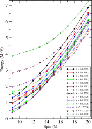
Figure 1: (Color online) The angular-momentum projected bands obtained for different intrinsic K-configuration, given in legend box, for ¹²⁸Cs nucleus.

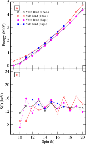
Figure 2: (Color online) Comparison of the TPSM energies after configuration mixing with the available experimental data for the yrast and side bands of the studied ¹²⁸Cs nucleus is shown in panel (a). Calculated staggering parameter $S(I)=\left[E(I)-E(I-1)\right]/2I$ is plotted along with the measured values in panel (b).

Here, $\tau$ is either $\nu$ or $\pi$, and $g_{l}$ and $g_{s}$ are the orbital and the spin gyromagnetic factors, respectively. In the calculations we use for $g_{l}$ the free values and for $g_{s}$ the free values damped by a 0.85 factor, i.e.,

$$g_{l}^{\pi}=1,~{}~{}~{}g_{l}^{\nu}=0,~{}~{}~{}g_{s}^{\pi}=5.586\times 0.85,~{}~{}~{}g_{s}^{\nu}=-3.826\times 0.85.$$ (12)

Since the configuration space is large enough to develop collectivity, we do not use core contribution. The reduced matrix element of an operator $\hat{\mathcal{O}}$ ($\hat{\mathcal{O}}$ is either $\hat{Q}$ or $\hat{\mathcal{M}}$) is expressed by

$$\,<\!\sigma_{f},I_{f}||\hat{\mathcal{O}}_{L}||\sigma_{i},I_{i}\!>\,=\sum_{\kappa_{i},\kappa_{f}}{f_{I_{i}\kappa_{i}}^{\sigma_{i}}}{f_{I_{f}\kappa_{f}}^{\sigma_{f}}}$$

$$\sum_{M_{i},M_{f},M}(-)^{I_{f}-M_{f}}\left(\begin{array}[]{ccc}I_{f}&L&I_{i}\\ -M_{f}&M&M_{i}\end{array}\right)\,<\!\phi_{\kappa_{f}}|{\hat{P}^{I_{f}}}_{K_{\kappa_{f}}M_{f}}\hat{\mathcal{O}}_{LM}\hat{P}^{I_{i}}_{K_{\kappa_{i}}M_{i}}|\phi_{\kappa_{i}}\!>\,$$ (15)

In the present study, a detailed investigation of the chiral band structures observed in ¹²⁸Cs has been performed using the TPSM approach. We have chosen this nucleus since it is the only system for which exhaustive lifetime measurements have been performed. As already discussed, the electromagnetic transition probabilities are important to probe the chiral symmetry breaking of the observed dipole bands. In Fig. 1, the projected bands, obtained from the triaxially deformed intrinsic Nilsson state by performing the three-dimensional angular-momentum projection, are displayed. Nilsson intrinsic states have been obtained with deformation parameters, $\epsilon=0.220$ and $\epsilon^{\prime}=0.14$. The axial deformation value has been adopted from particle-rotor model and other studies and the chosen value of non-axial deformation corresponds to $\gamma\sim 30^{o}$. The lowest bands

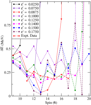
Figure 3: (Color online) Calculated energy difference ($\Delta E$) between the yrast and side bands as a function of angular-momentum for a range of the triaxial deformation $\epsilon^{\prime}$ values.

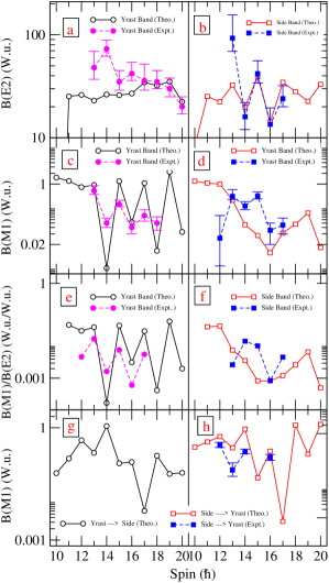
Figure 4: (Color online) Comparison of the experimental B(E2), B(M1) transition strengths and their ratio for ¹²⁸Cs [11, 12] with the calculated values for yrast and side bands are depicted in panels (a) to (f). The calculated interband transitions are shown in panels (g) and (h), and panal (h) also depicts the measured values for a few transitions.

correspond to the projected states from the intrinsic configuration with quasiparticle energy of 1.34 MeV and are obtained by specifying K-values in the three-dimensional angular-momentum projection operator, given in Eq. (6). The projected bands obtained with K=4, 5 and 7 are degenerate for I=9 and for higher spins up to I=13, K=5 and 7 are degenerate with K=4 band becoming less favoured with increasing spin. For I=14, it is noted that bands with K=1 and 2 belonging to the quasiparticle configuration of energy 1.77 MeV cross the bands belonging to the quasiparticle energy of 1.34 MeV. It is further observed that more bands belonging to the higher quasiparticle energy cross at higher spins. This crossing of the quasiparticle states has not been explored in the earlier studies of the chiral bands.

In the second stage of the calculations, projected bands obtained above are used to diagonalize the shell model Hamiltonian, Eq. (2). It is important to mention that the projected bands are not orthogonal, in general, and need to be orthogonalized before the diagonalizatoion of the Hamiltonian. The method that is adopted in the present approach, and in most of the generator coordinate methods, is to calculate the eigen-values of the norm matrix. The norm eigenvalues are non-negative quantities since the norm is a positive semi-definite matrix. However, it is quite possible that some of them may vanish. This happens under the circumstances that the multi-qp states become linearly dependent (non-orthogonal) when they are projected. Such redundant states are removed simply by discarding the zero eigenvalue solutions of the norm eigen-value equation. The details are given in the appendix of ref. [30].

Bands after diagonalization have dominant compenents from several angular-momentum projected basis configurations and the lowest two bands obtained are displayed in the top panel of Fig. 2 along with the corresponding experimental chiral bands known for ¹²⁸Cs. It is evident from Fig. 2(a) that TPSM calculations reproduce the known experimental energies of the chiral bands quite well. It is noted from the figure that the two bands are very close to each other up to I=14, and after this spin the two bands deviate with increasing spin. In Fig. 2(b), the staggering parameter, $S(I)=\left[E(I)-E(I-1)\right]/2I$ for the two calculated chiral bands are plotted and compared with the corresponding experimental numbers. It is noted that for low angular-momenta, the calculated quantity deviates considerably from the experimental values, but for higher angular-momenta a reasonable agreement is obtained. Particle-rotor model results depict a similar discrepancy at lower angular-momenta [7, 15].

To elucidate the importance of the triaxial deformation in the occurence of degenerate dipole bands, in Fig. 3 the energy difference $(\Delta E)$ between the two dipole bands is drawn as a function of the the angular-momentum for a range of the triaxial deformation values. It is evident from the figure that for lower values of $\epsilon^{\prime}$, close to the axial limit, $\Delta E$ is quite large, especially for higher angular-momentum states. However, for $\epsilon^{\prime}$ larger than 0.125, it is noted that $\Delta E$ becomes quite small for all angular-momentum states.

We now discuss the electromagnetic transition probabilities of the observed doublet bands in ¹²⁸Cs. B(E2) (from I to I-2) and B(M1) (from I to I-1) transition probabilities have been calculated using the expressions, Eqs. (9) and (10) and are shown in Fig. 4 for both the yrast and the side bands. B(E2) transition probabilities for the yrast band, displayed in Fig. 4(a), depict a slight drop at around I=13 and is due to the crossing of the quasiparticle state with energy equal to 1.77 MeV with the ground-state quasiparticle configuration. The measured B(E2) for the yrast band, displayed in Fig. 4(a), shows a more pronounced drop at a slightly higher spin value of I=15. Further, the measured B(E2) after I=16 show a smooth behaviour and is well reproduced by the TPSM calculations (see Table I). The calculated B(E2) for the side band displays a little odd-even staggering, in particular, for intermediate spin values. Except for I=13, the measured B(E2) for the few transitions are in good agreement with the calculated values and is quite evident from Table I.

The present TPSM approach provides a little improved description of the measured B(E2) values due to its microscopic treatment of the core (or vacuum) as compared to the phenomenological rotor core in 2QPTR. In TPSM, vacuum configuration (quasiparticle states) are generated by first solving triaxial Nilsson potential with the parameters $\epsilon$ and $\epsilon^{\prime}$. In the present study, we have adopted $\epsilon=0.22$, which is, as a matter of fact, same as that employed in the particle-rotor model analysis. $\epsilon^{\prime}=0.14$ has been used as this corresponds to $\gamma\sim 30^{0}$ and is important to lead to chiral configuration. In the second phase, standard BCS calculations are performed to obtain the quasiparticle states with the Nilsson basis. Although, in TPSM angular-momentum projection is performed with pairing (monopole + quadrupole) plus quadrupole-quadrupole interaction for each angular-momentum, but due to limited quasiparticle space with only one-proton and one-neutron excitations considered, it is expected that deformation of the projected states will not be very different from the vacuum or mean-field configuration. In TPSM, the vacuum configuration or mean-field is held fixed for all the projected states and this is certainly a drawback of the present analysis. In a more accurate treatment, projection after variation, mean-field is re-calculated for each angular-momentum state. We consider that due to this problem in the present approach, we observe only a marginal drop in the B(E2) in comparison to the experimental data.

Table 1: Experimental [11] and calculated intra band B(E2) transition strengths (from $I\rightarrow I-2$) for yrast and side bands of ¹²⁸Cs in $(W.u.)$

I$(\hbar)$	B(E2)		B(E2)
	Yrast Band		Side Band
	Experiment	Theory	Experiment	Theory
11		25.19		25.19
12		26.10		22.37
13	$48^{+21}_{-11}$	22.94	$93^{+63}_{-24}$	32.46
14	$73^{+16}_{-11}$	26.29	$16^{+6}_{-4}$	19.84
15	$35^{+10}_{-6}$	25.90	$42^{+14}_{-8}$	39.49
16	$42^{+12}_{-6}$	26.90	$13.5^{+6.0}_{-5.9}$	14.18
17	$36^{+16}_{-7}$	34.47		34.58
18	$35.0^{+10}_{-5}$	32.14		28.08
19	$30^{+8}_{-5}$	35.10		22.57
20	$20^{+5}_{-3}$	22.40		33.02

B(M1), shown in Fig. 4(c), for the yrast band are initially smooth, but after spin, I=13 show large odd-even staggering. For the side band, B(M1) has slightly a different behavior with B(M1) transitions showing a drop for I=13 to 16. The corresponding measured transitions are almost constant for I=13,14 and 15, and depict a drop for I=16. The phase of the odd-even staggering and the magnitudes of the B(M1) transitions are quite similar in the two dipole bands and is one of the important criterion for the chiralilty of the two bands. The calculated B(M1)/B(E2) ratios, shown in Figs. (4e) and (4f), are in good agreement with the experimental values obtained from the intensities [7]. The inter-band B(M1) transitions between yrast to side and side to yrast, shown in Figs. 4(g) and 4(h), have same phase of odd-even staggering and further are similar in magnitude. What is important is that this phase is opposite to that of the intra-band B(M1) transitions of Fig. 4(c) and 4(d) and forms another essential benchmark for the existence of the chiral geometry [6]. In Fig. 4(h), the measured B(M1) values for a few available transitions are noted to be in good agreement with the calculated values.

In conclusion, the chiral dipole band structures observed in ¹²⁸Cs have been investigated using the triaxial projected shell model for odd-odd nuclei. It has been demonstrated that observed energy levels and electromagnetic transition probabilities of the dipole bands are quite well reproduced. Furthermore, it has been demonstrated that the calculated inter band B(M1) transitions from yrast to side and vice-versa, depict opposite staggering behaviour as compared to the the in-band transitions and are in conformity with the predicted properties of the chiral bands.

The authors would like to acknowledge Dr. Ernest Grodner for providing the measured data on the electromagnetic transitions.

References

- [1] A. Bohr and B. R. Mottelson, Nuclear Structure, Vol. II (Benjamin Inc., New York, 1975).
- [2] S. G. Nilsson, Dan. Mat. Fys. Medd. 29, 16 (1955).
- [3] J. A. Sheikh and K. Hara, Phys. Rev. Lett. 82, 3968 (1999).
- [4] J. A. Sheikh, Y. Sun, and R. Palit, Phys. Lett. B 507, 115 (2001).
- [5] S. Frauendorf, J. Meng, Nucl. Phys. A 617, 131 (1997).
- [6] T. Koike, K. Starosta, and I. Hamamoto, Phys. Rev. Lett. 17, 172502 (2004).
- [7] T. Koike, K. Starosta, C. J. Chiara, D. B. Fossan, and D. R. LaFosse, Phys. Rev. C 67, 044319 (2003).
- [8] K. Starosta et al., Phys. Rev. Lett. 86, 971 (2001).
- [9] A. A. Hecht et al., Phys. Rev. C 63, 051302 (2001).
- [10] S. Zhu et al., Phys. Rev. Lett. 91, 132501 (2003).
- [11] E. Grodner et al., Phys. Rev. Lett. 97, 172501 (2006).
- [12] H. G. Ganev and S. Brant, Phys. Rev. C 82, 034328 (2010).
- [13] S. Mukhopadhyay et al., Phys. Rev. Lett. 99, 172501 (2007).
- [14] C. M. Petrache, G. B. Hagemann,I. Hamamoto and K. Starosta, Phys. Rev. Lett. 96, 112502 (2006).
- [15] S. Y.Wang, S. Q. Zhang, B. Qi, and J. Meng, Phys. Rev. C 75, 024309 (2007)
- [16] P. Olbratowski, J. Dobazewski, J. Dudek, and W. Plöciennik, Phys. Rev. Lett. 93, 052501 (2004).
- [17] V. I. Dimitrov, S. Frauendorf, and F. Donau, Phys. Rev. Lett. 84, 5732 (2000).
- [18] K. Starosta, C. J. Chiara, D. B. Fossan, T. Koike, T. T. S. Kuo, D. R. LaFosse, S. G. Rohozinski, Ch. Droste, T. Morek, and J. Srebrny, Phys. Rev. C 65, 044328 (2002).
- [19] J. Peng, J. Meng, and S. Q. Zhang, Phys. Rev. C 68, 044324 (2003).
- [20] S. Y. Wang, Y. Z. Liu, T. Komatsubara, Y. J. Ma, and Y. H. Zhang, Phys. Rev. C 74, 017302 (2006).
- [21] Y. Sun, K. Hara, J. A. Sheikh, J. G. Hirsch, V. Velazquez, and M. Guidry, Phys. Rev.C 61, 064323 (2000).
- [22] J. A. Sheikh, G. H. Bhat, Y. Sun, G. B. Vakil, and R. Palit, Phys. Rev. C 77, 034313 (2008).
- [23] J. A. Sheikh, G. H. Bhat, R. Palit, Z. Naik, and Y. Sun, Nucl. Phys. A 824, 58 (2009).
- [24] J. A. Sheikh, G. H. Bhat, Y. Sun, and R. Palit, Phys. Lett. B 688, 305 (2010).
- [25] P. Boutachkov, A. Aprahamian, Y. Sun, J. A. Sheikh, and S. Frauendorf, Eur. Phys. J. A 15, 455 (2002).
- [26] Y. Sun, J. A. Sheikh, and G.-L. Long, Phys. Lett. B 533, 253 (2002).
- [27] S. G. Nilsson, C. F. Tsang, A. Sobiczewski, Z. Szymanski, S. Wycech, C. Gustafson, I. Lamm, P. Moller and B. Nilsson, Nucl. Phys. A 131, 1 (1969).
- [28] P. Ring and P. Schuck, The Nuclear Many-Body Problem (Springer, New York, 1980).
- [29] Y. Sun and J.L. Egido, Nucl. Phys. A 580, 1 (1994).
- [30] K. Hara and Y. Sun, Int. J. Mod. Phys. E 4, 637 (1995). ͓