Alternating Superconductor–Insulator Transport Characteristics in a Quantum Vortex Chain

Abstract

Experimental studies of magnetoresistance in thin superconducting strips subject to a perpendicular magnetic field $B$ exhibit a multitude of transitions, from superconductor to insulator and vice versa alternately. Motivated by this observation, we study a theoretical model for the transport properties of a ladder–like superconducting device close to a superconductor–insulator transition. In this regime, strong quantum fluctuations dominate the dynamics of the vortex chain forming along the device. Utilizing a mapping of the vortex system at low energies to one-dimensional (1D) Fermions at a chemical potential dictated by $B$, we find that a quantum phase transition of the Ising type occurs at critical values of the vortex filling, from a superconducting phase near integer filling to an insulator near $1/2$ –filling. The current–voltage ($I-V$) characteristics of the weakly disordered device in the presence of a d.c. current bias $I$ is evaluated, and investigated as a function of $B$, $I$, the temperature $T$ and the disorder strength. In the Ohmic regime ($I/e\ll T$), the resulting magnetoresistance $R(B)$ exhibits oscillations similar to the experimental observation. More generally, we find that the $I-V$ characteristics of the system manifests a dramatically distinct behavior in the superconducting and insulating regimes.

I Introduction

In superconducting (SC) systems of reduced dimensionality (i.e., thin films and wires), transport properties are strongly affected by fluctuations in the superconducting order parameter. The most prominent manifestation of the role of fluctuations is the appearance of a finite dissipative resistance below the mean–field critical temperature $T_{c}$ of the bulk superconductor. This failure of the hallmark of superconductivity – the zero-resistance character – may persist to very low temperatures $T\ll T_{c}$, where pair breaking is negligible and the electronic state can still be described in terms of complex order parameter field representing the Bosonic degrees of freedom. In this regime, while fluctuations in the amplitude of the order parameter are suppressed, fluctuations in the phase field play a dominant role. In particular, when topological defects (vortices and phase–slips) develop dynamics, a dissipative voltage is generated in response to a current bias. In the $T\rightarrow 0$ limit, their quantum dynamics dominates and may lead to the formation of a liquid phase, characterized by a metallic or insulating behavior of the electronic system SITrev ; SIT1D .

In the one–dimensional (1D) case, i.e. in SC wires of width and thickness smaller than the coherence length $\xi$, the resistance essentially never vanishes at finite $T$ due to thermal activation of phase–slips LAMH ; TAPS (for $T\lesssim T_{c}$) or their quantum tunnelling at lower $T$ Giordano ; zaikin ; SIT1D . In contrast, in the two-dimensional (2D) case (SC films), superconductivity is well-established at sufficiently low $T$. However, by tuning an external parameter which leads to proliferation of free vortices, it is possible to drive a quantum ($T\rightarrow 0$) superconductor–insulator transition (SIT) QPT2 ; SITrev . Employing the concept of charge–flux duality Fisher , one may relate the conduction properties of the electronic system to the various phases of vortex matter by interchanging the roles of current and voltage. Thus the SC phase is associated with a vortex solid, while the insulator can be viewed as a vortex superfluid.

Experimentally, one of the most convenient ways to induce a tunable SIT in SC films is by application of a perpendicular magnetic field $B$. At fixed $T$, a positive magnetoresistance $R(B)$ is typically observed in a wide range of $B$. The SIT is then identified in the data as a crossing point of these isotherms at a critical field $B_{c}$, separating a SC phase for $B<B_{c}$ from an insulating phase for $B>B_{c}$. At finite $T$, in both phases the resistance is typically finite, and the distinction between the phases is deduced from the trend of $R$ vs. $T$: $dR/dT>0$ indicates a superconductor, and $dR/dT<0$ an insulating behavior.

Recent experimental studies of InO devices characterized by a strip geometry shahar – namely, a SC wire of width comparable to $\xi$ – offer an opportunity to probe the crossover from a 1D to 2D quantum dynamics of the topological phase–defects. The prominent observation is that in the presence of a perpendicular field $B$, the magnetoresistance $R(B)$ exhibits oscillations which amplitude is sharply increasing at low $T$, in striking resemblance to the behavior of Josephson arrays glazman and SC network systems networks . Moreover, the SIT at a high field $B_{c}$ appears to be preempted by a multitude of transitions at lower fields, from a SC to an insulator or vice versa alternately. These are indicated by multiple crossing points between different isotherms $R(B)$.

The periodicity of the above mentioned oscillations is consistent with a single flux penetration to the sample. This suggests that the observed SC or insulating behavior of the system is determined by commensuration of vortices within the strip area. In particular, when an integer number of vortices can be fitted along the strip forming a uniformly-spaced chain, superconductivity may be supported even at sufficiently high $B$ such that a large fraction of the sample area turns normal. However, deviation from commensurability of the vortex filling forces a frustrated vortex configuration, thereby weakening superconductivity. In this case, the quantum mechanical character of vortices is manifested by the formation of delocalized vortex states, facilitating their mobility across the width of the strip PGR . As a consequence, the tuning of vortex filling away from commensurability can possibly induce a quantum phase transition to a liquid state, of a metallic glazman or insulating character. This commensurate–incommensurate effect may also be manifested as magnetization plateaux, as was predicted in a theoretical study of bosonic ladders OG1 .

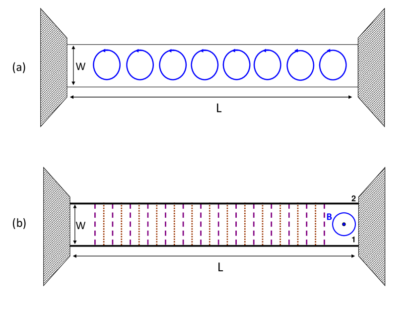
Figure 1: (color online) (a) Top view on a chain of vortices in a superconducting strip. (b) The line-junction model for the system; purple dashed lines represent the Josephson coupling $g_{J}$, and brown dotted lines the Coulomb interaction $U$ between the two SC wires.

In a recent paper AS we have studied this phenomenon within a theoretical model for a quantum vortex chain in a ladder-like SC device (see Fig. 1), which particularly addresses the strongly quantum fluctuation regime where the parameters are close to a SIT. It was shown that such system may exhibit multiple quantum phase transitions of the Ising type, manifested as SC–insulator oscillations of the Ohmic resistance $R(T,B)$. This reflects an intimate correspondence between charge-flux duality across a SIT, and the order-disorder duality characterizing the Ising transition at $1+1$-dimensions.

In this paper we present a detailed theory for the electric transport properties of the quantum vortex chain in a weakly disordered SC ladder. In particular, we derive the current–voltage ($I-V$) characteristics of the device in the presence of a d.c. current bias $I$, and investigate their behavior as a function of $B$, $I$, the temperature $T$ and the disorder strength. We find that the $I-V$ characteristics of the system manifests a dramatically distinct behavior in the SC and insulating regimes. In the Ohmic regime ($I/e\ll T$), this yields an oscillatory magnetoresistance $R(T,B)$ which exhibits $T$–dependence compatible with the experimental data.

The paper is organized as follows: in Sec. II we construct the line–junction model for the SC strip, and derive its mapping to 1D Fermions and consequently to the quantum Ising chain. In Sec. III we provide a detailed calculation of the dissipative voltage in a current–biased strip, and derive expressions for the non-linear $I-V$ characteristics and $T$–dependent magnetoresistance in the various regimes (the SC phases, insulating phases and critical regions). Our conclusions and discussion of the relation to further experiments are summarized in Sec. IV.

II The Model

We consider a thin SC strip of length $L\gg\xi$ and width $w\gtrsim\xi$, subject to a strong perpendicular magnetic field below the 2D SIT (i.e., $B\lesssim B_{c}$). A 1D chain of vortices is formed along the central axis of the strip, which can be viewed as a 1D system of particles in the presence of a self–organized effective potential dictated by the combination of vortex-vortex interaction and the boundary conditions [Fig. 1(a)]. In particular, the interface with the vacuum at the strip edges induces an effective ”image charges” potential likharev , and bulk-superconductor contacts connected to both ends of the strip enforce a fixed phase of the SC order parameter at $x=\pm L/2$. As a result, the effective potential acquires the form of a periodic 1D lattice of pinning sites separated by a uniform spacing $a=L/N$, where $N={\mathcal{I}}[BwL/\Phi_{0}]$ (with $\Phi_{0}=hc/2e$ the flux quantum, and ${\mathcal{I}}[z]$ the integer value of $z$) denotes the total number of vortices glazman . Assuming further that the high vortex density in this case leads to near merging of their cores along the central axis of the strip, the system becomes essentially equivalent to a line–junction formed by a pair of parallel SC wires separated by a normal barrier [Fig. 1(b)], subject to a magnetic field $B$ perpendicular to the junction plane.

In the low $T$ regime, pair-breaking is negligible and the properties of this system are dominated by quantum phase-fluctuations of the SC condensate. It is therefore possible to model it as a 2–leg bosonic ladder OG1 (or, equivalently, a ladder-like Josephson array glazman ), where a coordinate $x=ja$ ($j$ integer) denotes the locations of vortex cores in the continuum limit. The dynamics of the collective phase field in the wires ($\phi_{n}(x,t)$ with $n=1,2$) is governed by the effective 1D Hamiltonian

$$H_{0}=H_{1}+H_{2}+H_{int}\;,$$ (1)

in which (using units where $\hbar=1$)

$$H_{n} = \frac{1}{2}\int_{-\frac{L}{2}}^{\frac{L}{2}}dx\left[U_{0}\rho_{n}^{2}+\frac{\rho_{s}}{4m}(\partial_{x}\phi_{n})^{2}\right]\;,$$ (2)

$$H_{int} = \int_{-\frac{L}{2}}^{\frac{L}{2}}dx\left[-g_{J}\cos(\phi_{1}-\phi_{2}-qx)+U\rho_{1}\rho_{2}\right].$$ (3)

Here the operator $\rho_{n}(x)$ denotes density fluctuations of Cooper pairs in wire $n$, and can be represented as book

$$\rho_{n}(x)=-\frac{1}{\pi}\partial_{x}\theta_{n}(x)+\rho_{0}\sum_{p\not=0}e^{i2p(\pi\rho_{0}x-\theta_{n})}$$ (4)

in terms of the conjugate field $\theta_{n}(x)$ satisfying $[\phi_{n}(x),\partial_{x}\theta_{n}(x^{\prime})]=i\pi\delta(x^{\prime}-x)$. The first term in Eq. (2) hence describes a charging energy; $\rho_{s}$ is the superfluid density (per unit length) assumed to be monotonically suppressed by increasing $B$, $\rho_{0}=\rho_{s}(B=0)$ and $m$ is the electron mass. The inter–wire coupling [Eq. (3)] consists of a Josephson term and an inter–wire Coulomb interaction, of coupling strengths $g_{J}$ and $U$, respectively. Finally, the parameter

$$q=2\pi\frac{w(B-B_{N})}{\Phi_{0}}\;,\quad B_{N}=NB_{0}\,,\quad B_{0}\equiv\frac{\Phi_{0}}{wL}$$ (5)

parametrizes the deviation of the vortex density from the closest commensurate value, i.e., it denotes vortex “doping”. We note that $H_{0}$ describes an ideal system, to which we later add a disorder potential.

To further analyze the properties of this model, it is convenient to introduce symmetric and antisymmetric phase and charge fields via the canonical transformation

$$\phi_{\pm}=\frac{1}{\sqrt{2}}(\phi_{1}\pm\phi_{2}),\,\,\,\,\theta_{\pm}=\frac{1}{\sqrt{2}}(\theta_{1}\pm\theta_{2})\;.$$ (6)

In terms of these variables, the Hamiltonian (1) is separable:

$$H_{0}=H_{+}+H_{-}\\ \mathrm{where}\quad\quad\quad H_{+}=H_{LL}^{(+)}\;,\quad\quad\quad\quad H_{-}=H_{LL}^{(-)}+\int_{-\frac{L}{2}}^{\frac{L}{2}}dx\left[-g_{J}\cos(\sqrt{2}\phi_{-}-qx)+g_{c}\cos(\sqrt{8}\theta_{-})\right]\;;$$ (7)

$$H_{LL}^{(\pm)}\equiv\frac{v_{\pm}}{2\pi}\int_{-\frac{L}{2}}^{\frac{L}{2}}dx\left[K_{\pm}(\partial_{x}\theta_{\pm})^{+}\frac{1}{K_{\pm}}(\partial_{x}\phi_{\pm})^{2}\right]$$ (8)

and the parameters are given by

$$\quad K_{\pm} = \sqrt{\frac{4m(U_{0}\pm U)}{\pi^{2}\rho_{s}}}\;,\quad v_{\pm}=\sqrt{\frac{\rho_{s}(U_{0}\pm U)}{4m}}\;,$$

$$g_{c} = 2U\rho_{0}^{2}\;.$$ (9)

Here we have accounted for the most relevant interaction terms, neglecting umklapp terms included in the charging energy which are effectively suppressed due to the rapidly oscillating factor in Eq. (4). The symmetric mode (corresponding to the plasmons of total charge) governed by $H_{+}$ is therefore gapless. However, the behavior of the antisymmetric mode is dictated by the competition between two interacting (cosine) terms, and depends crucially on the value of the Luttinger parameter $K_{-}$. Below we focus on the regime of parameters close to a SIT in 1D wires, where quantum fluctuations in the phase and charge fields are maximized; i.e., $K_{-}\approx K_{c}=2$ (see Ref. zaikin, ).

We next define new canonical fields

$$\phi\equiv\frac{1}{\sqrt{2}}\phi_{-}\;,\quad\theta\equiv\sqrt{2}\theta_{-}$$ (10)

in terms of which $H_{LL}^{(-)}$ acquires the form of a Luttinger Hamiltonian with an effective Luttinger parameter $K=K_{-}/2$. For $K_{-}$ close to $K_{c}=2$, we thus obtain $K\approx 1$. This yields

$$H_{-} = \frac{v_{-}}{2\pi}\int_{-\frac{L}{2}}^{\frac{L}{2}}\left[(\partial_{x}\theta)^{2}+(\partial_{x}\phi)^{2}\right]$$

$$+ \int_{-\frac{L}{2}}^{\frac{L}{2}}dx\left[-g_{J}\cos(2\phi-qx)+g_{c}\cos(2\theta)\right]\;.$$

This model can be refermionized by introducing right ($R$) and left ($L$) moving spinless Fermion fields SNT

$$\psi_{R,L}=\frac{1}{{\sqrt{2\pi\alpha}}}e^{\pm ik_{F}x}e^{i(\mp\phi+\theta)}\;,$$ (12)

in terms of which $H_{-}$ becomes a free Hamiltonian. Here the short-distance cutoff $\alpha$ is set by the lattice constant $a$ characterizing the vortex chain, and the “Fermi momentum” $k_{F}=\pi/a+q$ is determined by the vortex filling factor [see Eq. (5)]. Quite interestingly, this implies that near a SIT, it is natural to adapt a duel representation of this system in terms of fermionic vortex fields. This stems from the approximate self-duality of $H_{-}$ (i.e., its symmetry to exchange of $\phi$ and $\theta$), implying that the natural degrees of freedom are composites of a pair charge ($2e$) and a unit of flux quantum.

The fermionic representation of $H_{-}$ is given by

$$H_{-}=\int dx\{v_{-}[\psi_{R}^{\dagger}(x)(-i\partial_{x})\psi_{R}(x)-\psi_{L}^{\dagger}(x)(-i\partial_{x})\psi_{L}(x)]\\ -\mu_{v}[\psi_{R}^{\dagger}(x)\psi_{R}(x)+\psi_{L}^{\dagger}(x)\psi_{L}(x)]\\ -J[\psi_{R}^{\dagger}(x)\psi_{L}(x)+\psi_{L}^{\dagger}(x)\psi_{R}(x)]\\ +V[\psi_{R}^{\dagger}(x)\psi_{L}^{\dagger}(x)+\psi_{L}(x)\psi_{R}(x)]\}$$ (13)

where $J=\pi\alpha g_{J}$, $V=\pi\alpha g_{c}$ and the vortex chemical potential is $\mu_{v}=\pi v_{-}q$, which vanishes at commensurate fillings. Following the analogous problem of spin-$1/2$ ladders SNT ; Tsvelik , it is useful to decompose the complex Fermions [Eq. (12)] in terms of the Majorana fields

$$\eta_{1\nu}=\frac{1}{\sqrt{2}}\left(\psi_{\nu}+\psi_{\nu}^{\dagger}\right)\;,\quad\eta_{2\nu}=\frac{1}{i\sqrt{2}}\left(\psi_{\nu}-\psi_{\nu}^{\dagger}\right)$$ (14)

($\nu=R,L$). Recasting Eq. (13) in $k$-space and using the Fourier transformed fields $\eta_{j\nu,k}=\eta_{j\nu,-k}^{\dagger}$, we obtain

$$H_{-}=\sum_{k}\Psi_{k}^{\dagger}\mathcal{H}_{k}\Psi_{k}\;,\\ \mathcal{H}_{k}\equiv\left({\begin{array}[]{*{20}c}{v_{-}k}&{i\Delta_{u}^{(0)}}&{i\mu_{v}}&0\\ {-i\Delta_{u}^{(0)}}&{-v_{-}k}&0&{-i\mu_{v}}\\ {-i\mu_{v}}&0&{v_{-}k}&{-i\Delta_{d}^{(0)}}\\ 0&{i\mu_{v}}&{i\Delta_{d}^{(0)}}&{-v_{-}k}\\ \end{array}}\right)\\ \Psi_{k}^{\dagger}\equiv\left({\begin{array}[]{*{20}c}{\eta_{1R,k}}&,&{\eta_{2L,k}}&,&{\eta_{2R,k}}&,&{\eta_{1L,k}}\end{array}}\right)\;;$$ (15)

here

$$\Delta_{u,d}^{(0)}=J\pm V$$ (16)

denote the gaps in the excitation spectrum for commensurate vortex filling ($\mu_{v}=0$), in which case $\mathcal{H}_{k}$ decouples into two independent blocks. Since $J,V$ are positive, the $u$ sector is higher in energy.

We now focus on the case of interest, where the system is assumed to be in the SC phase but close to a SIT so that the Josephson energy $J$ is slightly larger than $V$, and $\Delta_{d}^{(0)}\ll\Delta_{u}^{(0)}$. In this case, the high energy sector $u$ can be truncated, and the low-energy properties are governed by the $d$-type Fermions. Most notably, the gap $\Delta_{d}^{(0)}$ can change sign upon tuning of $J$ below the critical value $J_{c}=V$ where $\Delta_{d}^{(0)}=0$. Indeed, for $\mu_{v}=0$ each species of free massive Fermion models described by (15) can be independently mapped to an Ising chain in a transverse field Ising ; QPT2 . In particular, the low energy sector $d$ can be described by the spin Hamiltonian

$$H_{d}=-j\sum_{j}\sigma^{z}_{j}\sigma^{z}_{j+1}-V\sum_{j}\sigma^{x}_{j}$$ (17)

which possesses a quantum critical point at $J=V$.

When finite vortex “doping” is introduced by tuning $B$ away from $B_{N}$ such that $\mu_{v}\not=0$, the original $d$ and $u$ sectors mix. However, the resulting long wave-length theory can still be cast in terms of two decoupled sectors denoted $d$ (low) and $u$ (high). Moreover, the energy spectrum

$$\epsilon_{u,d}(k) = \left[J^{2}+\tilde{V}^{2}+v_{-}^{2}k^{2}\pm 2\sqrt{J^{2}\tilde{V}^{2}+(\mu_{v}v_{-})^{2}k^{2}}\right]^{1/2}\;,$$

$$\tilde{V} \equiv \sqrt{V^{2}+\mu_{v}^{2}}$$ (18)

reduces in the $k\rightarrow 0$ limit to the same form as the $\mu_{v}=0$ case:

$$\epsilon_{u,d}(k)\approx\Delta_{u,d}+\frac{1}{2}\frac{v^{2}_{u,d}k^{2}}{\Delta_{u,d}}\;,$$ (19)

with the modified velocities

$$v^{2}_{u,d}=v_{-}\left(1\pm\frac{\mu_{v}}{J\tilde{V}}\right)$$ (20)

and modified gaps given by

$$\Delta_{u,d}(B)=J\pm\tilde{V}\;.$$ (21)

The $B$-dependence of $\Delta_{u,d}$ is oscillatory due to the dependence of $\tilde{V}$ on the vortex doping $\mu_{v}$ [Eq. (18)]. While $\Delta_{u}$ remains positive and large for arbitrary $\mu_{v}$, a quantum phase transition occurs at a critical value of $\mu_{v}$ [which can be traced back to a sequence of critical fields $B_{c}^{(N)}$ via $\mu_{v}(q)$ and Eq. (5)], where $\Delta_{d}$ changes sign. As $B\rightarrow B_{c}^{(N)}$, one expects the scaling

$$|\Delta_{d}|\sim|B-B_{c}^{(N)}|\;.$$ (22)

As we show in the next Section, the above discussed Ising like quantum critical points correspond to SC–insulator transitions, marked by a dramatic change in the transport properties.

III I-V Charactaristics and Magnetoresistance

We next study the transport properties of the system in the presence of a weak scattering potential, generically induced by random, uncorrelated impurities along the coupled wires. To this end, we include a linear coupling of the density operator $\rho_{n}(x)$ [Eq. (4)] to a disorder potential $V_{D}(x)$ in the Hamiltonian. The leading contribution to dissipation arises from the backscattering term of the form book

$$H_{D}=\sum_{n=1,2}\int dx\zeta_{n}(x)\cos\{2\theta_{n}(x)\}$$ (23)

where we assume

$$\langle\zeta_{n}(x)\rangle=0\;,\quad\langle\zeta_{n}(x)\zeta_{n^{\prime}}(x^{\prime})\rangle=D\delta(x-x^{\prime})\delta_{n,n^{\prime}}.$$ (24)

Here and throughout the rest of the section, the definition of $\langle\,\rangle$ includes disorder averaging. As a result of phase-slips generated by $H_{D}$, a finite voltage will develop along the SC strip when driven by a current bias $I$.

To introduce a d.c. current bias $I$, we add a time-dependent term $It$ to the total charge operator

$$Q=-\frac{2e}{\pi}(\theta_{1}+\theta_{2}).$$

Using Eq. (6), this yields

$$\theta_{+}(x,t)=-\frac{\pi}{2\sqrt{2}e}Q(x,t)=\tilde{\theta}_{+}(x,t)-\frac{\pi}{2\sqrt{2}e}It$$ (25)

where $\tilde{\theta}_{+}(x,t)$ describes equilibrium fluctuations ($I=0$). The induced voltage along the strip is then given by $V\equiv\langle\hat{V}(L/2,t)\rangle$, where the voltage operator $\hat{V}(x,t)$ is dictated by the Josephson relation

$$\hat{V} = \frac{1}{2e}(\dot{\phi_{1}}+\dot{\phi_{2}})=\frac{1}{\sqrt{2}e}\dot{\phi}_{+}\;,$$ (26)

$$\dot{\phi}_{+} = i[H,\phi_{+}].$$

Using $H=H_{0}+H_{D}$ [Eqs. (7),(23)] we find

$$\begin{array}[]{lllllllllllllllllll}{{{\dot{\phi}}_{+}}(x,t)=\frac{{{v_{+}}{K_{+}}}}{{\sqrt{2}e}}\left\{{{\partial_{x}}{\theta_{+}}(x,t)}\right\}}&&&&&&&&&&&&&&&&&&\\ {\ -\frac{\pi}{e}\sum\limits_{n=1,2}{\int\limits_{-\frac{L}{2}}^{x}{d{x^{\prime}}{\zeta_{n}}({x^{\prime}})\sin\left[{2{\theta_{n}}({x^{\prime}},t)}\right]\,\,}}.}&&&&&&&&&&&&&&&&&&\end{array}$$ (27)

The time-evolution of $\dot{\phi}_{+}(x,t)$ can be expressed as

$$\dot{\phi}_{+}(t)=u(t)\dot{\widetilde{\phi}}_{+}(t)u^{\dagger}(t),$$ (28)

where $\dot{\widetilde{\phi}}_{+}(t)$ is the operator in the interaction representation

$$\dot{\widetilde{\phi}}_{+}(t)=e^{iH_{0}t}\dot{\phi}_{+}e^{-iH_{0}t}\;,$$ (29)

and

$$u(t)\equiv e^{i(H_{0}+H_{D})t}e^{-iH_{0}t}.$$ (30)

Assuming a weak disorder which allows a perturbative treatment of $H_{D}$, $u(t)$ is given to first order by

$$u(t)=1+{\underset{-\infty}{i\int}^{t}}dt^{\prime}H_{D}(t^{\prime}).$$ (31)

Substituting Eq. (31) in Eq. (28), one obtains

$$\langle\dot{\phi_{+}}(x,t)\rangle=i{\overset{t}{\underset{-\infty}{\int}}dt^{\prime}\left\langle\left[H_{D}(t^{\prime}),\dot{\widetilde{\phi}}_{+}(x,t)\right]\right\rangle}.$$ (32)

Using Eqs. (23), (26) and (32), and recalling Eq. (6), we obtain an expression for the d.c. voltage

$$V=V_{1}+V_{2}$$ (33)

where

$$V_{1(2)}\equiv\frac{iDL\pi}{e}\int^{t}_{-\infty}dt^{\prime}\left\langle\left[\sin\left(\sqrt{2}\{\theta_{+}(t)\pm\theta_{-}(t)\}\right)\cos\left(\sqrt{2}\{\theta_{+}(t^{\prime})\pm\theta_{-}(t^{\prime})\}\right)\right]\right\rangle$$ (34)

(here $\theta_{\pm}(t)\equiv\theta_{\pm}(0,t)$). Introducing the operators

$$A_{1(2)}(x,t)\equiv e^{i\sqrt{2}(\tilde{\theta}_{+}(x,t)\pm\theta_{-}(x,t))}$$ (35)

where $\tilde{\theta}_{+}$ is defined in Eq. (25), we obtain the voltage-current characteristic

$$V(I)=\frac{{DL\pi}}{{4e}}\sum_{n=1,2}\int_{-\infty}^{\infty}d{t^{\prime}}i\Theta(t-{t^{\prime}})\left\{{e^{i\frac{{\pi I}}{{2e}}({t^{\prime}}-t)}}\left\langle{\left[{{A_{n}}(t),A_{n}^{\dagger}({t^{\prime}})}\right]}\right\rangle-{e^{-i\frac{{\pi I}}{{2e}}({t^{\prime}}-t)}}\left\langle{\left[{A_{n}^{\dagger}(t),{A_{n}}({t^{\prime}})}\right]}\right\rangle\right\}\;.$$ (36)

In terms of the retarded Green’s functions

$$\begin{array}[]{ll}\chi^{(n)}_{ret}(t)&=-i\Theta(t)\left\langle\left[A_{n}(t),A^{\dagger}_{n}(0)\right]\right\rangle\\ &=-2\Theta(t)\Im m\{\chi_{n}(t)\}\end{array}$$ (37)

with

$$\chi_{n}(t)\equiv\langle A_{n}(t)A^{\dagger}_{n}(0)\rangle,$$ (38)

we finally obtain

$$\begin{array}[]{ll}V(I)&=\frac{DL\pi}{2e}\sum\limits_{n=1,2}\overset{\infty}{\underset{0}{\int}}dt\sin\left(\frac{\pi It}{2e}\right)\Im m\{{\chi_{n}(t)}\}\\ &=\frac{DL\pi}{4e}\sum\limits_{n=1,2}\overset{\infty}{\underset{-\infty}{\int}}dt\sin(\frac{\pi It}{2e})\chi_{n}(t)\end{array}$$ (39)

where in the last step we have used the fact that $\Im m\{\chi_{n}(t)\}$ is the antisymmetric part of $\chi_{n}(t)$ under $t\shortrightarrow-t$. This correlation function can be evaluated utilizing the low-energy theory developed in Sec. II.

To leading order in the perturbation $H_{D}$, the expectation value $\langle\,\rangle$ may be replaced by $\langle\,\rangle_{0}$, evaluated with respect to $H_{0}$. Since the ${\theta_{+}}$, $\theta_{-}$ degrees of freedom are decoupled in $H_{0}$, the correlation function

$$\chi_{1}=\chi_{2}\equiv\chi$$ (40)

where

$$\chi(t)=\left\langle e^{i\sqrt{2}(\tilde{\theta}_{+}(x,t)+\theta_{-}(x,t))}e^{-i\sqrt{2}(\tilde{\theta}_{+}(0,0)+\theta_{-}(0,0))}\right\rangle_{0}$$ (41)

decouples into

$$\chi(t) = \chi_{C+}(t)\chi_{C-}(t)+\chi_{S+}(t)\chi_{S-}(t)+\chi_{S+}(t)\chi_{C-}(t)+\chi_{C+}(t)\chi_{S-}(t)$$ (42)

$$\chi_{C\pm} \equiv \langle\cos\{\sqrt{2}\theta_{\pm}(t)\}\cos\{\sqrt{2}\theta_{\pm}(0)\}\rangle_{\pm}\;,\quad\quad\chi_{S\pm}\equiv\langle\sin\{\sqrt{2}\theta_{\pm}(t)\}\sin\{\sqrt{2}\theta_{\pm}(0)\}\rangle_{\pm}\;.$$ (43)

Here $\langle\,\rangle_{\pm}$ are evaluated with respect to $H_{\pm}$. The symmetric mode described by $H_{+}$ is a Luttinger liquid [see Eq. (7)], hence book

$$\chi_{C+}(t)=\chi_{S+}(t)=\lim_{\epsilon\rightarrow 0}\left(\frac{-(\pi\alpha T/v_{+})}{\sinh\{\pi T\left(t-i\epsilon\right)\}}\right)^{\frac{1}{K_{+}}}.$$ (44)

In contrast, as discussed below, the correlations characterizing the antisymmetric mode [$\chi_{C-}(t)$ and $\chi_{S-}(t)$] depend crucially on the parameters of (15), and in particular on the magnitude and sign of the masses $\Delta_{u,d}$.

To evaluate $\chi_{C-}$ and $\chi_{S-}$, we first note that in terms of the field $\theta$ [Eq. (10)], they correspond to correlation functions of $\cos\theta$, $\sin\theta$, which lack a local representation in terms of Fermion fields. However, a convenient expression is available in terms of the two species of order ($\sigma_{u,d}$) and disorder ($\tilde{\sigma}_{u,d}$) Ising fields SNT ; Ising : for $\Delta_{d}>0$,

$$\cos\theta\sim\sigma_{u}\tilde{\sigma}_{d}\;,\quad\sin\theta\sim\tilde{\sigma}_{u}\sigma_{d}\;.$$ (45)

For $\Delta_{d}<0$, the roles of $\sigma_{d}$, $\tilde{\sigma}_{d}$ are simply interchanged. The correlators $\chi_{C-}$, $\chi_{S-}$ can therefore be expressed in terms of $C_{\lambda}(t)=\langle\sigma_{\lambda}(t)\sigma_{\lambda}(0)\rangle$, $\tilde{C}_{\lambda}(t)=\langle\tilde{\sigma}_{\lambda}(t)\tilde{\sigma}_{\lambda}(0)\rangle\,$ ($\lambda=u,d$), which have known analytic approximations in the semi–classical regime ($|\Delta_{\lambda}|\gg T$) SNT ; sachdev ; BMASR :

$$C_{\lambda}(t)\sim|\Delta_{\lambda}|^{1/4}K_{0}(i|\Delta_{\lambda}|t),\quad\tilde{C}_{\lambda}(t)\sim|\Delta_{\lambda}|^{1/4}$$ (46)

[with $K_{0}(z)$ the modified Bessel function]. In the quantum critical regime ($|\Delta_{d}|\ll T$), $C_{d}(t)\sim\tilde{C}_{d}(t)\sim t^{-1/4}$.

Employing Eqs. (44), (46), it is possible to evaluate the retarded correlation function and thus $V(I)$ in either side of the quantum critical point of the Ising model $d$. Below we show that the resulting dramatically distinct behavior of the dissipative transport in the disordered and ordered phases of the Ising system identifies them as “superconducting” and “insulating”, respectively.

III.1 Superconducting phases

We first derive expressions for the $I-V$ characteristics near commensurate fields $B_{N}$ [Eq. (5)] where $\Delta_{d}\sim\Delta_{d}^{(0)}>0$, in the low $T$ regime where Eq. (46) holds. Neglecting terms of order $e^{-\Delta_{u}/T}$ and keeping the first order in $D$, we obtain form Eq. (39)

$$V^{(1)}(I)=C\int^{\infty}_{-\infty}dt\sin\left(\frac{\pi It}{2e}\right)\left(\frac{-\left(\pi\alpha T/v_{+}\right)}{\sinh(\pi T(t-i\varepsilon))}\right)^{\frac{1}{K_{+}}}K_{0}(i\Delta_{d}t)\;,\quad{\rm where}\quad C\propto DL|\Delta_{u}\Delta_{d}|^{1/4}.$$ (47)

For $\frac{\pi I}{2e}<\Delta_{d}$, this yields a non-linear $I-V$ curve

$$\begin{array}[]{l}V^{(1)}(I)\approx V_{s}^{(1)}\sqrt{\frac{T}{\Delta_{d}(B)}}e^{-\Delta_{d}(B)/T}\sinh\left(\frac{\pi I}{2eT}\right)\;,\\ V_{s}^{(1)}\propto D[\Delta_{d}(B)]^{K_{+}^{-1}(B)+\frac{1}{4}}\end{array}$$ (48)

which exhibits a threshold at a critical current $I_{c}=\frac{2e\Delta_{d}}{\pi}$ in the limit $T\rightarrow 0$. In the Ohmic regime $I/e\ll T$, one obtains a contribution to the magnetoresistance of the form

$$\begin{array}[]{lll}R^{(1)}(T,B)\approx R_{s}\sqrt{\frac{\Delta_{d}(B)}{T}}e^{-\Delta_{d}(B)/T}\;,\\ R_{s}\propto D\left(\Delta_{d}(B)\right)^{K_{+}^{-1}(B)-\frac{3}{4}}\;.\end{array}$$ (49)

Superimposed on a moderate monotonic increase with $B$ arising from $K_{+}(B)$ due to the suppression of $\rho_{s}$ [Eq. (9)], the exponential factor leads to a strong decrease and $R^{(1)}\rightarrow 0$ at $T\rightarrow 0$ as long as $\Delta_{d}(B)>0$ is finite. The disordered Ising phase is thus identified as superconducting: it corresponds to a state where the phase of the SC order-parameter in the two wires is locked. This suggests that the fields $\sigma_{d}$ physically represent phase-slips in the antisymmetric sector (which are gapped in this regime).

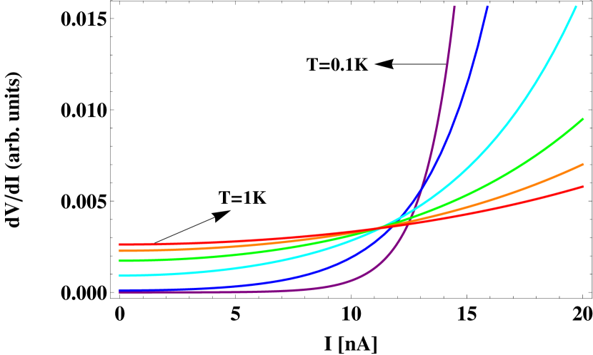
Figure 2: (color online) Differential resistance vs. current bias in the superconducting phase for temperatures $T=0.1$K, $0.2$K, $0.4$K, $0.6$K, $0.8$K and $1.0$K, for a fixed $B$ such that $\Delta_{d}=1.0$K and $K_{+}=2.1$ (see text); the disorder parameter is chosen such that $Da^{3}/v_{-}^{2}=0.1$.

The above analysis indicates that the first order in $D$ yields an exponentially small voltage for $I,T\rightarrow 0$, suggesting that one should examine the perturbation scheme in $H_{D}$ [Eq. (23)] more carefully OG2 . Indeed, if we evaluate the expectation value $\langle\,\rangle$ expanding to the next order in $D$, we find that the correlation functions $\chi_{n}$ acquire corrections to Eq. (41) of the form

$$\delta\chi\propto D\langle e^{\pm i2\theta_{1}(t)}e^{\pm i2\theta_{2}(t)}e^{\mp i2\theta_{1}(0)}e^{\mp i2\theta_{2}(0)}\rangle_{0}\;.$$ (50)

Using Eq.(6), this can be written as

$$\delta\chi\propto D\langle e^{i2\sqrt{2}\theta_{+}(t)}e^{-i2\sqrt{2}\theta_{+}(0)}\rangle_{0}\;.$$ (51)

The resulting contribution to the voltage

$$V^{(2)}(I)\approx\frac{DL\pi}{4e}\overset{\infty}{\underset{-\infty}{\int}}dt\sin\left(\frac{\pi It}{2e}\right)\delta\chi(t)$$ (52)

is associated with scattering processes which do not involve the antisymmetric mode, and hence are not affected by the superconducting order. These correspond to coincidental events incorporating two scatterers located on two different wires simultaneously, and therefore their probability is of the order of $D^{2}$. The gapless symmetric mode experiences backscattering in such events, similarly to the usual plasmon mode in a strictly 1D SC wire. Inserting the Luttinger liquid correlation function

$$\delta\chi(t)\sim D\left(\frac{-(\pi\alpha T/v_{+})}{\sinh\{\pi T\left(t-i\epsilon\right)\}}\right)^{\frac{4}{K_{+}}}\;,$$ (53)

we obtain GRbook

$$V^{(2)}(I)=V^{(2)}_{s}\left\{B\left(-\frac{iI}{4eT}+\frac{2}{K_{+}},1-\frac{4}{K_{+}}\right)-B\left(\frac{iI}{4eT}+\frac{2}{K_{+}},1-\frac{4}{K_{+}}\right)\right\}\quad{\rm where}\quad V_{s}^{(2)}\propto D^{2}$$ (54)

and $B(x,y)=\frac{\Gamma(x)\Gamma(y)}{\Gamma(x+y)}$ is the Beta function.

The full $I-V$ characteristic in the SC phases ($\Delta_{d}(B)>T,I/e$) can finally be expressed as

$$V(I)=V^{(1)}(I)+V^{(2)}(I)\;,$$ (55)

where $V^{(1)}(I)$, $V^{(2)}(I)$ represent contributions from odd and even orders in the disorder parameter $D$ respectively, and can be viewed as two resistors connected in series. To leading order in $D$, they are given by Eqs. (48) and (54), yielding the $I,T$-dependence depicted in Fig. 2. Note that although the second term is higher order in the scattering rate $D$, it becomes the dominant contribution in the limits $T,I\rightarrow 0$ as the first term is exponentially suppressed. For $I/e\gg T$, this indicates a power-law $I-V$ relation

$$V(I)\sim D^{2}I^{\kappa(B)+1}\;,\quad\kappa(B)\equiv\frac{4}{K_{+}(B)}-2$$ (56)

and in the Ohmic regime ($I/e\ll T$)

$$R(T,B)\sim D^{2}T^{\kappa(B)}\;.$$ (57)

By definition of the Luttinger parameters $K_{\pm}$ [Eq. (9)], $K_{+}\gtrsim K_{-}$ and hence the assumption $K_{-}=2$ implies $K_{+}\gtrsim 2$. As a consequence, the exponent $\kappa(B)$ [Eq. (56)] is small and slightly negative. We therefore conclude that in spite of the phase–locking ordering of the antisymmetric phase mode, the true $T,I\rightarrow 0$ behavior of the electric transport exhibits an insulating behavior. In practice, however, the insulating character may be manifested only at extremely low $T$. At moderately low $T$, the sub-leading term $V^{(1)}(I)$ is expected to be appreciable, and indicate a threshold at a critical current $I_{c}$, directly related to an activation gap in the Ohmic resistance [Eq. (49)]:

$$\log\,R\sim\Delta_{d}=\frac{\pi I_{c}}{2e}\;.$$ (58)

The oscillatory nature of $\Delta_{d}(B)$ as $B$ is tuned through commensurate and incommensurate values should be reflected in the $B$-dependence of $I_{c}$, which is maximized at commensurate values $B_{N}$ and vanishes in the vicinity of incommensurate regimes $B\sim B_{N+\frac{1}{2}}$.

III.2 Insulating phases

We next consider the insulating phase, realized in the vicinity of incommensurate fields $B\sim B_{N+\frac{1}{2}}$ such that $\Delta_{d}<0$. In this case, both species of Ising models $u$ and $d$ are in the ordered phase, and for $T\ll|\Delta_{d}|$ the correlation function characterizing the antisymmetric mode is given up to exponentially small corrections by a constant

$$\chi_{-}(t)\sim|\Delta_{u}\Delta_{d}|^{1/4}\;.$$ (59)

As a result, $\chi(t)=\chi_{+}(t)\chi_{-}(t)$ [Eq. (41)] is dominated by the Luttinger liquid correlations [Eq. (44)] characterizing the symmetric mode. Keeping the leading order in $D$ in Eq.(39), we thus find an expression for the $I-V$ characteristics of the form

$$\begin{array}[]{l}V(I)=V_{i}\left\{B\left(-\frac{iI}{4eT}+\frac{1}{2K_{+}},1-\frac{1}{K_{+}}\right)-B\left(\frac{iI}{4eT}+\frac{1}{2K_{+}},1-\frac{1}{K_{+}}\right)\right\}\;,\quad{\rm where}\quad V_{i}\propto D|\Delta_{u}\Delta_{d}|^{1/4}\;.\end{array}$$ (60)

Typical plots of the resulting dynamic resistance $dV/dI$ vs. $I$ are depicted in Fig. 3, indicating a zero-bias peak at $I\rightarrow 0$, in sharp distinction from the SC phase (Fig. 1). For $I/e\gg T$, we obtain a diverging power-law

$$V(I)\sim DI^{1-\gamma(B)}\;,\quad\gamma(B)\equiv 2-\frac{1}{K_{+}(B)}$$ (61)

and in the Ohmic regime ($\frac{I}{e}\ll T$)

$$R(T,B)\sim DT^{-\gamma(B)}\;.$$ (62)

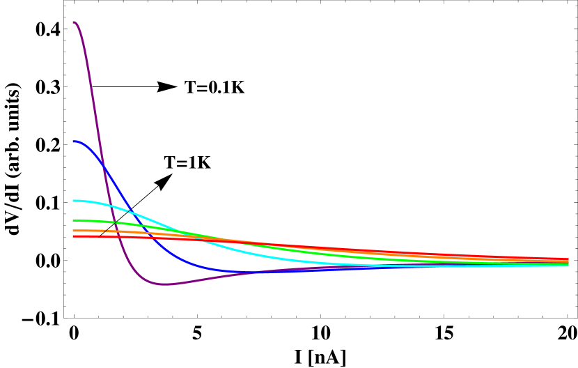
Figure 3: (color online) Differential resistance vs. current bias in the insulating phase for temperatures $T=0.1$K, $0.2$K, $0.4$K, $0.6$K, $0.8$K and $1.0$K, for a fixed $B$ such that $|\Delta_{d}|=1.0$K and $K_{+}=2.1$ (see text); the disorder parameter is chosen such that $Da^{3}/v_{-}^{2}=0.1$.

Compared to the power-law contributions to dissipation in the SC phase [Eqs. (56) and (57)], these results indicate a stronger divergence at low $T$ and $I$. This behavior stems from the fact that the antisymmetric mode is in the insulating, charge-ordered phase, and consequently backscattering processes by a single impurity are favored. Moreover, since $K_{+}^{-1}\lesssim\frac{1}{2}$, the exponent $\gamma(B)>3/2$ indicating that the disorder potential is highly relevant. In the truly $T,I\rightarrow 0$ limit (i.e., below a crossover temperature scale $T_{loc}$ which depends on the disorder strength $D$), the perturbative treatment of $H_{D}$ leading to Eq. (60) is not valid and localization takes over, yielding an exponentially diverging resistance book . We note that at moderately low $T$ and $I$, Eq. (60) is still valid and appears to be compatible with the experimental data shahar .

III.3 Critical regime

The above analysis implies that the quantum critical points at $B_{c}^{(N)}$ (where $\Delta_{d}=0$) correspond to SC-I and I-SC transitions alternately, associated with the change of ordering in the antisymmetric mode from phase-ordered to charge-ordered ground state. These transitions are marked by a dramatic qualitative change in the shape of the non-linear $I-V$ curves, and in the $T$-dependence of the Ohmic resistance, as $B$ crosses $B_{c}^{(N)}$. However, note that unlike the 2D SIT, the quantum critical points can not be easily identified in the transport properties, e.g. as crossing points of isotherms where $R(B,T)$ exhibits a metallic behavior. In the critical regime ($T\gg|\Delta_{d}|$), the antisymmetric mode is characterized by power-law correlations $\chi_{-}(t)\sim t^{-1/4}$ and consequently

$$R(T,B)\sim T^{\frac{1}{4}-\gamma(B)}\;.$$ (63)

This reflects once again an insulating behavior, characteristic to the 1D nature of the system. It stems from the presence of a gapless mode (the symmetric plasmon), which is not immune to backscattering processes.

IV Discussion

In this study, we have shown that the low-$T$ transport properties of a ladder–like superconducting device subject to a perpendicular magnetic field may signify a multitude of quantum phase transitions from a SC to insulating phases alternately, when its parameters are tuned close to the 2D SIT. These transitions stem from the quantum mechanical nature of the vortex chain accommodated along the central axis of the device, and reflect the competition between a Josephson coupling and a charging energy between the SC edges of the device, which govern the antisymmetric phase–charge mode. The former dominates near commensurate values of the vortex density, and the latter near incommensurate ($1/2$-integer) densities. The quantum critical points are of the Ising type: this is a manifestation of the $Z_{2}$ symmetry characterizing the antisymmetric mode, associated with interchanging the two legs of the ladder.

The analysis presented in Sec. III indicates, however, that the electric transport properties are complicated by the presence of a gapless symmetric phase–charge mode, which provides a dissipative environment. As a result, the voltage response to a current bias does not exhibit a strictly superconducting behavior even in the phases classified as SC. Nevertheless, for weakly disordered systems it is possible to observe a clear signature of the SC nature of these phases at finite $T$ and $I$. Subtracting the contribution of backscattering exclusive to the symmetric mode, which can be viewed as a resistor connected in series, one obtains an activated behavior of the $I-V$ curve and the $T$-dependent resistance [see Fig. 1 and Eq. (58)]. This behavior is sharply distinct from the insulating phases, where the differential resistance $dV/dI$ exhibit a zero-bias anomaly peak [see Fig. 2]. Moreover, in principle it is possible to detect the quantum critical points ($B_{c}^{(N)}$) separating the two phases by probing the $B$-dependence of the activated gap [Eq. (58)].

It should be noted that the analysis thus far relies on some crucial simplifying assumptions. In particular, it has been assumed that the model for the antisymmetric mode is tuned to a self-dual point, where $K_{-}=2$. In this special point, where both the phase and charge fields are not well-defined, the chain of vortices is exactly describable in terms of free Fermions. The question arises, to what extent our results are robust against a finite detuning away from the self-dual point, i.e. when $K_{-}=2+\delta K$. Such corrections induce interactions among the Fermions. However, since in both the SC and insulating phases the Fermions are massive and excitations are gapped, these interactions can be treated perturbatively as long as $(v_{-}/a)\delta K\ll|\Delta_{d}|$. This approximation fails when $|\Delta_{d}|\rightarrow 0$ and the critical point is shifted, but the Ising-type nature of the transition is maintained SAR . The phenomenology manifested by the transport properties as discussed above would therefore be essentially the same.

Another point of concern when adapting the model to describe a realistic system is the role of finite size effects. In Sec. III, the correlation functions were evaluated for finite $T$ assuming that the length of the system $L\rightarrow\infty$. However, we note that the SC nanowires studied, e.g., in Ref. shahar, , typically have a finite length of the order of a few microns. This introduces an additional low-energy cutoff $T_{L}\equiv v_{-}/L$. Using typical values of the plasma velocity for $v_{-}$ (see, e.g., Ref. zaikin, ), we estimate $T_{L}\sim 1$K. This implies that for sub-Kelvin temperatures, $T_{L}$ effectively replaces $T$ as the low-energy cutoff. In the SC phases, the activated contribution to the resistance is therefore expected to be $\sim e^{-\Delta_{d}/T_{L}}$. Noting that $T_{L}$ is also associated with the zero-point energy of phase-fluctuations, this represents contribution due to macroscopic quantum tunneling of vortices out of a metastable state in the finite-size SC device LegCal .

Finally, we wish to point out that a ladder–like SC device where the parameters are conveniently tunable (e.g., a Josephson ladder) can serve as an interesting playground for the study of emergent fractional degrees of freedom. In particular, when the gap $\Delta_{d}$ vanishes, the eigenstates of Eq. (15) (at zero energy) become Majorana Fermions. Therefore, as recently proposed by Tsvelik Majorana , inhomogeneous SC devices can be potentially utilized to realize localized Majorana modes at interfaces between superconducting and insulating segments.

- (1) For a review and extensive references, see A. F. Hebard, in Strongly Correlated Electronic Materials (The Los Alamos Symposium 1993), Eds. K. S. Bedell, Z. Wang, D. E. Meltzer, A. V. Balatsky and E. Abrahams, Addison Wesley (1994), p. 251; G. T. Zimanyi, ibid p. 285; Y. Liu and A. M. Goldman, Mod. Phys. Lett. B 8, 277 (1994); S. L. Sondhi, S. M. Girvin, J. P. Carini and D. Shahar, Rev. Mod. Phys. 69, 315 (1997) A. M. Goldman and N. Markovic, Physics Today 51, 39 (1998).
- (2) K.Yu.Arutyunov, D. S. Golubev and A. D. Zaikin, Physics Reports 464, 1 (2008), and refs. therein.
- (3) J. S. Langer and V. Ambegaokar, Phys. Rev. 164, 498 (1967); D. E. McCumber and B. I. Halperin, Phys. Rev. B 1, 1054 (1970).
- (4) See, e.g., R. S. Newbower, M. R. Beasley and M. Tinkham, Phys. Rev. B 5, 864 (1972).
- (5) N. Giordano, Phys. Rev. Lett. 61, 2137 (1988); N. Giordano, Phys. Rev. B 41, 6350 (1990).
- (6) A. D. Zaikin, D. S. Golubev, A. van Otterlo and G. T. Zimanyi, Phys. Rev. Lett. 78, 1552 (1997).
- (7) S. Sachdev, Quantum Phase Transitions (Cambridge University Press (1999)).
- (8) M. P. A. Fisher, Phys. Rev. Lett. 65, 923 (1990).
- (9) A. Johansson, G. Sambandamurthy, N. Jacobson, D. Shahar, and R. Tenne, Phys. Rev. Lett. 95, 116805 (2005); A. Johansson, G. Sambandamurthy and D. Shahar, unpublished.
- (10) C. Bruder, L.I. Glazman, A.I. Larkin, J.E. Mooij and A. van Oudenaarden, Phys. Rev. B 59, 1383 (1999).
- (11) M. D. Stewart Jr., A. Yin, J. M. Xu and J. M. Valles Jr., Phys. Rev. B 77, 140501(R) (2008); I. Sochnikov, A. Shaulov, Y. Yeshurun, G. Logvenov and I. Bozovic, Nature Nanotechnology 5, 516 (2010).
- (12) D. Pekker, G. Refael and P. Goldbart, Phys. Rev. Lett. 107, 017002 (2011).
- (13) E. Orignac and T. Giamarchi, Phys. Rev. B 64, 144515 (2001).
- (14) Y. Atzmon and E. Shimshoni, Phys. Rev. B 83, 220518(R) (2011).
- (15) K. K. Likharev, Sov. Phys. JETP 34, 906 (1972).
- (16) T. Giamarchi, Quantum Physics in One Dimension, (Oxford, New York, 2004).
- (17) D. G. Shelton, A. A. Nersesyan and A. M. Tsvelik, Phys. Rev. B 53, 8521 (1996).
- (18) A. M. Tsvelik, Phys. Rev. B 83, 104405 (2011).
- (19) A. O. Gogolin, A. A. Nersesyan and A. M. Tsvelik, Bosonization and Strongly Correlated Systems (Cambridge University Press, 1998).
- (20) S. Sachdev and A. P. Young, Phys. Rev. Lett. 78, 2220 (1997).
- (21) Decoupling of the and sectors is justified by the significant difference in their masses (); see E. Boulat, P. Mehta, N. Andrei, E. Shimshoni and A. Rosch, Phys. Rev. B 76, 214411 (2007).
- (22) E. Orignac and T. Giamarchi, Phys. Rev. B 57, 11713 (1998).
- (23) I. S. Gradshteyn and I. M. Ryzhik, Tables of Integrals, Series and Products (Academic Press, 1980).
- (24) A. O. Caldeira and A. J. Leggett, Ann. Phys. 149, 374 (1983), and references therein.
- (25) E. Sela, A. Altland and A. Rosch, Phys. Rev. B 84, 085114 (2011).
- (26) A. M. Tsvelik, arXiv:1106.2996.