The VAST Survey – II. Orbital motion monitoring of A-type star multiples

Abstract

As a part of our ongoing Volume-limited A-Star (VAST) adaptive optics survey, we have obtained observations of 26 binary systems with projected separations $<$100 AU, 13 of which have sufficient historical measurements to allow for refinement of their orbital elements. For each system with an estimated orbit, the dynamical system mass obtained was compared with the system mass estimated from mass-magnitude relations. Discrepancies between the dynamical and theoretical system mass can be explained by the presence of a previously unresolved spectroscopic component, or by a non-solar metallicity of the system. Using this approach to infer the presence of additional companions, a lower limit to the fraction of binaries, triples, and quadruples can be estimated as 39, 46, and 15 per cent, for systems with at least one companion within 100 AU. The fraction of multiple systems with three or more components shows a relative increase compared to the fraction for Solar-type primaries resolved in previous volume-limited surveys. The observations have also revealed a pair of potentially young ($<$100 Myr) M-dwarf companions, which would make an ideal benchmark for the theoretical models during the pre-Main Sequence contraction phase for M-dwarfs. In addition to those systems with orbit fits, we report 13 systems for which further orbital monitoring observations are required, 11 of which are newly resolved as a part of the VAST survey.

1 Introduction

The orbits of binary stars offer one of the few techniques to determine stellar masses, or masses and radii in cases with a favorable geometry (e.g. Andersen et al., 1991). Orbits of binaries with young ages are particularly important to test theoretical evolutionary models, and examples include a double-lined eclipsing binary in Orion (e.g.Stassun et al., 2008). Low mass stars and brown dwarfs also represent a regime requiring empirical calibration, and the visual orbits of nearby M-, L-, and T- dwarfs have been used to measure system masses and compare with theoretical mass-luminosity relations (Dupuy et al., 2009).

Visual orbits also provide a method to search for evidence of additional components and determine higher order multiplicity, by identifying systems with dynamical masses significantly in excess of the theoretical predictions. These visual binaries with an indication of unresolved companions can be monitored with spectroscopy or interferometry to determine the properties such as period and mass ratio of the closer pair and augment the statistics compiled from catalogues (Tokovinin, 2008). The properties of higher order multiple systems represent tests of formation scenarios including fragmentation of cores (e.g. Pringle, 1989; Bonnell, 2001) and disks (e.g. Stamatellos et al., 2007; Kratter et al., 2010) and may be influenced by processes such as accretion (e.g. Bate, 2000) and dynamical interactions (e.g. McDonald & Clarke, 1995; Lodato et al., 2007)

In this paper, a subset of the systems resolved by our ongoing volume-limited A-star (VAST) survey are used to determine dynamical system masses from orbit fits and to compare the results with theoretical models and search for additional unresolved stellar companions. The sample of AO-imaged binaries considered in this study is detailed in Section 2, and a short summary of the new observations is given in Section 3. The data analysis, including the AO image processing to determine the relative positions and the subsequent orbit determination from the compilation of position data, is explained in Section 4. Section 5 reports the astrometric results from the new measurements and the orbital elements and masses based on the orbit fits. The discussion in Section 6 covers a comparison with theoretical mass-magnitude relations, an assessment of the higher order multiplicity, and the identification of a set of targets for continued monitoring. Finally, Section 7 provides a summary and future directions for the project.

2 Sample

Table 1: Basic properties of sample members

HIP	Name	HR	HD	ADS	Spectral	Distance		$V_{\rm T}$		$K_{\rm s}$
					Type	(pc)		(mag)		(mag)
Orbit Subsample
5300	$\upsilon$ Phe	331	6767		A3IV	57.0$\pm$	2.0	5.230$\pm$	0.001	4.78$\pm$	0.02
9480	48 Cas	575	12111	1598	A3IV	35.3$\pm$	0.6	4.533$\pm$	0.002	4.08$\pm$	0.13a
11569	$\iota$ Cas	707	15089	1860	A5p	40.7$\pm$	1.3	4.496$\pm$	0.003	4.25$\pm$	0.03
17954		1188	23985	2799	A2V+…	56.5$\pm$	1.8	5.259$\pm$	0.004	4.81$\pm$	0.02
28614	$\mu$ Ori	2124	40932	4617		47.5$\pm$	1.5	4.150$\pm$	0.002	3.64$\pm$	0.26
36850	Castor	2891/2890	60178J	6175	A2Vm	15.6$\pm$	0.9	1.590$\pm$	0.020	1.47$\pm$	0.03a
44127	$\iota$ UMa	3569	76644		A7V	14.51$\pm$	0.03	3.159$\pm$	0.002	2.67$\pm$	0.03b
47479		3863	84121		A3IV	72.6$\pm$	2.2	5.334$\pm$	0.003	4.80$\pm$	0.02
76952	$\gamma$ CrB	5849	140436	9757	B9IV+…	44.8$\pm$	1.0	3.819$\pm$	0.002	3.67$\pm$	0.23
77660	b Ser	5895	141851		A3Vn	49.8$\pm$	0.8	5.112$\pm$	0.002	4.70$\pm$	0.02
80628	$\upsilon$ Oph	6129	148367		A3m	41.0$\pm$	1.5	4.657$\pm$	0.003	4.17$\pm$	0.04
82321	52 Her	6254	152107	10227	A2Vspe…	55.3$\pm$	1.0	4.833$\pm$	0.003	4.57$\pm$	0.02
93506	$\zeta$ Sgr	7194	176687	11950	A2.5Va	27.0$\pm$	0.6	2.617$\pm$	0.003	2.29$\pm$	0.23
Monitoring Subsample
128			224890		Am…	70.8$\pm$	1.7	6.521$\pm$	0.004	6.02$\pm$	0.02
2381		118	2696		A3V	53.1$\pm$	0.8	5.188$\pm$	0.003	4.83$\pm$	0.02
2852	BG Cet	151	3326		A5m…	48.9$\pm$	0.8	6.093$\pm$	0.004	5.42$\pm$	0.01
5310	79 Psc	328	6695		A3V	47.3$\pm$	1.7	5.581$\pm$	0.003	5.22$\pm$	0.02
18217		1192	24141		A5m	50.5$\pm$	1.1	5.806$\pm$	0.004	5.37$\pm$	0.02
29852		2265	43940		A2V	61.9$\pm$	1.0	5.895$\pm$	0.003	5.44$\pm$	0.02
51384		4062	89571		F0IV	40.6$\pm$	0.6	5.549$\pm$	0.003	4.85$\pm$	0.02
65241	64 Vir	5040	116235		A2m	65.9$\pm$	1.4	5.897$\pm$	0.003	5.62$\pm$	0.02
66223		5108	118156	8956	F0IV	69.8$\pm$	2.0	6.394$\pm$	0.004	5.88$\pm$	0.02
103298	16 Del	8012	199254	14429	A4V	60.5$\pm$	1.1	5.555$\pm$	0.003	5.19$\pm$	0.02
109667		8464	210739		A3V	63.5$\pm$	2.1	6.209$\pm$	0.005	5.74$\pm$	0.02
110787	$\rho^{1}$ Cep	8578	213403		A2m	63.2$\pm$	0.9	5.857$\pm$	0.004	5.54$\pm$	0.03
116611	75 Peg	8963	222133		A1Vn	71.4$\pm$	1.4	5.483$\pm$	0.003	5.42$\pm$	0.02
a - $K$-band photometry from Ducati (2002)
b - $K$-band photometry from Morel & Magnenat (1978)

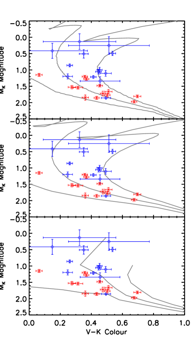
Figure 1: A colour-magnitude diagram of the 26 stars discussed within this work, plotted alongside three different sets of theoretical isochrones at 100, 500, and 800 Myrs. Those targets with new or refined orbits are plotted in blue with a diamond symbol (see Table 4), and those targets for which further measurements are required are plotted in red with a cross symbol (see Table 5 and §6.3). Three different sets of theoretical isochrones are plotted at ages of 100, 500, and 800 Myrs; (top) Lejeune & Schaerer (2001), (middle) Marigo et al. (2008), and (bottom) Siess et al. (2000).

Figure 2: The magnitude difference between primary and secondary for each binary system within this study as a function of angular separation. The targets are divided into two distinct subsamples, those with new or refined orbits estimated within this study (filled circles), and those for which further measurements are required before an orbital determination can be attempted (filled stars). The majority of the systems within the second subsample were newly resolved as a part of the VAST survey, demonstrating the higher dynamic range possible with AO imaging. The filled circles connected with a solid line represent companions within the same hierarchical triple (HIP 44127 and HIP 82321).

The sample of binaries is drawn from the ongoing VAST survey (De Rosa et al., 2011), an adaptive optics (AO) imaging survey of A-stars within 75 parsecs, and includes the 26 systems with projected separations less than 100 AU. The angular separations of the binaries range from 0$\aas@@fstack{\prime\prime}$094 to 4$\aas@@fstack{\prime\prime}$66, and 11 are newly resolved. Figure 2 plots the measured magnitude difference as a function of separation for the complete sample. Of the 26 systems, 13 have a substantial number of previous measurements, and these systems comprise the orbit subsample. For the remaining 13 systems, there is insufficient coverage to fit an orbit, and these binaries comprise the monitoring subsample. Table 1 lists each observed binary in the two subsamples, along with basic parameters for each such as distance (van Leeuwen, 2007), Tycho2 $V_{\rm T}$-band and 2MASS $K_{\rm s}$-band photometry (ESA, 1997; Skrutskie et al., 2006), and spectral type listed within the SIMBAD database.

For the brightest stars within the sample, the shortest 2MASS exposures saturate, requiring a different method for measuring the photometry, resulting in significantly larger uncertainties on the estimated magnitudes (Skrutskie et al., 2006). Therefore for three of these brighter targets, near-infrared photometry was obtained from alternative sources (Ducati, 2002; Morel & Magnenat, 1978), and converted into the 2MASS photometric bands using empirical colour transformations (Carpenter, 2001). The distribution of the sample on the color magnitude diagram (CMD) is plotted in Figure 1. Given the rapid evolution of massive stars off the Main Sequence, the position of an A-star on the CMD provides a method to estimate the age of the system based on a comparison with theoretical isochrones. The inferred age of the system from the CMD is combined with the dynamical system mass from the orbit and system photometry from the literature to test mass-magnitude relations at the corresponding age.

3 Observations

Table 2: Observing run details with calculated astrometric calibration values

Telescope	Date	Filter	Plate Scale		True North		Proposal ID
(Instrument)			(mas/px)		(∘)
CFHT	05/05/2001 – 07/05/2001	$H$ continuum	34.87$\pm$	0.14	1.47$\pm$	0.19	2001AF11
(KIR)	06/05/2001	$J$ continuum	34.82$\pm$	0.15	1.51$\pm$	0.17	2001AF11
	13/06/2008	H2 ($v=1-0$)	34.81$\pm$	0.10	-2.42$\pm$	0.13	2008AC22
	14/06/2008	FeII	34.76$\pm$	0.08	-2.40$\pm$	0.11	2008AC22
	30/08/2009 – 01/09/2009	H2 ($v=1-0$)	34.78$\pm$	0.10	-2.40$\pm$	0.20	2009BC06
	04/02/2010 – 05/02/2010	H2 ($v=1-0$)	34.75$\pm$	0.08	-2.37$\pm$	0.11	2010AC14
	2011	H2 ($v=1-0$)	34.77$\pm$	0.06	-2.35$\pm$	0.09	2011AC11
Gemini N	08/09/2008 – 14/11/2008	Br$\gamma$	21.28$\pm$	0.12	0.52$\pm$	0.29	GN-2008A-Q-74
(NIRI)	19/12/2009	Br$\gamma$	21.28$\pm$	0.12	0.52$\pm$	0.29	GN-2008B-Q-119
	25/06/2010 – 26/08/2010	Br$\gamma$	21.28$\pm$	0.12	0.52$\pm$	0.29	GN-2010A-Q-75
Lick	24/07/2008 – 25/07/2009	Br$\gamma$	74.55$\pm$	1.00	1.68$\pm$	0.50	–
(IRCAL)	16/10/2008 – 17/10/2008	Br$\gamma$	74.55$\pm$	1.00	1.68$\pm$	0.50	–
VLT-UT4	30/06/2004	IB218	27.02$\pm$	0.14	0.24$\pm$	0.30	272.D-5068(A)
(NACO)	10/01/2005	IB218	27.02$\pm$	0.15	0.26$\pm$	0.30	074.D-0180(A)
	08/02/2005	Ks	27.02$\pm$	0.15	0.26$\pm$	0.30	074.D-0180(A)
	08/11/2005	Ks	26.98$\pm$	0.08	0.21$\pm$	0.20	076.C-0270(A)
	10/11/2005	Ks	26.98$\pm$	0.08	0.21$\pm$	0.20	076.D-0108(A)
	06/12/2005	IB218	26.98$\pm$	0.08	0.21$\pm$	0.20	076.D-0108(A)
	04/01/2006	Ks	27.01$\pm$	0.13	0.31$\pm$	0.29	076.D-0108(A)
	07/01/2006	IB218	27.01$\pm$	0.13	0.31$\pm$	0.29	076.D-0108(A)
	27/04/2006	IB218	27.00$\pm$	0.12	0.09$\pm$	0.26	077.D-0147(A)
	20/09/2007	IB218	26.99$\pm$	0.12	-0.23$\pm$	0.21	080.D-0348(A)
	20/09/2007	Ks	26.99$\pm$	0.12	-0.23$\pm$	0.21	080.D-0348(A)
	26/09/2007	IB218	26.99$\pm$	0.12	-0.23$\pm$	0.21	080.D-0348(A)
	04/11/2007	Ks	27.00$\pm$	0.10	-0.18$\pm$	0.20	080.D-0348(A)
	15/02/2008	IB218	27.01$\pm$	0.14	-0.12$\pm$	0.29	080.D-0348(A)
	24/02/2008	Ks	27.01$\pm$	0.14	-0.12$\pm$	0.29	080.D-0348(A)
Palomar	11/04/2008	CH4	25.00$\pm$	1.00	0.70$\pm$	1.00	–
(PHARO)	12/04/2008	Br$\gamma$	25.00$\pm$	1.00	0.70$\pm$	1.00	–
	12/07/2008	CH4	25.00$\pm$	1.00	0.70$\pm$	1.00	–
	13/07/2008	Br$\gamma$	25.00$\pm$	1.00	0.70$\pm$	1.00	–
KIR – (Doyon et al., 1998)
NIRI (Near InfraRed Imager and Spectrometer) – (Hodapp et al., 2003)
IRCAL – (Lloyd et al., 2000)
NACO (Nasmyth Adaptive Optics System/ Near-Infrared Imager and Spectrograph) – (Lenzen et al., 2003; Rousset et al., 2003)
PHARO (Palomar High Angular Resolution Observer) – (Hayward et al., 2001)

With AO systems operating on telescopes ranging in diameter from the 3m Shane to the 8m Gemini and VLT, near-infrared images were obtained on all targets. In most cases, the filter used for the observations was a narrow or broadband filter within the $K$ bandpass, though some images were taken within the $J$ and $H$ bandpasses. Both the primary and secondary of the pairs were unsaturated in the AO images, simplifying the astrometry measurements. Table LABEL:tab:instruments details the key characteristics of the instruments used to acquire the new AO observations, with the measured pixel scale and orientation for each camera. A subset of the observations were obtained from the CFHT and ESO Science Archive Facilities. One measurement obtained at the Southern Observatory for Astrophysical Research (SOAR) as a part of the VAST survey, and used within this study, has been recently published in Hartkopf et al. (2012).

4 Data Analysis

4.1 AO image processing

The AO science images obtained were processed with standard image reduction steps including dark subtraction, flat fielding, interpolation over bad pixels and sky subtraction. To align all the images, the centroid of the bright primary was obtained in each exposure by fitting a Gaussian to the core of the central point spread function. For each system resolved within the observations, an empirical PSF was determined from the radial profile of the primary, after masking any close companion. The empirical PSF was then fit to the position and intensity of both components of the system, providing a measure of the separation, position angle, and magnitude difference. Uncertainties within the photometry and astrometry were estimated from the standard deviations of the photometric and astrometric measurements from each individual exposure before combination.

To ensure accurate determination of the separation and position angle, the pixel scale and orientation of the detectors were calibrated based on observations of the Trapezium cluster, with the exception of data obtained with IRCAL and PHARO. Depending on the total field-of-view of the detector, the positions of 20 to 40 Trapezium members were compared with the coordinates reported in McCaughrean & Stauffer (1994). The average derived pixel scale and orientation were computed, and the standard deviation of these values were used as the associated errors; the results are given in Table LABEL:tab:instruments. For the data obtained with IRCAL and PHARO, the pixel scale and orientation were calibrated from binary systems also observed with instruments calibrated with Trapezium measurements.

4.2 Orbital determination

For the 13 binaries with sufficient coverage of the orbit, a fit was performed for the orbital elements and an estimate of the dynamical mass was determined. The measurements presented within this study were combined with previous measurements contained within the Washington Double Star (WDS; Mason et al., 2001) Catalog. These archive measurements were obtained using a variety of observational techniques, and date back to the 18^th Century. As in some cases the statistical uncertainties were not provided in the WDS Catalog, we searched the literature for the formal errors for each individual measurement, and only separation and position angle values for which uncertainties could be assigned were included within the fitting procedure. A detailed listing of the individual measurements used for the orbital determination will be made available at the Strasbourg astronomical Data Center (CDS - http://cds.u-strasbg.fr).

Our orbit fitting approach utilises the method presented by Hilditch (2001), and demonstrated by an application to measurements of the T Tau S system (Köhler et al., 2008). This method is similar to the grid-based search technique developed by Hartkopf et al. (1989). At each epoch of observation $t_{i}$, the $x_{i}$,$y_{i}$ position of the companion with respect to the primary is measured in the observed tangent plane. These values are related to the true position of the secondary in the orbital plane ($x_{i}^{\prime}$,$y_{i}^{\prime}$) through the following equations

$$\begin{split}x_{i}&=Ax_{i}^{\prime}+Fy_{i}^{\prime}\\ y_{i}&=Bx_{i}^{\prime}+Gy_{i}^{\prime}\end{split}$$ (1)

where $A$, $B$, $F$ and $G$ are the orbital Thiele-Innes elements, with

$$\begin{split}A&=a(\cos\omega\cos\Omega-\sin\omega\sin\Omega\cos i)\\ B&=a(\cos\omega\sin\Omega+\sin\omega\cos\Omega\cos i)\\ F&=a(-\sin\omega\cos\Omega-\cos\omega\sin\Omega\cos i)\\ G&=a(-\sin\omega\sin\Omega+\cos\omega\cos\Omega\cos i)\end{split}$$ (2)

where $a$ is the semi-major axis of the orbit, $\omega$ the longitude of periastron, $\Omega$ the longitude of the ascending node, and $i$ the inclination – four of the seven orbital elements. The position of the companion in the orbital plane ($x_{i}^{\prime}$,$y_{i}^{\prime}$) can also be expressed through the remaining orbital elements ($e$, $P$, $T_{0}$) as

$$\begin{split}x_{i}^{\prime}&=\cos E-e\\ y_{i}^{\prime}&=\sqrt{1-e^{2}}\sin E\end{split}$$ (3)

where $e$ is the eccentricity of the system. The eccentric anomaly ($E$) can be determined from a numerical solution to Kepler’s equation

$$\begin{split}M&=E-e\sin E\\ &=(2\pi/P)(t_{i}-T_{0})\end{split}$$ (4)

where $M$ is the mean anomaly, $P$ the period of the system, and $T_{0}$ the epoch of periastron passage. At each epoch of observation, the position of the component in the orbital plane can be defined using just three of the orbital elements ($e$, $P$, and $T_{0}$). The orbital position at each epoch can then be converted into the observed position using the equations in Equation 1 through a least-squares determination of the four Thiele-Innes elements.

An initial estimation of the orbital parameters of each system can be determined through an iterative three-dimensional grid search of $e$, $P$, and $T_{0}$. A wider range of parameter values were searched, with 100 linear steps searched over a range of $0\leq e<1$, 500 linear steps between $1\leq\log(P[yrs])\leq 3$, and $T_{0}$ initially distributed between the years $2000.0-(P/2)$ and $2000.0+(P/2)$. At each position within this three-dimensional grid, the fit orbital positions ($x_{i}^{\prime}$,$y_{i}^{\prime}$) were directly calculated (Eqn. 3), with the four remaining orbital parameters ($a$, $i$, $\omega$, $\Omega$) estimated from a least-squares fit to the observed positions using Equations 1 and 2. After the $\chi^{2}$ statistic was calculated at each position within the grid, the range of $T_{0}$ values searched was reduced by a factor of 10 centred on the optimum value of $T_{0}$ found within the previous iteration. This process was repeated until the step size in $T_{0}$ was reduced to less than one day. The values for $a$, $i$, $\omega$ and $\Omega$ can be determined from an inversion of Equation 2 (Green, 1985),

$$\begin{split}\Omega&=\frac{1}{2}\left(\arctan\left(\frac{B-F}{G+A}\right)-\arctan\left(\frac{B+F}{G-A}\right)\right)\\ \omega&=\left(\arctan\left(\frac{B-F}{G+A}\right)-\Omega\right)\\ i&=2\arctan\left[\sqrt{\frac{-\left(B+F\right)\sin\left(\omega+\Omega\right)}{\left(B-F\right)\sin\left(\omega-\Omega\right)}}\right]\\ a&=\frac{B-F}{\sin\left(\omega+\Omega\right)\left(1+\cos\left(i\right)\right)}\end{split}$$ (5)

The orbital parameters calculated at each position within the ($P$, $e$) grid are then used as a starting point for a Levenberg-Marquardt minimisation to ensure the minimum of the $\chi^{2}$ distribution is found. The set of orbital parameters with the minimum $\chi^{2}$ statistic was then used as the orbit solution for the system.

The shape of the $\chi^{2}$ distribution in the vicinity of the global minimum can be used to determine the 1$\sigma$ uncertainties of each parameter (Press et al., 1992). By perturbing an individual parameter away from the global minimum, and optimising the remaining parameters, a region of the $\chi^{2}$ distribution can be calculated where the $\chi^{2}$ statistic is less than $\chi^{2}_{\rm min}+1$. This region encloses 68% of the probability distribution, and is not necessarily symmetric about the minimum $\chi^{2}$ value. Our implementation of the orbit fitting method was tested against four well studied systems (Bonnefoy et al., 2009; Dupuy et al., 2009; Liu et al., 2008), with the resulting parameters being within the published 1$\sigma$ uncertainties.

4.3 Theoretical mass-magnitude relations

Table 3: Summary of theoretical model grids

Grid	Mass Range		Metallicity
reference	(M⊙)		($Z$)
Lejeune & Schaerer (2001)	$0.80$ $<M<$	$5.0$	0.02
Marigo et al. (2008)	$0.15$ $<M<$	$5.0$	0.02
Siess et al. (2000)	$0.10$ $<M<$	$5.0$	0.02
Baraffe et al. (1998)	$0.08$ $<M<$	$1.5$	0.02

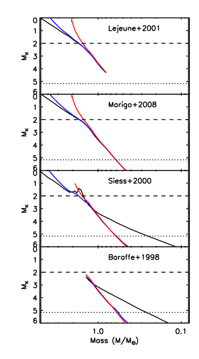
Figure 3: Mass-magnitude relations were constructed from each of the four model grids. The evolution of the mass-magnitude relation is shown for each grid, with the 10 Myr (black line), 100 Myr (blue line) and 1 Gyr (red line) relations plotted. For reference the dashed line indicates the faintest A-type star within the sample, and the dotted line indicates the Zero-Age Main Sequence magnitude of an M0 star. A-type stars typically have an absolute $K$-band magnitude ranging between $M_{K}=0$ and $M_{K}=2$, where the mass is significantly dependent on the age of the star. Within the Lejeune & Schaerer (2001) and Marigo et al. (2008) models, the mass-magnitude relation of stars fainter than $M_{K}\sim 2$ is not dependent on the age of the star. The Siess et al. (2000) and Baraffe et al. (1998) models include a description of the contraction phase of lower-mass stars onto the Main Sequence during the early portion of its life.

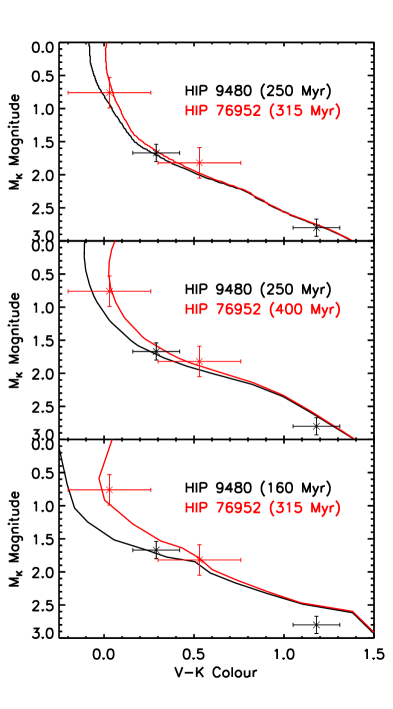
Figure 4: The age of each system can be estimated based on the position of each component on the colour-magnitude diagram (top - Lejeune & Schaerer (2001), middle - Marigo et al. (2008), bottom - Siess et al. (2000)). This procedure, while demonstrated for only two systems in this figure, was repeated for all the remaining members of the orbit subsample. For each system, the age estimated from each of the three model grids is reported in Table 10.

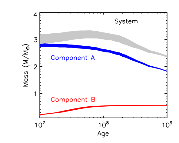
Figure 5: The mass-magnitude relation for a hypothetical binary system with $M_{K}({\rm A})=1.25\pm 0.05$ and $M_{K}({\rm B})=5.50\pm 0.10$, as a function of system age. The evolution of the mass-magnitude relation is shown for both components (A - blue region, B - red region), and the system as a whole (grey region). The extent of the region in each case represents the uncertainty in the mass estimate due to the uncertainties of the magnitudes of each component.

We obtained four different grids of evolutionary models with which the dynamical system masses estimated from the fitted orbital parameters were compared. Table LABEL:tab:models lists the mass range, metallicity, and literature reference for each of the four grids. The Lejeune & Schaerer (2001), Marigo et al. (2008), and Siess et al. (2000) grids covers a significant portion of the lifespan of a typical A-type star, and as such we applied a maximum age cut-off at 1 Gyr. In addition to these grids, models from Baraffe et al. (1998) were obtained in order to study a pair of lower-mass companions presented in §6.1.2. Each grid was converted into the photometric systems used within this study - Tycho $V$ and 2MASS $K_{S}$ (Carpenter, 2001), before producing a high resolution ($dM/M_{\odot}=0.001$) mass-magnitude relation, created through cubic interpolation of the grid data, as shown in Figure 3.

The absolute $V$- and $K$-band magnitudes were calculated from the $V$-band magnitude differences obtained from the literature, and the $K$-band magnitude differences presented within this study (Tables 4 and 5). The individual component magnitudes and $V-K$ colour for each system are presented in Table 6. Within the A-type star mass range, the mass-magnitude relations significantly change as a function of the age of the system due to the rapid evolution of A-type stars across the CMD. The age of each system is therefore estimated, based on the position of the primary on the CMD (Figure 4), before a mass for each component is estimated from the mass-magnitude relations. The estimated masses of each component are summed to produce an estimation of the system mass, hereafter called the theoretical system mass.

To demonstrate the analysis procedure, a hypothetical binary system of magnitudes $M_{K}({\rm A})=1.25$, $M_{K}({\rm B})=5.50$ was used to construct the mass-age relation for each component, and their corresponding sum (Figure 5). The evolution of the mass-magnitude relation as a function of age can be then visualised as a continuous function for both components within the system. For this example a set of models were used which includes the pre-Main Sequence (PMS) contraction phase of lower-mass stars, as demonstrated by the increase in the derived mass as a function of age for the companion. The two mass-age curves can then be summed to produce a mass-age relation for the system in question. Using the age estimated for the system based upon its position on the CMD, a theoretical system mass can be estimated and compared with the dynamical system mass determined from the orbital elements.

5 Results

5.1 Astrometric results

Table 4: Measured binary position angle and separation for previously resolved systems

HIP	Comp.	WDS	Discoverer	Previous	Instrument	Epoch	$\theta$		$\rho$		$\Delta K$
		Designation	Designation	Orbit			(deg)		(arcsec)		(mag)
5300	AB	01078-4129	RST3352	Söderhjelm (1999)	NACO	2005.02	15.73$\pm$	0.76	0.089$\pm$	0.001	0.507$\pm$	0.020
					NACO	2007.72	126.69$\pm$	0.38	0.114$\pm$	0.001	*0.573$\pm$	0.018
9480	A-B	02020+7054	BU 513	Mason et al. (1999)	IRCAL	2008.79	293.97$\pm$	0.75	0.679$\pm$	0.011	1.110$\pm$	0.056
					KIR	2009.67	297.36$\pm$	0.22	0.666$\pm$	0.002	1.172$\pm$	0.013
					NIRI	2010.65	302.11$\pm$	0.29	0.644$\pm$	0.004	*1.137$\pm$	0.007
11569	Aa,Ab	02291+6724	CHR 6	Drummond et al. (2003)	IRCAL	2008.79	43.50$\pm$	0.80	0.575$\pm$	0.006	*1.906$\pm$	0.026
					KIR	2010.10	41.52$\pm$	2.61	0.602$\pm$	0.023	1.771$\pm$	0.301
17954	AB	03503+2535	STT 65	Docobo & Ling (2007)	NIRI	2008.87	194.76$\pm$	0.31	0.200$\pm$	0.001	*0.232$\pm$	0.005
28614	AB	06024+0939	A 2715	Muterspaugh et al. (2008)	NIRI	2009.96	21.95$\pm$	0.29	0.403$\pm$	0.002	*1.008$\pm$	0.006
					KIR	2011.31	21.31$\pm$	1.06	0.397$\pm$	0.006	0.896$\pm$	0.120
36850	AB	07346+3153	STF1110	Docobo & Costa (1985)	KIR	2010.09	57.46$\pm$	0.14	4.663$\pm$	0.013	*0.698$\pm$	0.050
44127	BC	08592+4803	HU 628	Eggen (1967)	PHARO	2008.28	242.01$\pm$	1.04	0.433$\pm$	0.017	*0.005$\pm$	0.031
					KIR	2010.10	228.98$\pm$	0.27	0.568$\pm$	0.003	0.027$\pm$	0.023
					KIR	2011.30	223.37$\pm$	0.31	0.656$\pm$	0.003	-0.011$\pm$	0.039
47479	AB	09407-5759	B 780	Söderhjelm (1999)	NACO	2008.12	300.22$\pm$	0.58	0.099$\pm$	0.001	*0.082$\pm$	0.017
76952	AB	15427+2618	STF1967	Muterspaugh et al. (2010)	PHARO	2008.28	112.65$\pm$	1.07	0.683$\pm$	0.028	-
					KIR	2011.31	111.37$\pm$	0.33	0.620$\pm$	0.005	*1.056$\pm$	0.030
77660	AB	15513-0305	CHR 51	Docobo et al. (2010)	KIR	2001.34	82.72$\pm$	2.42	0.188$\pm$	0.018	-
					KIR	2001.34	81.97$\pm$	1.59	0.197$\pm$	0.008	-
					KIR	2001.35	83.38$\pm$	3.67	0.185$\pm$	0.016	-
					NACO	2004.50	71.87$\pm$	0.31	0.247$\pm$	0.001	*1.487$\pm$	0.006
					NACO	2006.32	69.74$\pm$	0.42	0.274$\pm$	0.003	1.472$\pm$	0.097
					KIR	2010.10	66.69$\pm$	0.47	0.330$\pm$	0.004	1.483$\pm$	0.058
					KIR	2011.30	64.21$\pm$	2.57	0.340$\pm$	0.014	1.455$\pm$	0.194
80628	Ab,Ab	16278-0822	RST3949	-	PHARO	2008.28	22.56$\pm$	1.05	0.674$\pm$	0.027	*2.072$\pm$	0.066
					IRCAL	2008.56	23.53$\pm$	0.71	0.685$\pm$	0.009	1.978$\pm$	0.057
					KIR	2011.31	34.37$\pm$	0.29	0.771$\pm$	0.003	2.237$\pm$	0.038
82321	BC	16492+4559	A 1866	Popovic (1969)	PHARO	2008.53	247.33$\pm$	1.03	0.286$\pm$	0.012	-
					KIR	2011.30	260.51$\pm$	0.53	0.301$\pm$	0.005	*0.299$\pm$	0.044
93506	AB	19026-2953	HDO 150	Mason et al. (1999)	KIR	2008.45	31.05$\pm$	2.31	0.194$\pm$	0.010	-
					KIR	2011.31	285.59$\pm$	0.71	0.304$\pm$	0.004	*0.320$\pm$	0.043
* - Photometry measurement used to determine the magnitude of each component in Table 6.

Table 5: Measured binary position angle and separation for potential orbital monitoring targets

HIP	Instrument	Epoch	$\theta$		$\rho$		$\Delta K$		Projected
			(deg)		(arcsec)		(mag)		Separation (AU)
128	NIRI	2008.72	80.64$\pm$	0.29	0.983$\pm$	0.006	*3.521$\pm$	0.021	69.59$\pm$	1.72
	IRCAL	2008.79	80.73$\pm$	0.52	0.975$\pm$	0.013	3.355$\pm$	0.037	68.98$\pm$	1.90
2381	NACO	2005.93	279.51$\pm$	0.26	1.765$\pm$	0.006	*6.206$\pm$	0.088	93.75$\pm$	1.48
	NACO	2007.73	279.13$\pm$	0.22	1.767$\pm$	0.008	6.229$\pm$	0.055	93.86$\pm$	1.51
	NIRI	2008.79	278.54$\pm$	0.29	1.759$\pm$	0.013	7.401$\pm$	0.711	93.39$\pm$	1.59
2852	NIRI	2008.79	260.55$\pm$	0.30	0.931$\pm$	0.006	*5.001$\pm$	0.056	45.51$\pm$	0.82
5310	NIRI	2008.79	174.99$\pm$	0.30	0.357$\pm$	0.002	*3.719$\pm$	0.023	16.88$\pm$	0.62
18217	IRCAL	2008.79	64.78$\pm$	0.65	1.037$\pm$	0.012	2.301$\pm$	0.029	52.37$\pm$	1.24
	NIRI	2008.87	64.96$\pm$	0.29	1.033$\pm$	0.006	*2.41$\pm$	0.010	52.13$\pm$	1.12
29852	NACO	2005.85	210.76$\pm$	0.22	0.218$\pm$	0.001	*2.003$\pm$	0.013	13.49$\pm$	0.21
	NACO	2005.86	210.80$\pm$	0.21	0.217$\pm$	0.001	1.983$\pm$	0.012	13.44$\pm$	0.21
51384	PHARO	2008.18	212.43$\pm$	1.05	2.078$\pm$	0.084	*4.543$\pm$	0.169	84.44$\pm$	3.66
65241	NACO	2005.10	196.95$\pm$	0.62	0.328$\pm$	0.003	3.061$\pm$	0.231	21.65$\pm$	0.50
	NACO	2008.15	212.75$\pm$	0.57	0.258$\pm$	0.003	*3.025$\pm$	0.097	17.01$\pm$	0.42
66223	PHARO	2008.53	187.71$\pm$	1.02	1.381$\pm$	0.056	*5.660$\pm$	0.105	96.42$\pm$	4.73
103298	NIRI	2008.69	115.72$\pm$	0.30	0.220$\pm$	0.001	*2.962$\pm$	0.007	13.29$\pm$	0.25
109667	NIRI	2008.69	285.17$\pm$	0.30	1.117$\pm$	0.007	*3.997$\pm$	0.011	70.88$\pm$	2.38
	KIR	2009.66	284.66$\pm$	0.25	1.108$\pm$	0.006	4.051$\pm$	0.073	70.28$\pm$	2.35
	NIRI	2010.48	284.38$\pm$	0.29	1.101$\pm$	0.007	4.044$\pm$	0.103	69.84$\pm$	2.34
110787	NIRI	2008.71	211.11$\pm$	0.35	0.291$\pm$	0.002	*3.891$\pm$	0.043	18.38$\pm$	0.29
116611	NIRI	2008.75	173.11$\pm$	0.32	0.950$\pm$	0.006	*5.930$\pm$	0.089	67.78$\pm$	1.38
	NIRI	2010.48	172.11$\pm$	0.34	0.943$\pm$	0.006	5.794$\pm$	0.076	67.31$\pm$	1.34
* - Photometry measurement used to determine the magnitude of each component in Table 6.

Table 6: Derived parameters of individual components

HIP

Comp.

$V_{\rm T}$

$K_{\rm S}$

$V-K$

${\rm M}_{V}$

${\rm M}_{K}$

Additional

SB

Reference

(mag)

(mag)

(mag)

(mag)

Components

Type

Orbit Subsample

5300

A

5.51$\pm$

0.02

5.28$\pm$

0.02

0.23$\pm$

0.03

1.73$\pm$

0.08

1.50$\pm$

0.08

B

6.85$\pm$

0.08

5.85$\pm$

0.02

0.99$\pm$

0.08

3.07$\pm$

0.11

2.08$\pm$

0.08

9480†

A

4.69$\pm$

0.01

4.40$\pm$

0.13

0.29$\pm$

0.13

1.95$\pm$

0.03

1.67$\pm$

0.13

B

6.72$\pm$

0.01

5.54$\pm$

0.13

1.18$\pm$

0.13

3.98$\pm$

0.04

2.80$\pm$

0.13

11569 ‡

Aa

4.67$\pm$

0.01

4.79$\pm$

0.03

-0.12$\pm$

0.03

1.62$\pm$

0.07

1.74$\pm$

0.08

Ab

8.65$\pm$

0.16

6.71$\pm$

0.03

1.94$\pm$

0.16

5.60$\pm$

0.17

3.66$\pm$

0.08

17954

A

5.81$\pm$

0.04

5.46$\pm$

0.02

0.35$\pm$

0.04

2.05$\pm$

0.08

1.70$\pm$

0.07

B

6.26$\pm$

0.06

5.69$\pm$

0.02

0.57$\pm$

0.06

2.50$\pm$

0.09

1.93$\pm$

0.07

28614

A

4.32$\pm$

0.01

4.00$\pm$

0.26

0.33$\pm$

0.26

0.94$\pm$

0.07

0.61$\pm$

0.27

Aa, Ab

SB1

Fekel et al. (2002)

B

6.22$\pm$

0.02

5.01$\pm$

0.26

1.22$\pm$

0.26

2.84$\pm$

0.07

1.62$\pm$

0.27

Ba, Bb

SB2

Fekel et al. (2002)

36850

A

1.98$\pm$

0.02

1.93$\pm$

0.03

0.05$\pm$

0.04

1.02$\pm$

0.13

0.97$\pm$

0.13

Aa, Ab

SB1

Vinter Hansen et al. (1940)

B

2.88$\pm$

0.03

2.63$\pm$

0.04

0.25$\pm$

0.05

1.92$\pm$

0.13

1.66$\pm$

0.13

Ba, Bb

SB1

Vinter Hansen et al. (1940)

44127

A

3.16$\pm$

0.02

2.71$\pm$

0.03

0.45$\pm$

0.04

2.35$\pm$

0.02

1.90$\pm$

0.03

B

10.88$\pm$

0.11

6.90$\pm$

0.04

3.98$\pm$

0.12

10.07$\pm$

0.11

6.09$\pm$

0.04

C

11.08$\pm$

0.12

6.90$\pm$

0.04

4.18$\pm$

0.12

10.27$\pm$

0.12

6.09$\pm$

0.04

47479

A

5.82$\pm$

0.01

5.51$\pm$

0.02

0.31$\pm$

0.02

1.51$\pm$

0.07

1.21$\pm$

0.07

B

6.45$\pm$

0.01

5.59$\pm$

0.02

0.85$\pm$

0.03

2.14$\pm$

0.07

1.29$\pm$

0.07

76952

A

4.05$\pm$

0.01

4.02$\pm$

0.23

0.03$\pm$

0.23

0.80$\pm$

0.05

0.76$\pm$

0.23

B

5.60$\pm$

0.02

5.07$\pm$

0.23

0.53$\pm$

0.23

2.35$\pm$

0.05

1.82$\pm$

0.23

77660

A

5.21$\pm$

0.01

4.94$\pm$

0.02

0.26$\pm$

0.02

1.72$\pm$

0.04

1.46$\pm$

0.04

B

7.82$\pm$

0.04

6.43$\pm$

0.02

1.38$\pm$

0.04

4.33$\pm$

0.05

2.95$\pm$

0.04

80628

Aa

4.68$\pm$

0.01

4.32$\pm$

0.04

0.37$\pm$

0.04

1.62$\pm$

0.08

1.25$\pm$

0.09

Aa1, Aa2

SB2

Gutmann (1965)

Ab

8.80$\pm$

0.10

6.39$\pm$

0.07

2.41$\pm$

0.12

5.74$\pm$

0.13

3.33$\pm$

0.11

82321

A

4.87$\pm$

0.01

4.73$\pm$

0.02

0.14$\pm$

0.02

1.16$\pm$

0.04

1.02$\pm$

0.04

B

9.19$\pm$

0.11

7.33$\pm$

0.03

1.86$\pm$

0.11

5.47$\pm$

0.12

3.62$\pm$

0.05

C

9.29$\pm$

0.11

7.63$\pm$

0.04

1.66$\pm$

0.12

5.57$\pm$

0.12

3.92$\pm$

0.05

93506

A

3.27$\pm$

0.01

2.90$\pm$

0.23

0.37$\pm$

0.23

1.11$\pm$

0.05

0.74$\pm$

0.24

B

3.48$\pm$

0.01

3.22$\pm$

0.24

0.26$\pm$

0.24

1.32$\pm$

0.05

1.06$\pm$

0.24

Monitoring Subsample

128

AB

–

6.06$\pm$

0.02

–

–

1.81$\pm$

0.06

A, B

SB1

Carquillat et al. (2003)

C

–

9.58$\pm$

0.03

–

–

5.33$\pm$

0.06

2381

A

–

4.83$\pm$

0.02

–

–

1.21$\pm$

0.04

B

–

11.04$\pm$

0.09

–

–

7.41$\pm$

0.10

2852

A

–

5.43$\pm$

0.02

–

–

1.98$\pm$

0.04

B

–

10.43$\pm$

0.06

–

–

6.98$\pm$

0.07

5310

A

–

5.25$\pm$

0.02

–

–

1.88$\pm$

0.08

B

–

8.97$\pm$

0.03

–

–

5.60$\pm$

0.08

18217

A

–

5.48$\pm$

0.02

–

–

1.97$\pm$

0.05

B

–

7.90$\pm$

0.02

–

–

4.38$\pm$

0.05

29852

A

–

5.60$\pm$

0.02

–

–

1.64$\pm$

0.04

B

–

7.60$\pm$

0.02

–

–

3.64$\pm$

0.04

51384

A

–

4.87$\pm$

0.02

–

–

1.82$\pm$

0.04

B

–

9.41$\pm$

0.17

–

–

6.37$\pm$

0.17

65241

A

–

5.69$\pm$

0.02

–

–

1.59$\pm$

0.05

B

–

8.71$\pm$

0.09

–

–

4.62$\pm$

0.11

66223

Aa

–

5.89$\pm$

0.02

–

–

1.67$\pm$

0.06

Ab

–

11.55$\pm$

0.11

–

–

7.33$\pm$

0.12

103298

Aa

–

5.26$\pm$

0.02

–

–

1.35$\pm$

0.04

Ab

–

8.22$\pm$

0.02

–

–

4.31$\pm$

0.04

109667

A

–

5.76$\pm$

0.02

–

–

1.75$\pm$

0.07

B

–

9.76$\pm$

0.02

–

–

5.75$\pm$

0.07

110787

A

–

5.57$\pm$

0.03

–

–

1.57$\pm$

0.04

B

–

9.46$\pm$

0.05

–

–

5.46$\pm$

0.06

116611

Aa

–

5.42$\pm$

0.02

–

–

1.16$\pm$

0.05

Aa1, Aa2

SB1

Rucinski et al. (2005)

Ab

–

11.35$\pm$

0.09

–

–

7.09$\pm$

0.10

† - The spectroscopic binary reported by Abt (1965) is the system resolved within the AO data.

‡ - The individual component magnitudes may be significantly biased due to the presence of additional companions within the resolution limit of the

Tycho2 and 2MASS observations.

Table 7: Visual magnitude differences for a subset of the sample

HIP	$\Delta V$		Reference
5300	1.34$\pm$	0.10*	Horch et al. (2001)
9480	2.03$\pm$	0.01	Fabricius & Makarov (2000)
11569	3.98$\pm$	0.16	Christou & Drummond (2006)
17954	0.45$\pm$	0.10*	Horch et al. (2004)
28614	1.90$\pm$	0.02	Fabricius & Makarov (2000)
36850	0.90$\pm$	0.03	Worley (1969)
44127 A,BC	7.06$\pm$	0.10*	Baize & Petit (1989)
44127 BC	0.20$\pm$	0.10*	Mason et al. (2001)
47479	0.63$\pm$	0.02	Mason et al. (2001)
76952	1.55$\pm$	0.02	Fabricius & Makarov (2000)
77660	2.61$\pm$	0.04	Docobo et al. (2010)
80628	4.12$\pm$	0.10*	Mason et al. (2001)
82321 A,BC	3.61$\pm$	0.10*	Mason et al. (2001)
83231 BC	0.10$\pm$	0.10*	Mason et al. (2001)
93506	0.21$\pm$	0.02	Fabricius & Makarov (2000)
* - For $\Delta$V measurements without uncertainties, 0.10 is used

The astrometry and photometry measurements of the two subsamples are given in Tables 4 and 5. Both tables contain the Hipparcos designation of the primary, the components of the system under investigation, the instrument and epoch of observation, and the measured astrometric values with corresponding uncertainties. For the orbit subsample, the WDS designation and discoverer code are also listed for reference.

Combining the $K$-band magnitudes of the sample with the $\Delta K$ values reported in Tables 4 and 5, and the Hipparcos parallax, allowed for an estimation of the $K$-band apparent and absolute magnitudes of the resolved components (Table 6). For systems with $\Delta V$ measurements reported within the literature (Table 7), the corresponding estimated $V$-band apparent and absolute magnitudes, and $V-K$ colours for each resolved component are reported. Seven members of the overall sample are hierarchical systems with at least one of the components resolved within our dataset consisting of multiple sub-components, indicated in Table 6. An example of this is HIP 128; our AO data are able to resolve a previously-unknown binary companion within this system (HIP 128 C at $\sim 1\aas@@fstack{\prime\prime}0$), but are of insufficient angular resolution to resolve the previously-known spectroscopic component HIP 128 B. Without an estimate of the $\Delta V$ or $\Delta K$ between HIP 128 A and HIP 128 B, the individual magnitudes cannot be estimated and therefore only the blended magnitudes of the two components are listed.

5.2 Orbital elements and dynamical masses

Table 8: Estimated orbital parameters and corresponding 1$\sigma$ uncertainties

HIP	N.	Period		Semi-major		Inclination		Longitude		Epoch of		Eccentricity		Longitude		System
	Meas.			axis				of Node		Periastron				of Periastron		Mass
		$P$ (yrs)		$a$ ($\arcsec$)		$i$ (∘)		$\Omega$ (∘)		$T_{0}$ (yrs)		$e$		$\omega$ (∘)		(M⊙)
5300	19	28.36${}^{+}_{-}$	${}^{0.04}_{0.04}$	0.2396${}^{+}_{-}$	${}^{0.0005}_{0.0005}$	65.3${}^{+}_{-}$	${}^{0.3}_{0.3}$	142.7${}^{+}_{-}$	${}^{0.3}_{0.3}$	2007.94${}^{+}_{-}$	${}^{0.02}_{0.02}$	0.424${}^{+}_{-}$	${}^{0.002}_{0.002}$	333.9${}^{+}_{-}$	${}^{0.4}_{0.3}$	3.16$\pm$	0.34
9480	66	61.14${}^{+}_{-}$	${}^{0.05}_{0.05}$	0.614${}^{+}_{-}$	${}^{0.002}_{0.002}$	16.7${}^{+}_{-}$	${}^{0.9}_{0.9}$	48.2${}^{+}_{-}$	${}^{3.3}_{3.1}$	1964.35${}^{+}_{-}$	${}^{0.09}_{0.09}$	0.355${}^{+}_{-}$	${}^{0.001}_{0.001}$	19.5${}^{+}_{-}$	${}^{3.5}_{3.7}$	2.72$\pm$	0.13
11569	11	50.2${}^{+}_{-}$	${}^{1.0}_{1.0}$	0.429${}^{+}_{-}$	${}^{0.007}_{0.007}$	149.0${}^{+}_{-}$	${}^{1.7}_{1.6}$	180.0${}^{+}_{-}$	${}^{2.7}_{2.8}$	1993.24${}^{+}_{-}$	${}^{0.08}_{0.08}$	0.642${}^{+}_{-}$	${}^{0.009}_{0.009}$	331.3${}^{+}_{-}$	${}^{2.6}_{2.7}$	2.12$\pm$	0.25
17954	44	61.2${}^{+}_{-}$	${}^{0.1}_{0.1}$	0.442${}^{+}_{-}$	${}^{0.002}_{0.002}$	84.7${}^{+}_{-}$	${}^{0.1}_{0.1}$	26.4${}^{+}_{-}$	${}^{0.2}_{0.2}$	1998.30${}^{+}_{-}$	${}^{0.08}_{0.08}$	0.628${}^{+}_{-}$	${}^{0.002}_{0.002}$	340.3${}^{+}_{-}$	${}^{0.7}_{0.7}$	4.15$\pm$	0.39
28614	69	18.641${}^{+}_{-}$	${}^{0.008}_{0.008}$	0.2741${}^{+}_{-}$	${}^{0.0001}_{0.0001}$	96.59${}^{+}_{-}$	${}^{0.02}_{0.02}$	24.76${}^{+}_{-}$	${}^{0.02}_{0.02}$	2003.742${}^{+}_{-}$	${}^{0.004}_{0.004}$	0.744${}^{+}_{-}$	${}^{0.001}_{0.001}$	217.08${}^{+}_{-}$	${}^{0.08}_{0.08}$	6.36$\pm$	0.62
36850	207	466.8${}^{+}_{-}$	${}^{6.3}_{6.1}$	6.78${}^{+}_{-}$	${}^{0.05}_{0.05}$	113.56${}^{+}_{-}$	${}^{0.09}_{0.09}$	41.2${}^{+}_{-}$	${}^{0.1}_{0.1}$	1957.3${}^{+}_{-}$	${}^{0.3}_{0.3}$	0.333${}^{+}_{-}$	${}^{0.007}_{0.006}$	249.3${}^{+}_{-}$	${}^{0.6}_{0.5}$	5.42$\pm$	0.97
44127	9	39.4${}^{+}_{-}$	${}^{0.1}_{0.1}$	0.70${}^{+}_{-}$	${}^{0.01}_{0.01}$	111.6${}^{+}_{-}$	${}^{1.1}_{1.1}$	24.5${}^{+}_{-}$	${}^{1.2}_{1.3}$	1999.1${}^{+}_{-}$	${}^{0.6}_{0.7}$	0.35${}^{+}_{-}$	${}^{0.02}_{0.02}$	354.2${}^{+}_{-}$	${}^{4.4}_{4.7}$	0.68$\pm$	0.04
47479	5	10.74${}^{+}_{-}$	${}^{0.04}_{0.04}$	0.1207${}^{+}_{-}$	${}^{0.0006}_{0.0006}$	128.4${}^{+}_{-}$	${}^{1.5}_{1.4}$	87.4${}^{+}_{-}$	${}^{0.5}_{0.5}$	2005.89${}^{+}_{-}$	${}^{0.03}_{0.04}$	0.365${}^{+}_{-}$	${}^{0.009}_{0.009}$	18.6${}^{+}_{-}$	${}^{1.1}_{1.2}$	5.83$\pm$	0.53
76952	104	91.2${}^{+}_{-}$	${}^{0.4}_{0.4}$	0.729${}^{+}_{-}$	${}^{0.006}_{0.006}$	94.45${}^{+}_{-}$	${}^{0.07}_{0.07}$	111.75${}^{+}_{-}$	${}^{0.09}_{0.09}$	1931.6${}^{+}_{-}$	${}^{0.3}_{0.3}$	0.48${}^{+}_{-}$	${}^{0.01}_{0.01}$	103.8${}^{+}_{-}$	${}^{0.6}_{0.5}$	4.19$\pm$	0.30
80628	8	82.8${}^{+}_{-}$	${}^{1.5}_{1.3}$	0.79${}^{+}_{-}$	${}^{0.03}_{0.02}$	31.2${}^{+}_{-}$	${}^{5.4}_{6.0}$	86.8${}^{+}_{-}$	${}^{8.1}_{5.6}$	1994.1${}^{+}_{-}$	${}^{0.9}_{1.1}$	0.45${}^{+}_{-}$	${}^{0.03}_{0.03}$	177.9${}^{+}_{-}$	${}^{6.8}_{7.9}$	4.99$\pm$	0.75
82321	12	56.4${}^{+}_{-}$	${}^{0.3}_{0.3}$	0.279${}^{+}_{-}$	${}^{0.005}_{0.005}$	37.4${}^{+}_{-}$	${}^{2.6}_{2.8}$	57.5${}^{+}_{-}$	${}^{5.9}_{6.1}$	1991.2${}^{+}_{-}$	${}^{2.3}_{2.1}$	0.13${}^{+}_{-}$	${}^{0.02}_{0.02}$	69.4${}^{+}_{-}$	${}^{8.0}_{7.5}$	1.16$\pm$	0.09
93506	42	21.00${}^{+}_{-}$	${}^{0.01}_{0.01}$	0.489${}^{+}_{-}$	${}^{0.001}_{0.001}$	111.1${}^{+}_{-}$	${}^{0.1}_{0.1}$	74.0${}^{+}_{-}$	${}^{0.1}_{0.1}$	2005.99${}^{+}_{-}$	${}^{0.03}_{0.03}$	0.211${}^{+}_{-}$	${}^{0.001}_{0.001}$	7.2${}^{+}_{-}$	${}^{0.6}_{0.6}$	5.26$\pm$	0.37

Table 9: Previous and revised dynamical system masses

HIP	Old Estimate		New Estimate
	(M⊙)		(M⊙)
5300	3.45		3.16$\pm$	0.34
9480	2.98$\pm$	0.39	2.72$\pm$	0.13
11569	2.12$\pm$	0.33	2.12$\pm$	0.25
17954	3.37$\pm$	0.35	4.15$\pm$	0.39
28614	6.33$\pm$	0.62	6.36$\pm$	0.62
36850	5.51		5.42$\pm$	0.97
44127	0.61$\pm$	0.03	0.68$\pm$	0.04
47479	7.50		5.83$\pm$	0.53
76952	4.14$\pm$	0.28	4.19$\pm$	0.30
80628	-		4.99$\pm$	0.75
82321	1.00		1.16$\pm$	0.09
93506	5.20$\pm$	0.36	5.26$\pm$	0.37

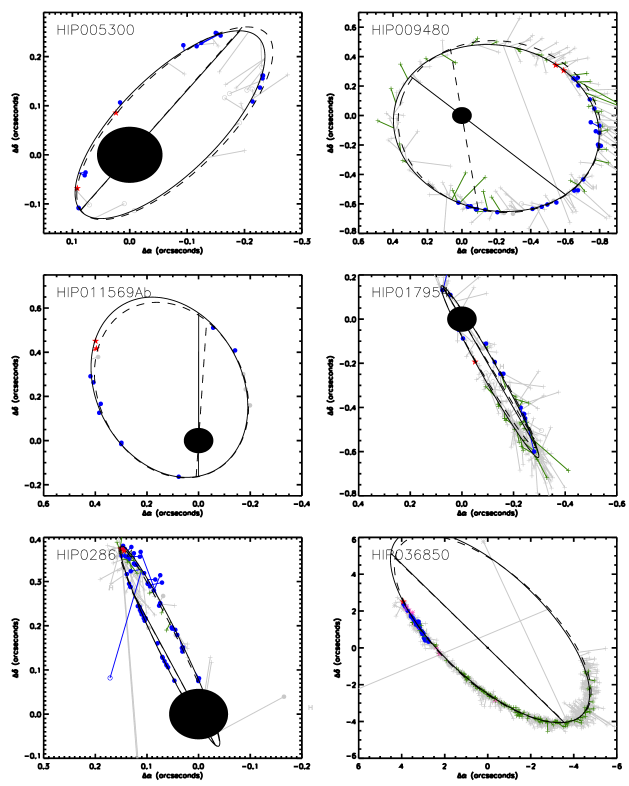
Figure 6: Combining our high resolution observations with historical measurements, refined orbits for 6 binary systems are plotted. The previous orbital fit, obtained from the Sixth Orbit Catalog, is plotted for reference with a dashed line. Each plot uses a similar symbol scheme to the Sixth Orbit Catalog; open blue circles representing eyepiece interferometry, filled blue circles speckle interferometry, green crosses micrometrical observations, and violet asterisks photographic measurements. Our high resolution observations presented within this study are plotted as filled red stars. For each measurement, the corresponding O-C line is plotted, showing the difference between expected and actual position within the orbital path. Symbols in grey represent those measurements presented without formal errors, and are not used while estimating the orbital parameters. Within each plot, the 57mas radius black disc represents the resolution limit for $K$-band observations at an 8-metre telescope.

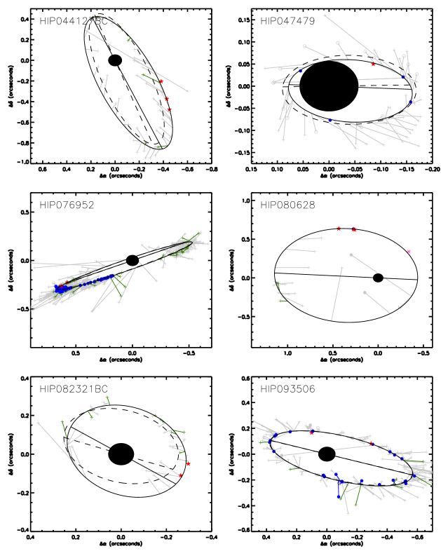
Figure 6: Combining our high resolution observations with historical measurements, refined orbits for 6 binary systems are plotted. The previous orbital fit, obtained from the Sixth Orbit Cataloge, is plotted for reference with a dashed line. Each plot uses a similar symbol scheme to the Sixth Orbit Catalog; open blue circles representing eyepiece interferometry, filled blue circles speckle interferometry, green crosses micrometrical observations, and violet asterisks photographic measurements. Our high resolution observations presented within this study are plotted as filled red stars. For each measurement, the corresponding O-C line is plotted, showing the difference between expected and actual position within the orbital path. Symbols in grey represent those measurements presented without formal errors, and are not used while estimating the orbital parameters. Within each plot, the 57mas radius black disc represents the resolution limit for $K$-band observations at an 8-metre telescope.

The orbital parameters for each system with sufficient orbital coverage are listed in Table LABEL:tab:orbits, alongside a system mass estimated from Kepler’s Third Law (hereafter the dynamical system mass) and the number of measurements used to fit the orbit. In Figure 6, the refined orbital fits incorporating the new data are plotted along with the previously reported orbit (references listed within Table 4). The resulting orbits span a range of periods from 10.78 to 467.4 years, and a range of semi-major axes between 0$\aas@@fstack{\prime\prime}$12 to 6$\aas@@fstack{\prime\prime}$78. The relatively short period of each system allows for orbital motion to be resolved over very short baselines, typically on the order of months. The changes to the estimated dynamical system mass between the previously published orbit fit and the refined fit presented within this study are shown in Table LABEL:tab:old_new_mass.

6 Discussion

Table 10: Comparison of dynamical and theoretical system masses for each system within the orbit subsample

	Dynamical		$\cdot$	Lejeune & Schaerer			$\cdot$	Marigo et al.			$\cdot$	Siess et al.
	System		$\cdot$	Age	System		$\cdot$	Age	System		$\cdot$	Age	System
HIP	Mass (M⊙)		$\cdot$	(Myr)	Mass (M⊙)		$\cdot$	(Myr)	Mass (M⊙)		$\cdot$	(Myr)	Mass (M⊙)
Systems identified as doubles (§6.1.1)
5300	3.16$\pm$	0.34	$\cdot$	280	3.56$\pm$	0.13	$\cdot$	400	3.47$\pm$	0.13	$\cdot$	355	3.69$\pm$	0.16
9480	2.72$\pm$	0.13	$\cdot$	250	3.15$\pm$	0.20	$\cdot$	280	3.12$\pm$	0.20	$\cdot$	160	3.25$\pm$	0.31
11569 AaAb†	2.12$\pm$	0.25	$\cdot$	100	2.45$\pm$	0.07	$\cdot$	100	2.89$\pm$	0.15	$\cdot$	100	2.97$\pm$	0.25
76952	4.19$\pm$	0.30	$\cdot$	315	4.38$\pm$	0.45	$\cdot$	400	4.10$\pm$	0.40	$\cdot$	315	4.38$\pm$	0.45
Low-mass binary pair within hierarchical system (§6.1.2, §6.1.3)
44127 BC	0.68$\pm$	0.04	$\cdot$	–	–		$\cdot$	250	0.88$\pm$	0.01	$\cdot$	50	0.83$\pm$	0.01
82321 BC	1.16$\pm$	0.09	$\cdot$	400	1.91$\pm$	0.02	$\cdot$	445	1.87$\pm$	0.02	$\cdot$	500	1.90$\pm$	0.02
Systems with one unresolved spectroscopic component (§6.2.1)
80628	4.99$\pm$	0.75	$\cdot$	630	3.03$\pm$	0.08	$\cdot$	630	3.06$\pm$	0.18	$\cdot$	445	3.15$\pm$	0.13
Systems with two unresolved spectroscopic components (§6.2.1)
28614	6.36$\pm$	0.62	$\cdot$	630	3.98$\pm$	0.32	$\cdot$	630	3.96$\pm$	0.28	$\cdot$	500	4.18$\pm$	0.34
36850	5.42$\pm$	0.97	$\cdot$	280	4.26$\pm$	0.28	$\cdot$	355	4.15$\pm$	0.24	$\cdot$	315	4.34$\pm$	0.31
Systems with evidence of unresolved spectroscopic components (§6.2.2)
17954	4.15$\pm$	0.39	$\cdot$	400	3.49$\pm$	0.11	$\cdot$	400	3.44$\pm$	0.12	$\cdot$	225	3.67$\pm$	0.16
47479	5.83$\pm$	0.53	$\cdot$	560	3.99$\pm$	0.10	$\cdot$	560	3.96$\pm$	0.10	$\cdot$	445	4.17$\pm$	0.14
93506	5.26$\pm$	0.37	$\cdot$	710	4.11$\pm$	0.25	$\cdot$	710	4.07$\pm$	0.23	$\cdot$	500	4.45$\pm$	0.36
† - The ages and theoretical masses may be significantly biased due to the presence of additional companions
within the resolution limit of the Tycho2 and 2MASS observations.

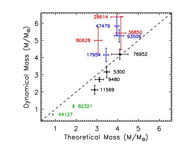
Figure 7: Using the method introduced in §4.4, a comparison can be made between the dynamical mass determined from the orbit and the mass estimated from theoretical mass-magnitude relations for the stars within the orbit subsample (the Marigo et al. (2008) models are used for this example). The systems with an A-type star primary which are known to consist only of two components are denoted as black points (§6.1.1). Two hierarchical systems were fully resolved with our data, and the lower-mass pair of each system are in green (§6.1.2). The systems which have a significantly discrepant dynamical mass can be explained by the presence of an unresolved spectroscopic companion within our data. The targets with known spectroscopic components are plotted in red (§6.2.1), while those systems with evidence suggesting a previously unknown spectroscopic component are plotted in blue (§6.2.2). The dashed line denotes the equivalence between the dynamical and theoretical mass.

We have presented high resolution observations obtained for 26 nearby multiple systems with A-type primaries with projected separations within 100 AU. The subset of 12 targets with orbit fits have been further divided into four distinct categories primarily based on a comparison between the dynamical mass and the theoretical mass estimated from the mass-magnitude relations, as shown in Figure 7. The theoretical mass estimates for each system using the Lejeune & Schaerer (2001), Marigo et al. (2008), and Siess et al. (2000) grids are shown in Table 10. Those systems with only two known components are discussed in §6.1.1, where the importance of metallicity is described. Two hierarchical systems resolved within our data are discussed in §6.1.2 and §6.1.3, which allow for a comparison to the models within the K- to M-type spectral range. For systems with a dynamical mass excess, significantly higher than the mass predicted from the theoretical mass-magnitude relations, the subset with known spectroscopic components is discussed in §6.2.1, and we present three systems with evidence suggestive of an additional unresolved component in §6.2.2. The remaining targets are discussed in the context of continued monitoring of the orbital motion in §6.3, of these 11 are newly resolved as a part of the VAST survey, 2 were resolved in recent multiplicity surveys of nearby Southern A-type stars (Ivanov et al., 2006; Ehrenreich et al., 2010), and 1 resolved within a large speckle interferometry survey (McAlister et al., 1987).

6.1 Comparison to theoretical models

6.1.1 A-type binaries

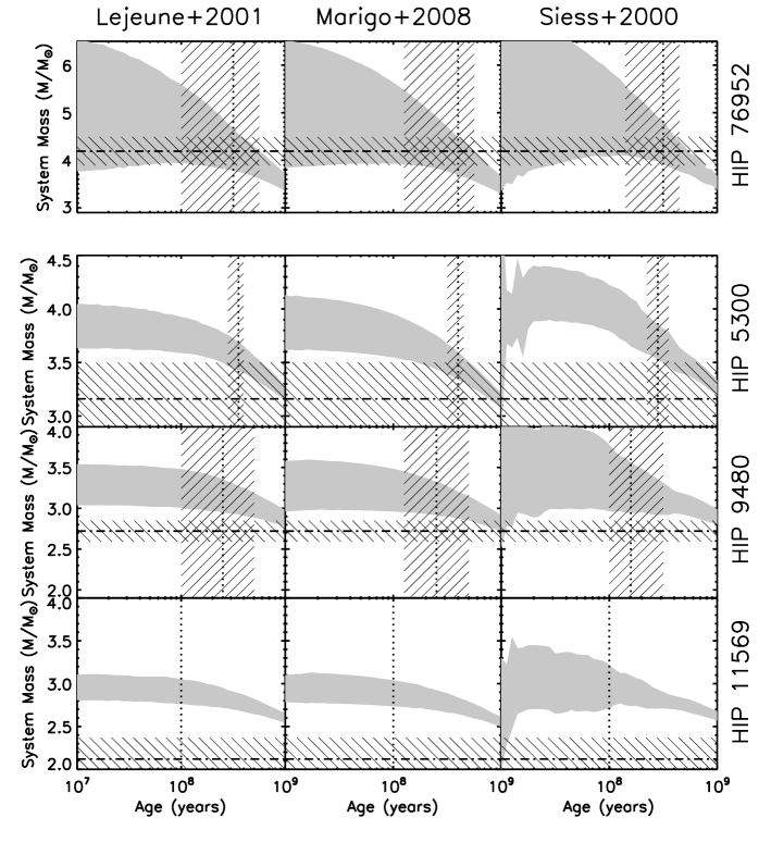
Figure 8: The system mass as a function of age based on the mass-magnitude relations derived from three of the model grids. Each panel is similar in nature to Figure 5, with the spread in the mass-age relation introduced by uncertainties in both the measured $K$-band magnitude, and the distance determination. The horizontal dot-dashed line indicates the dynamical mass determined from the system orbit, with the uncertainty denoted by the line-shaded region. The vertical dotted line indicates the age of the system derived from the isochrones, with the line-shaded region denoting the range of ages consistent with the uncertainties in the position of the primary on the CMD. The primary of the HIP 11569 system is significantly bluer than expected for a Main Sequence star, and as such its age has been assigned to 100 Myr, with no corresponding uncertainty. The presence of additional components to the HIP 11569 system, within the resolution limit of both the Tycho2 and 2MASS observations, is the likely cause of this bias.

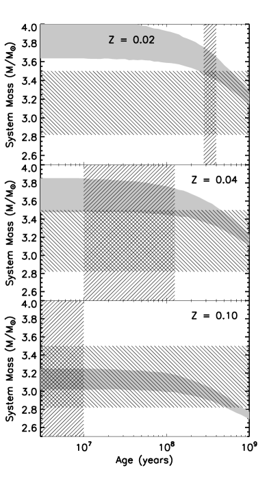
Figure 9: (top panel): The dynamical mass of the HIP 5300 system (horizontal line-shaded region) is significantly below that of the system mass estimated from mass-magnitude relations (solid shaded region) calculated from the Solar metallicity models from Lejeune & Schaerer (2001). (middle panel): Assuming a higher metallicity ($Z=0.04$), the position of the components on the colour-magnitude diagram suggests a younger age (denoted by the vertical line-shaded region), and the mass-magnitude relation derived from the metal-enhanced models suggests a systematically lower system mass, although the dynamical mass is still discrepant. (bottom panel): With a metallicity of $Z=0.10$, the age estimate is younger still ($<$10 Myr), and the discrepancy between the dynamical mass and the mass estimated from the mass-magnitude relation is removed.

Four targets within the orbit subsample are systems where the two known components have been resolved within our high resolution data; HIPs 5300, 9480, 11569, and 76952. For each of these four targets, the mass-magnitude relations were used to determine how the system mass changes as a function of our estimate of the system age, shown in Figure 8. For one system, HIP 76952, the dynamical system mass is consistent with the theoretical system mass (Figure 8, top panel). The ages of the systems estimated from the position of the primary on the CMD are consistent with their position within the Local Interstellar Bubble (LIB). The minimum age of a star within the LIB, excluding those with relatively high space motions (e.g. the $\beta$ Pic moving group - Ortega et al., 2002), has been shown to be 160 Myrs (Abt, 2011).

The dynamical system masses of the three remaining systems are consistently lower than their theoretical system masses. One possible explanation for the apparently low dynamical masses is a non-Solar metallicity. Varying the metallicity has a significant effect on the system age estimate and the mass-magnitude relations. As an example, a 2 M_⊙ star with super-Solar metallicity will be more luminous and have a redder $V-K$ colour index than a similar-mass star of Solar metallicity. A super-Solar metallicity star will appear to be significantly older based on its position on a CMD if Solar metallicity models are used. To explore the effect of our assumption of Solar metallicity for the entire sample, the HIP 5300 system (Figure 8, second panel) was studied at varying metallicity values. Using the Solar metallicity models, the dynamical system mass of this system is significantly lower than the theoretical system mass (Figure 9, top panel). Increasing the metallicity causes the star to appear both younger, and less massive (Figure 9, bottom panel). Only eight of the targets included within this study have metallicity measurements, either from spectroscopic analysis (e.g. Erspamer & North, 2003) or derived from Strömgren photometry (e.g. Song et al., 2001), demonstrating the need for further study in this area.

6.1.2 K- and M-type binaries - HIP 44127

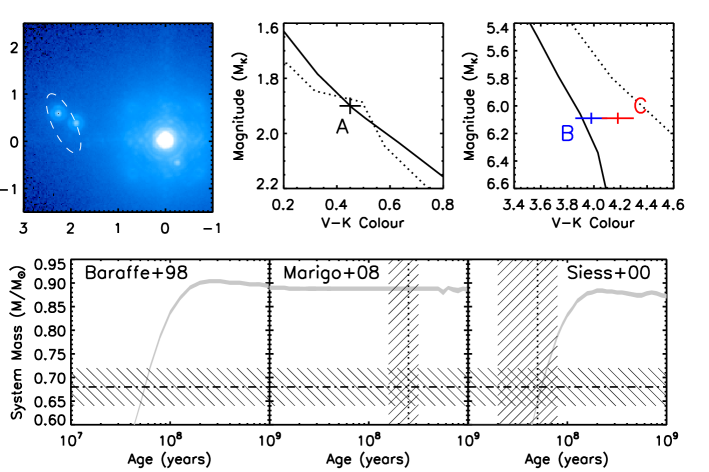
Figure 10: Top row - (left): An AO observation of HIP 44127 triple system. The orbit of the lower-mass pair (BC) taken from Table LABEL:tab:orbits is plotted as a solid line for reference. The bright point source to the lower-right of the primary PSF is a known filter ghost. The axis labels are given in arcseconds, with each arcsecond equal to approximately 14.5 AU. (centre): A colour-magnitude diagram highlighting the position of the primary with respect to the theoretical models; Marigo et al. (2008) - solid line, Siess et al. (2000) - dotted line, while the Baraffe et al. (1998) models do not extend to high enough masses. The age of the system was estimated using the isochrone which best fit the position of the primary. (right): A colour-magnitude diagram highlighting the position of the two lower-mass components (B - blue, C - red). The line styles are the same as the centre panel Bottom row - The theoretical system mass plotted as a function of system age for each of the three models. The vertical dotted line within each panel indicates the age of the system estimated from using each of the models, while the horizontal dot-dashed line indicates the dynamical system mass estimated from the orbital fit. As the Baraffe et al. (1998) models do not extend to the A-type star mass range, an age estimate is not possible.

The detection of two hierarchical systems, with pairs of lower-mass companions in a wide orbit around an A-type primary, allows for a comparison of the theoretical models in the low-mass regime where the models differ in the treatment of the contraction phase of these objects (e.g. Figure 3). Our observation of the HIP 44127 system, shown in Figure 10, resolves three components to this hierarchical system, with an A-star primary (A) separated by $\sim 4\arcsec$ from two fainter, gravitationally bound, companions (BC).

The orbit presented in the Sixth Orbit Catalog of the BC pair around the A-type primary is in disagreement with our recent observations of this system. Although the phase coverage is insufficient for a robust orbital determination, the high proper motion of the primary ($\Delta\alpha=-441.1$ mas yr^-1, $\Delta\delta=-215.2$ mas yr^-1) suggests that the BC pair is co-moving. In addition, radial velocity variations detected within the spectra of the primary suggest the presence of a spectroscopic component to this system with a period of $\sim$11 years (Abt, 1965). The separation of this component was anticipated to be between 0$\aas@@fstack{\prime\prime}$2 and 0$\aas@@fstack{\prime\prime}$6, reaching maximum separation in the middle of 2007 (Docobo & Andrade, 2006). We do not resolve any companion in any epoch of our observations which are consistent with these predictions, placing an upper limit to the separation of 0$\aas@@fstack{\prime\prime}$08, 0$\aas@@fstack{\prime\prime}$10, and 0$\aas@@fstack{\prime\prime}$10 in 2008, 2010, and 2011 respectively. The magnitude difference between the primary and the suggested companion, estimated to be $\Delta m=1.2$, is well within our detection limits at the expected separation (Docobo & Andrade, 2006).

A refined orbit of HIP 44127 BC is presented in Table LABEL:tab:orbits and Figure 6, with an estimated dynamical system mass of 0.68$\pm$0.04 M_⊙. The small magnitude difference between the two components ($\Delta K\sim 0$) suggests a mass ratio close to unity. Assuming individual masses of $\sim 0.34$ M_⊙ the components would be of early- to mid-M spectral type (Baraffe & Chabrier, 1996), a region of particular disagreement between theoretical models. The Baraffe et al. (1998) and Siess et al. (2000) models both predict that for a binary consisting of two stars of magnitudes equal to the measured magnitudes of the two components ($M_{K}=5.87$), the system mass will increase from 0.3 to 0.9 M_⊙ between 10 and 100 Myrs (Figure 10), as these models take into account the phase of contraction onto the Main Sequence for lower-mass stars. No such change is predicted by the Marigo et al. (2008) models, with the system mass remaining unchanged between 10 Myrs and 1 Gyr (Figure 10). The theoretical system masses are only consistent with the dynamical mass at $\sim 30$ Myrs in the Baraffe et al. (1998) and Siess et al. (2000) models, and are not consistent with any age in the Marigo et al. (2008) models. The metallicity of this system has been measured to be almost Solar (Wu et al., 2010), removing the degeneracy which exists between metallicity and the mass and age of the system (e.g. §6.2.6).

The position of the primary on the CMD suggests a relatively young age of the system between 50 and 250 Myr. The $V-K$ colours of the BC pair also suggest a young age, between 40 and 100 Myr using the Siess et al. (2000) and Baraffe et al. (1998) models. The inferred young age of the system is not inconsistent with the minimum age of stars found within the LIB (Abt, 2011), given the relatively high $UVW$ space velocity of the HIP 44127 system (Palous, 1983). The detection of X-ray emission from this system is also of interest. Previous studies have shown that A7 stars such as the primary should not emit X-rays, and that any detection of X-rays from the position of the star can be indicative of a lower-mass companion (e.g. De Rosa et al., 2011). The ROSAT source J085913.0+480227 is coincident with the optical position of HIP 44127 (Voges et al., 1999).

This hierarchical triple system warrants further study, primarily in order to refine the orbital fit as the BC pair approaches apastron passage in 2018. This system also makes an ideal candidate for future spectroscopic observations to search for the narrow spectral lines of the two faint companions. With a double-lined spectroscopic orbit fit, model-independent masses can be calculated for the individual components. If the young age suggested by both the position on the CMD and the system mass estimated from the mass-magnitude relations is correct, the BC pair would be an ideal calibrator for the theoretical models in the young, low-mass regime.

6.1.3 K- and M-type binaries - HIP 82321

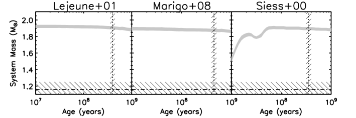
Figure 11: The theoretical system mass plotted as a function of system age for each of the three models for the HIP 82321 BC system. The vertical dotted line within each panel indicates the age of the system estimated from using each of the models, while the horizontal dot-dashed line indicates the dynamical system mass estimated from the orbital fit. The clear discrepancy between the dynamical and theoretical system masses can be explained by the lack of complete coverage of the orbit presented in Figure 6. Further high angular resolution observations of this system will allow for an improved determination of the orbital parameters.

The hierarchical triple system HIP 82321 was resolved within a single epoch of our AO observations. The A-type primary (A) is $\sim 2\arcsec$ from a binary pair of two lower-mass companions (BC) in a wide orbit. The significant proper motion of the primary ($\Delta\alpha=22.8$ mas yr^-1, $\Delta\delta=-51.4$ mas yr^-1), and near constant separation of the three stars, suggest that the lower-mass pair is co-moving with the primary. Spectroscopic measurements of the lower-mass components of this system are possible given the small magnitude difference of the pair with respect to the primary ($\Delta K\sim 2.5$); such spectra would allow for a determination of the individual masses independent of the distance to the system. The Hipparcos parallax and 2MASS $K$-band magnitude measurements of this system allow for a tight constraint of the system age to between 300 and 400Myrs, based on the position of the primary on the CMD. The primary is also a possible member of the Ursa Major moving group, an association of Solar metallicity stars with an age between 300 Myrs (Soderblom & Mayor, 1993) and 500 Myrs (King et al., 2003).

A refined orbit of the BC pair is presented in Table LABEL:tab:orbits, with an estimated dynamical system mass of 1.32$\pm$0.05 M_⊙. The theoretical system mass, assuming the distance to each component is the same as the primary, is significantly higher at $\sim 2.0$ M_⊙ (Figure 11). The sparse coverage of the orbit (Figure 6) suggests that the orbit fit could be poor, resulting in an incorrect dynamical system mass. The orbit fit would be significantly improved with subsequent observations. An alternative scenario is that the pair are a background binary with a proper motion similar to the primary, which would bring the dynamical and photometrically derived masses into agreement.

6.2 Higher-order multiplicity

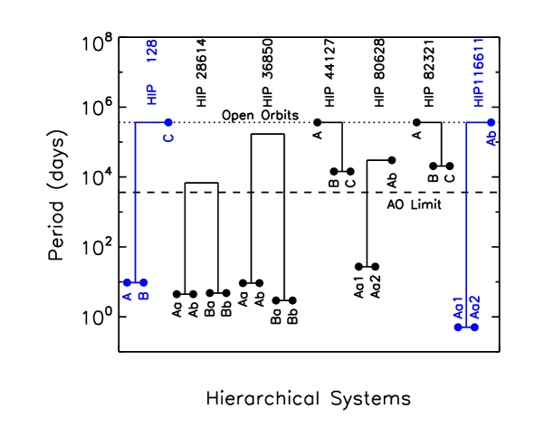
Figure 12: A schematic of the 7 hierarchical systems within both subsamples, including only components within a projected separation of 100AU to the A-type primary. The schematic diagram does not include the suspected spectroscopic binaries described in §6.2.2. Those systems which were newly resolved as a part of the VAST survey are highlighted in blue. Each filled circle represents an individual component, with the period of the binary pair denoted by its vertical position. Our high resolution observations are only sensitive to systems with orbital periods greater than $\sim$ 10 years, denoted by the dashed horizontal line. For wide separation systems with indeterminate orbital periods, such as HIP 128 AB–C, the orbital period has been arbitrarily set at 1000 years, denoted by the dotted horizontal line.

6.2.1 Known spectroscopic binaries

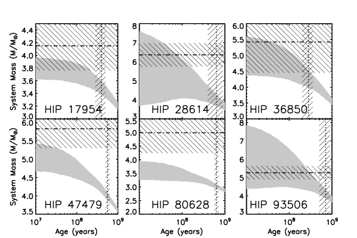
Figure 13: The six systems for which spectroscopic components are either known to be present through previous spectroscopic observations (HIPs 28614, 36850, 80628), or thought to exist due to a significant discrepancy between the theoretical system mass and the dynamical system mass. For clarity only one model has been used to estimate the theoretical system mass (Lejeune & Schaerer, 2001). The horizontal displacement between the intersection of the dynamical system mass (dot-dashed line) and the age estimate of the system (dotted line), and the theoretical system mass curve (solid shaded region), gives an order of magnitude estimate of the mass of the unresolved spectroscopic components.

The presence of an unresolved spectroscopic binary can have a significant impact on the magnitude assigned to each component of the multiple system, increasing the estimated component magnitude by as much as 0.75 mag for an unresolved equal-mass spectroscopic binary. For each target within this study, the literature was searched for references to additional components resolved through spectroscopic or interferometric observation which would influence any comparison made between the dynamical system mass and the theoretical system mass (e.g. Figure 13). Of the targets within the orbit subsample, three are known to have additional spectroscopic components (HIPs 28614, 36850, 80628). The spectroscopic component to HIP 9480 resolved by Abt (1965) is resolved within our adaptive optics observations. Similarly, for the monitoring subsample, two are known spectroscopic binaries (HIPs 128, 116611). The greater frequency of spectroscopic binaries within the orbit sample, relative to the monitoring sample, can be explained by the narrow spectral lines of the former sample due to their relatively low radial velocities, $\langle v\sin i\rangle=71$ km s^-1 compared with $\langle v\sin i\rangle=115$ km s^-1 for the latter sample (Abt & Morrell, 1995). The magnitudes listed for the resolved components of these systems (Table 6) are the blended magnitudes of the listed spectroscopic components. In addition to these known spectroscopic binaries, three members of the orbit subsample are resolved as hierarchical triples within our high resolution observations (HIPs 11569, 44128, 82321). A schematic representation of the higher-order multiplicity systems is given in Figure 12.

For the three systems with known spectroscopic components within the orbit sample, the dynamical system mass includes the mass of each component, regardless of whether it is resolved within our data. This causes a significant discrepancy when the dynamical system mass is compared with the theoretical system mass (e.g. Figure 7), with the dynamical system mass being systematically higher. The discrepancy between the two values cannot be directly converted into a mass for the unresolved components however, as a blended magnitude would have been used when determining the mass from the mass-magnitude relations.

6.2.2 Evidence of spectroscopic components

Systems with significantly higher dynamical masses than theoretical masses obtained from mass-magnitude relations are strong candidates for multiple systems with unresolved components which have not been detected in spectroscopic observations. We find two such systems with the signature of a possible unresolved component: HIP 17954 and HIP 93506 (Figure 13), with masses of the order of 0.5 and 1.5 M_⊙. Sensitive spectroscopic observations of both systems may lead to the detection of the spectral lines from an unresolved lower-mass component. A similar phenomenon is observed for the HIP 47479 system, although the number of measurements used to determine the orbit is particularly low, making the dynamical mass less certain. The narrow spectral lines of HIP 47479, implied by the low measured stellar rotational velocity (Royer et al., 2007), make it an ideal candidate for spectroscopic follow up. Previous spectroscopic observations of this system reveal $v\sin i$ variations with a magnitude of 40 km s^-1 (Moore, 1932).

From the total sample of 26 systems, and only considering stellar companions within 100 AU, a lower-limit on the higher-order multiplicity of A-type stars can be estimated. Assuming the suspected unresolved companions described earlier in this section are true, there are five double, six triple, and two quadruple systems within the orbit subsample, corresponding to frequencies of 39, 46, and 15 per cent, respectively. This lower-limit shows an enhancement on the higher-order multiplicity of A-type stars when compared with Solar-type primaries (74 per cent double, 20 per cent triple, and 6 per cent quadruple or higher-order - Raghavan et al., 2010), and is more consistent with the fraction reported for more massive O-type primaries (46 per cent double, and 54 per cent triple or higher-order - Mason et al., 2009).

6.3 Continued monitoring targets

6.3.1 Newly-resolved binaries

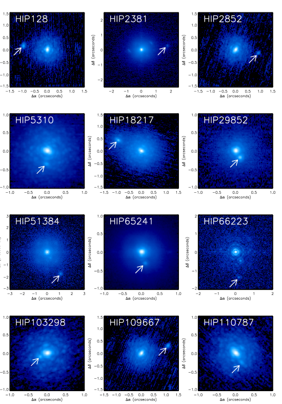
Figure 14: Observations of twelve of the thirteen systems with projected separations $<100$AU suggested as future orbital monitoring targets. The companion in each image is highlighted, with a logarithmic image scale between $1$ (white) and $10^{-6}$ (black) relative to the peak intensity of the primary.

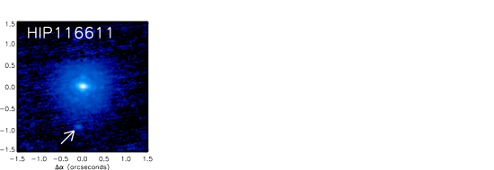
Figure 14: (continued): An observation of one of the thirteen systems with projected separations $<100$AU suggested as future orbital monitoring targets. The companion in each image is highlighted, with a logarithmic image scale between $1$ (white) and $10^{-6}$ (black) relative to the peak intensity of the primary.

We have identified 13 binary systems with projected separations ranging between 13 AU and 96 AU which would make ideal candidates for future orbital monitoring projects (Table 5). The 100 AU projected separation cut-off was applied to select only systems for which orbital motion could be detected with several years of observations. The binaries resolved within the monitoring subsample typically have lower-mass ratios than for the orbit subsample, a demonstration of the effectiveness of AO observations at detecting high-contrast binaries. Based on their position on the CMD, two members of the monitoring subsample (HIP 5310, HIP 18217) appear to lie on the Zero-Age Main Sequence, and the measured magnitude difference between primary and secondary would correspond to a late K or early M-type companion in each case. These companions are of particular interest as they will allow for further tests of the theoretical models within the young, low-mass regime. A gallery of the observations obtained of each target within the monitoring subsample is shown in Figure14.

6.3.2 HIP 77660

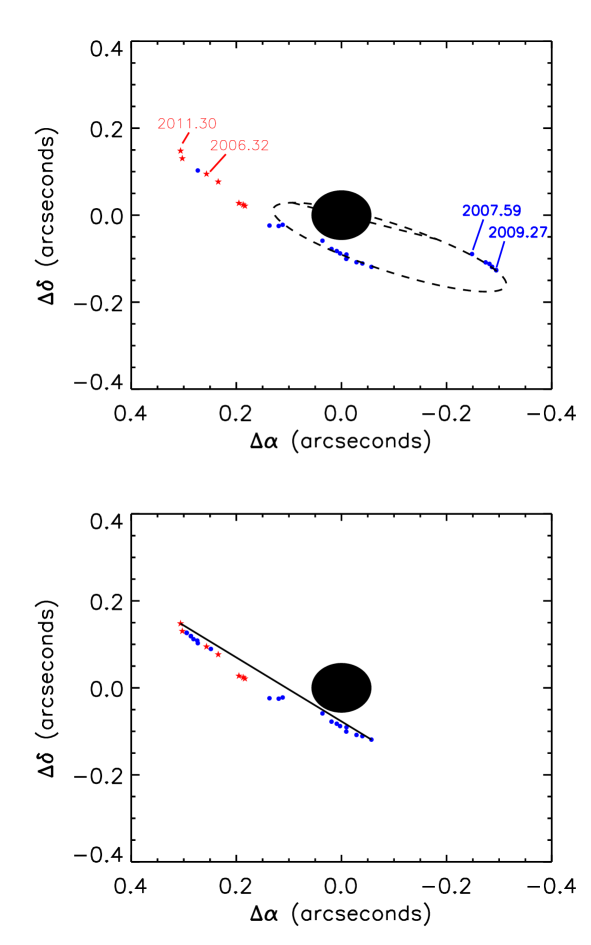
Figure 15: (top panel): The historical measurement of the system HIP 77660, plotted with the orbital fit estimated by Docobo et al. (2010). This system demonstrates the quadrant ambiguity limitation of the speckle interferometry technique. The binary companion was measured by Tokovinin et al. (2010) using speckle interferometry to be at a position angle of 248.4^∘ to 246.8^∘ between mid-2007 and mid-2009 (blue filled circles, top right). Our AO images, which do not suffer from the same quadrant ambiguity, shows the binary at a position angle of 69.7^∘ to 67.3^∘ between mid-2006 and mid-2011 (red filled stars, left). (bottom panel): The relative position of the secondary, with 180^∘ added to the four speckle interferometry measurements which were inconsistent with the observations presented within this study. The solid line connects the first and last observations, showing a deviation away from linear motion. Further observations are required to determine if this deviation is indicative of the true orbital path of the secondary about the primary.

An advantage of monitoring binary systems for orbital motion with AO instrumentation over interferometric techniques is the elimination of the quadrant ambiguity. In some cases, the output of the image processing of speckle data results in a 180^∘ ambiguity on the position angle measurement (Bagnuolo et al., 1992). This may lead to a scenario where orbital motion is thought to exist for a binary pair, when in fact this motion is the product of such a quadrant uncertainty combined with the true linear motion of the companion. The ambiguity can be resolved by observing the system using AO imaging, where no reconstruction is required to obtain the final science image.

Based on our AO observations of the binary system HIP 77660, it appears that such a quadrant ambiguity has occurred, making linear motion appear as orbital motion, as shown in Figure 15. The significant proper motion of the system ($\Delta\alpha=-91$ mas/yr, $\Delta\delta=-28$ mas/yr), as measured by Hipparcos, is inconsistent with a stationary background object. While future measurements of this system will be able to resolve the presence of orbital motion after a sufficient time baseline, spectroscopy or multi-colour photometry will allow for a rapid characterisation of the properties of both components.

7 Summary

We have presented high resolution observations of 26 nearby multiple systems with A-type primaries with projected separations $<$ 100 AU, 11 of which are binaries newly resolved as a part of the VAST survey. For those systems with sufficient orbital motion coverage, refined orbital parameters were calculated and the estimated dynamical system mass was compared to masses derived from theoretical models. Due to their rapid evolution across the CMD, removing the significant age degeneracy for lower-mass solar-type stars, binaries with A-type components are ideal targets with which to test theoretical models. Four such systems were investigated, with one system having consistent dynamical and theoretical system mass estimates. Of the remaining three systems, each had a dynamical mass significantly lower than that predicted from the models. While this discrepancy may be indicative of a true divergence between the models and observations, the lack of metallicity measurements for these systems provide another explanation. Future orbital monitoring observations of A-star binary systems will provide further refinement to the orbital parameters and, combined with refinement of the magnitude, metallicity, and parallax measurements, will improve the analysis performed within this study.

Observations of two hierarchical systems, consisting of an A-type primary and a tight low-mass binary pair in a wide orbit allowed us to extend this analysis to the lower mass regime. The primary of the triple HIP 44127 suggests a young system age ($<$100 Myr), making the M-dwarf pair interesting for comparison with evolutionary models. We have also shown that a dynamical system mass significantly higher than the theoretical system mass is suggestive of an unresolved spectroscopic component within the system. Demonstrated on several known spectroscopic binaries, systems which exhibit this discrepancy are ideal candidates for future spectroscopic or interferometric observations in an attempt to detect these hypothetical companions. Interferometric observations may be required to resolve these purported companions, as the rotationally broadened spectral lines of the rapidly rotating members of the monitoring sample (Abt & Morrell, 1995) may preclude the detection of additional components using spectroscopy. Including the three systems with evidence of an unresolved close companion, a lower-limit on the higher-order multiplicity can be estimated from the 13 systems within the orbit subsample as 39 per cent double, 46 per cent triple, and 15 per cent quadruple. The frequency of single A-type stars will be explored in an upcoming publication within the VAST survey paper series. The remaining systems for which an orbit could not be determined are candidates for orbital monitoring projects with ground-based high resolution observations. A number of these systems are of particular interest, based on age estimates derived from the position of the primary on the CMD, and the magnitude difference between the two components.

References

- Abt (1965) Abt H. A., 1965, ApJS, 11, 429
- Abt (2011) Abt H. A., 2011, AJ, 141, 165
- Abt & Morrell (1995) Abt H. A., Morrell N. I., 1995, ApJS, 99, 135
- Andersen et al. (1991) Andersen J., Clausen J. V., Nordstrom B., Tomkin J., Mayor M., 1991, A&A, 246, 99
- Bagnuolo et al. (1992) Bagnuolo W. G. J., Mason B. D., Barry D. J., Hartkopf W. I., McAlister H. A., 1992, AJ, 103, 1399
- Baize & Petit (1989) Baize P., Petit M., 1989, A&AS, 77, 497
- Baraffe & Chabrier (1996) Baraffe I., Chabrier G., 1996, ApJ, 461, L51
- Baraffe et al. (1998) Baraffe I., Chabrier G., Allard F., Hauschildt P. H., 1998, A&A, 337, 403
- Bate (2000) Bate M. R., 2000, MNRAS, 314, 33
- Bonnefoy et al. (2009) Bonnefoy M., Chauvin G., Dumas C., Lagrange A.-M., Beust H., Desort M., Teixeira R., Ducourant C., Beuzit J.-L., Song I., 2009, A&A, 506, 799
- Bonnell (2001) Bonnell I. A., 2001, The Formation of Binary Stars, 200, 23
- Carpenter (2001) Carpenter J. M., 2001, AJ, 121, 2851
- Carquillat et al. (2003) Carquillat J.-M., Ginestet N., Prieur J. L., Debernardi Y., 2003, MNRAS, 346, 555
- Christou & Drummond (2006) Christou J. C., Drummond J. D., 2006, AJ, 131, 3100
- De Rosa et al. (2011) De Rosa R. J., Bulger J., Patience J., Leland B., Macintosh B., Schneider A., Song I., Marois C., Graham J. R., Bessell M., Doyon R., 2011, MNRAS, 415, 854
- Docobo & Andrade (2006) Docobo J. A., Andrade M., 2006, ApJ, 652, 681
- Docobo & Costa (1985) Docobo J. A., Costa J. M., 1985, Circ. d’Inf., 96
- Docobo & Ling (2007) Docobo J. A., Ling J. F., 2007, AJ, 133, 1209
- Docobo et al. (2010) Docobo J. A., Tamazian V. S., Balega Y. Y., Melikian N. D., 2010, AJ, 140, 1078
- Doyon et al. (1998) Doyon R., Nadeau D., Vallee P., Starr B. M., Cuillandre J. C., Beuzit J.-L., Beigbeder F., Brau-Nogue S., 1998, SPIE, 3354, 760
- Drummond et al. (2003) Drummond J., Milster S., Ryan P., Roberts Jr L. C., 2003, ApJ, 585, 1007
- Ducati (2002) Ducati J. R., , 2002, Stellar Photometry in Johnson’s 11-Color System (Strasbourg: CDS)
- Dupuy et al. (2009) Dupuy T. J., Liu M. C., Bowler B. P., 2009, ApJ, 706, 328
- Eggen (1967) Eggen O. J., 1967, ARA&A, 5, 105
- Ehrenreich et al. (2010) Ehrenreich D., Lagrange A.-M., Montagnier G., Chauvin G., Galland F., Beuzit J.-L., Rameau J., 2010, A&A, 523, 73
- Erspamer & North (2003) Erspamer D., North P., 2003, A&A, 398, 1121
- ESA (1997) ESA 1997, The Hipparcos and Tycho Catalogues, ESA SP-1200
- Fabricius & Makarov (2000) Fabricius C., Makarov V. V., 2000, A&A, 356, 141
- Fekel et al. (2002) Fekel F. C., Scarfe C. D., Barlow D. J., Hartkopf W. I., Mason B. D., McAlister H. A., 2002, AJ, 123, 1723
- Green (1985) Green R. M., 1985, Cambridge and New York, Cambridge University Press, 1985, 533 p.
- Gutmann (1965) Gutmann F., 1965, Publications of the Dominion Astrophysical Observatory Victoria, 12, 391
- Hartkopf et al. (1989) Hartkopf W. I., McAlister H. A., Franz O. G., 1989, AJ, 98, 1014
- Hartkopf et al. (2012) Hartkopf W. I., Tokovinin A., Mason B. D., 2012, AJ, 143, 42
- Hayward et al. (2001) Hayward T. L., Brandl B., Pirger B., Blacken C., Gull G. E., Schoenwald J., Houck J. R., 2001, PASP, 113, 105
- Hilditch (2001) Hilditch R. W., 2001, An Introduction to Close Binary Stars
- Hodapp et al. (2003) Hodapp K. W., Jensen J. B., Irwin E. M., Yamada H., Chung R., Fletcher K., Robertson L., Hora J. L., Simons D. A., Mays W., Nolan R., Bec M., Merrill M., Fowler A. M., 2003, PASP, 115, 1388
- Horch et al. (2001) Horch E., Ninkov Z., Franz O. G., 2001, AJ, 121, 1583
- Horch et al. (2004) Horch E. P., Meyer R. D., van Altena W. F., 2004, AJ, 127, 1727
- Ivanov et al. (2006) Ivanov V. D., Chauvin G., Foellmi C., Hartung M., Huélamo N., Melo C., Nürnberger D., Sterzik M., 2006, Ap&SS, 304, 247
- King et al. (2003) King J. R., Villarreal A. R., Soderblom D. R., Gulliver A. F., Adelman S. J., 2003, AJ, 125, 1980
- Köhler et al. (2008) Köhler R., Ratzka T., Herbst T. M., Kasper M., 2008, A&A, 482, 929
- Kratter et al. (2010) Kratter K. M., Murray-Clay R. A., Youdin A. N., 2010, ApJ, 710, 1375
- Lejeune & Schaerer (2001) Lejeune T., Schaerer D., 2001, A&A, 366, 538
- Lenzen et al. (2003) Lenzen R., Hartung M., Brandner W., Finger G., Hubin N. N., Lacombe F., Lagrange A.-M., Lehnert M. D., Moorwood A. F. M., Mouillet D., 2003, SPIE, 4841, 944
- Liu et al. (2008) Liu M. C., Dupuy T. J., Ireland M. J., 2008, ApJ, 689, 436
- Lloyd et al. (2000) Lloyd J. P., Liu M. C., Macintosh B. A., Severson S. A., Deich W. T., Graham J. R., 2000, SPIE, 4008, 814
- Lodato et al. (2007) Lodato G., Meru F., Clarke C. J., Rice W. K. M., 2007, MNRAS, 374, 590
- McAlister et al. (1987) McAlister H. A., Hartkopf W. I., Hutter D. J., Franz O. G., 1987, AJ, 93, 688
- McCaughrean & Stauffer (1994) McCaughrean M. J., Stauffer J. R., 1994, AJ, 108, 1382
- McDonald & Clarke (1995) McDonald J. M., Clarke C. J., 1995, MNRAS, 275, 671
- Marigo et al. (2008) Marigo P., Girardi L., Bressan A., Groenewegen M. A. T., Silva L., Granato G. L., 2008, A&A, 482, 883
- Mason et al. (1999) Mason B. D., Douglass G. G., Hartkopf W. I., 1999, AJ, 117, 1023
- Mason et al. (2009) Mason B. D., Hartkopf W. I., Gies D. R., Henry T. J., Helsel J. W., 2009, AJ, 137, 3358
- Mason et al. (2001) Mason B. D., Wycoff G. L., Hartkopf W. I., Douglass G. G., Worley C. E., 2001, AJ, 122, 3466
- Moore (1932) Moore J. H., 1932, Publications of Lick Observatory, 18, 1
- Morel & Magnenat (1978) Morel M., Magnenat P., 1978, A&AS, 34, 477
- Muterspaugh et al. (2010) Muterspaugh M. W., Hartkopf W. I., Lane B. F., O’Connell J., Williamson M., Kulkarni S. R., Konacki M., Burke B. F., Colavita M. M., Shao M., Wiktorowicz S. J., 2010, AJ, 140, 1623
- Muterspaugh et al. (2008) Muterspaugh M. W., Lane B. F., Fekel F. C., Konacki M., Burke B. F., Kulkarni S. R., Colavita M. M., Shao M., Wiktorowicz S. J., 2008, AJ, 135, 766
- Ortega et al. (2002) Ortega V. G., de la Reza R., Jilinski E., Bazzanella B., 2002, ApJ, 575, L75
- Palous (1983) Palous J., 1983, Bulletin of the Astronomical Institutes of Czechoslovakia, 34, 286
- Popovic (1969) Popovic G. M., 1969, Bulletin de l’Observatoire Astronomique de Belgrade, 27, 33
- Press et al. (1992) Press W. H., Teukolsky S. A., Vetterling W. T., Flannery B. P., 1992, Cambridge: University Press, —c1992, 2nd ed.
- Pringle (1989) Pringle J. E., 1989, MNRAS, 239, 361
- Raghavan et al. (2010) Raghavan D., McAlister H. A., Henry T. J., Latham D. W., Marcy G. W., Mason B. D., Gies D. R., White R. J., ten Brummelaar T. A., 2010, ApJS, 190, 1
- Rousset et al. (2003) Rousset G., Lacombe F., Puget P., Hubin N. N., Gendron E., Fusco T., Arsenault R., Charton J., Feautrier P., Gigan P., Kern P. Y., Lagrange A.-M., Madec P.-Y., Mouillet D., Rabaud D., Rabou P., Stadler E., Zins G., 2003, SPIE, 4839, 140
- Royer et al. (2007) Royer F., Zorec J., Gómez A. E., 2007, A&A, 463, 671
- Rucinski et al. (2005) Rucinski S. M., Pych W., Ogłoza W., DeBond H., Thomson J. R., Mochnacki S. W., Capobianco C. C., Conidis G., Rogoziecki P., 2005, AJ, 130, 767
- Siess et al. (2000) Siess L., Dufour E., Forestini M., 2000, A&A, 358, 593
- Skrutskie et al. (2006) Skrutskie M. F., Cutri R. M., Stiening R., Weinberg M. D., Schneider S., Carpenter J. M., Beichman C., Capps R., Chester T., Elias J., Huchra J., Liebert J., Lonsdale C., Monet D. G., Price S., Seitzer P., 2006, AJ, 131, 1163
- Soderblom & Mayor (1993) Soderblom D. R., Mayor M., 1993, AJ, 105, 226
- Söderhjelm (1999) Söderhjelm S., 1999, A&A, 341, 121
- Song et al. (2001) Song I., Caillault J.-P., Navascues D. B. y., Stauffer J. R., 2001, ApJ, 546, 352
- Stamatellos et al. (2007) Stamatellos D., Hubber D. A., Whitworth A. P., 2007, MNRAS, 382, L30
- Stassun et al. (2008) Stassun K. G., Mathieu R. D., Cargile P. A., Aarnio A. N., Stempels E., Geller A., 2008, Nature, 453, 1079
- Tokovinin (2008) Tokovinin A., 2008, MNRAS, 389, 925
- Tokovinin et al. (2010) Tokovinin A., Mason B. D., Hartkopf W. I., 2010, AJ, 139, 743
- van Leeuwen (2007) van Leeuwen F., 2007, A&A, 474, 653