On a continuous mixed strategies model for evolutionary game theory

Abstract

We consider an integro-differential model for evolutionary game theory which describes the evolution of a population adopting mixed strategies. Using a reformulation based on the first moments of the solution, we prove some analytical properties of the model and global estimates. The asymptotic behavior and the stability of solutions in the case of two strategies is analyzed in details. Numerical schemes for two and three strategies which are able to capture the correct equilibrium states are also proposed together with several numerical examples.

Key words. Continuous mixed strategies, Replicator dynamics, Evolutionary Game Theory, Kinetic equations, Numerical methods.

1 Introduction

Evolutionary dynamics is based on the ideas of mathematical game theory. In game theory, a player’s strategy in a game is a complete plan of action at any stage of the game. A pure strategy defines a specific move or action that a player will follow in every possible attainable situation in a game. A player’s strategy set is the set of pure strategies available to that player and defines what strategies are available to play. A mixed strategy is an assignment of a probability to each pure strategy. This allows for a player to select a pure strategy with a given distribution of probability. Since probabilities are continuous, there are infinitely many mixed strategies available to a player, even if their strategy set is finite. Of course, one can regard a pure strategy as a degenerate case of a mixed strategy, in which that particular pure strategy is selected with probability $1$ and every other strategy with probability $0$.

In any game, an important concept is the payoff that is the number which represents the motivations of a player. The exact definition of the payoff depends on the case of interest: payoff may represent profit, utility, or other continuous measures, or may simply rank the desirability of outcomes. In all cases, the payoffs must reflect the motivations of the players. Following the basic tenet of Darwinism, we may express the success of a player in a game, that means the player’s survival, as the difference between the player’s payoff and the average payoff of all players.

Dynamic models for continuous strategy spaces have received considerable attention recently both in theoretical biology when considering the evolution of species traits [1, 5, 9] and in economy when predicting rational behavior of individuals whose payoffs are given through game interactions [3, 6].

In the present paper we analyze a continuous mixed strategies model for population dynamics based on an integro-differential representation. Analogous models based on the replicator equation with continuous strategy space were recently investigated in [2, 4, 10, 12, 13]. In contrast with finite strategy spaces, where the notion of equilibrium is well understood and studied [11, 15], the situation of games with infinite strategies is still missing a general theory due to several technical and conceptual difficulties [12].

The model here considered is characterized by a continuous density function $f(t,\bf q)$ of population adopting the $\bf q\in\mathbb{R}^{N}$ strategy at time $t$ and presents some analogies with classical kinetic or mean field approaches. In particular we show that the model, which contains a cubic nonlinearity in $f$, can be reformulated in terms of the first moments of the solution. Such reformulation is essential in our analysis and in the derivation of numerical approximations.

For the moment based model we prove global existence of solutions and study the asymptotic behavior and stability of solutions in the case of two strategies. Two classes of stationary solutions are found. Continuous stationary solutions are characterized by every density function with a given mean strategy. If we consider more general solutions, so that the probability distributions are no more absolutely continuous with respect to the Lebesgue measure, another class of stationary solutions is given by concentrated Dirac masses. Numerical schemes for the two and three strategy case which are able to capture the correct equilibrium states are also proposed together with several numerical examples.

The rest of the paper is organized as follows. In Section 2, we present the model for $N$ pure strategies and prove a priori estimates and the global existence of solutions. In Section 3, we put the emphasis on the model with two pure strategies, which can be reduced to a 1D model, and study the asymptotic behavior of the solutions and their relation with stationary solutions. Section 4 is dedicated to the numerical approximation of the 1D model and to numerical tests for the Prisoner’s Dilemma and for the Hawk or Dove games, with results about the a priori estimate, the asymptotic behavior of the solutions and the stationary solutions. In Section 5 and 6, we present the 2D model and the numerical tests for the Rock-Scissors-Paper game. Some final considerations are reported in the last section.

2 An integro-differential model for continuous mixed strategies

2.1 Setting of the model

First, we introduce an integro-differential model for continuous mixed strategies. We start from some preliminary concepts and definitions taken from [11]. Assume that we have a game where there are $N$ pure strategies $R_{1}$ to $R_{N}$ and that the players can use mixed strategies: these consists in playing the pure strategies $R_{1}$ to $R_{N}$ with some probabilities $q_{1}$ to $q_{N}$ with $q_{i}\geq 0$ and $\sum q_{i}=1$. A strategy corresponds to a point ${\bf{q}}$ in the simplex

$$\mathcal{S}_{N}:=\displaystyle\{{\bf{q}}=(q_{1},\dots,q_{N})\in\mathbb{R}^{N}:q_{i}\geq 0\mbox{ and }\displaystyle\sum_{i=1}^{N}q_{i}=1\}.$$ (1)

The corners of the simplex are the standard unit vectors ${\bf{e}}_{i}$ with the $i$-th component is $1$ and all others are $0$ and correspond to the $N$ pure strategies $R_{i}$, $i=1,\dots,N$.

Let us denote by $a_{ij}$ the payoff for a player using the pure strategy $R_{i}$ against a player using the pure strategy $R_{j}$. The $N\times N$ matrix $\mathcal{A}=(a_{ij})$ is said to be the payoff matrix. An $R_{i}$-strategist obtains the expected payoff $(\mathcal{A}{\bf{q^{*}}})_{i}=\sum_{j}a_{ij}q^{*}_{j}$ against a ${\bf{q^{*}}}$-strategist, since $q^{*}_{j}$ is the probability that he is met with strategy $R_{j}$. The payoff for a ${\bf{q}}$-strategist against a ${\bf{q^{*}}}$-strategist is given by

$$A({\bf{q}},{\bf{q^{*}}}):={\bf{q}}\cdot\mathcal{A}{\bf{q^{*}}}=\sum_{i,j=1}^{N}a_{ij}q_{i}q^{*}_{j}.$$ (2)

We consider a population of individuals as a player of the game and denote by $f(t,{\bf{q}})$ the density of population adopting the ${\bf{q}}$ strategy at time $t$; the evolution in time of $f$, due to the dynamics of the game, is driven by

$$\partial_{t}f(t,{\bf{q}})=f(t,{\bf{q}})\,\left(\int_{\mathcal{S}_{N}}A({\bf{q}},{\bf{q^{*}}})f(t,{\bf{q^{*}}})\,d{\bf{q^{*}}}-\phi(f)\right),$$ (3)

where the term

$$\int_{\mathcal{S}_{N}}A({\bf{q}},{\bf{q^{*}}})f(t,{\bf{q^{*}}})\,d{\bf{q^{*}}}$$ (4)

represents the payoff of the strategy ${\bf{q}}$ against all the others strategies, $A({\bf{q}},{\bf{q^{*}}})$ being the interacting kernel between the ${\bf{q}}$-strategist and the ${\bf{q^{*}}}$-strategist. The last term of the equation (7) is defined by

$$\phi(f):=\int_{\mathcal{S}_{N}}\,\int_{\mathcal{S}_{N}}f(t,{\bf{q}})\,A({\bf{q}},{\bf{q^{*}}})\,f(t,{\bf{q^{*}}})\,d{\bf{q^{*}}}\,d{\bf{q}}$$ (5)

and represents the average payoff of the population.

Since $\sum_{i=1}^{N}q_{i}=1,$ we can reduce the number of variables, considering

$$q_{N}=1-\sum_{i=1}^{N-1}q_{i}$$

and obtaining the $(N-1)$ - dimensional model (3), on the simplex

$$\mathcal{T}_{N-1}:=\{{\bf{p}}=(p_{1},p_{2},\dots,p_{N-1})\in\mathbb{R}^{N-1}\,|\,p_{i}\geq 0\,,\sum_{i=1}^{N-1}p_{i}\leq 1\},$$ (6)

namely

$$\partial_{t}f(t,{\bf{p}})=f(t,{\bf{p}})\,\left(\int_{\mathcal{T}_{N-1}}A({\bf{p}},{\bf{p^{*}}})f(t,{\bf{p^{*}}})\,d{\bf{p^{*}}}-\phi(f)\right),$$ (7)

with $A({\bf{p}},{\bf{p^{*}}})$ defined by

$$A({\bf{p}},{\bf{p^{*}}}):={\bf{p}}\cdot\mathcal{A}{\bf{p^{*}}}=\sum_{i,j=1}^{N-1}a_{ij}p_{i}p^{*}_{j},$$ (8)

and $\phi$ defined by

$$\phi(f):=\int_{\mathcal{T}_{N-1}}\,\int_{\mathcal{T}_{N-1}}f(t,{\bf{p}})\,A({\bf{p}},{\bf{p^{*}}})\,f(t,{\bf{p^{*}}})\,d{\bf{p^{*}}}\,d{\bf{p}}.\\$$ (9)

Remark 1.

If we take an initial condition

$$f(0,{\bf{p}})=f_{0}({\bf{p}})\geq 0,$$ (10)

with $\int_{\mathcal{T}_{N-1}}f_{0}({\bf{p}})d{\bf{p}}=1$, then it is easy to see that $f\geq 0$ for all $t>0$ and if $f_{0}({\bf{\bar{p}}})=0$ for some ${\bf{\bar{p}}}$, then $f(t,{\bf{\bar{p}}})=0$ for all $t>0$. We have also that

$$\int_{\mathcal{T}_{N-1}}f(t,{\bf{p}})d{\bf{p}}=1,\quad\forall\,t>0.$$ (11)

This follows from the mass conservation, by integrating the equation (7) w.r.t. ${\bf{p}}$ and using (9) and (11)

$$\partial_{t}\displaystyle\int_{\mathcal{T}_{N-1}}f(t,{\bf{p}})\,d{\bf{p}}=0.$$ (12)

Let us introduce the moments for $f$:

$$M_{\bf{k}}(f):=\int_{\mathcal{T}_{N-1}}{\bf{p}}^{{\bf{k}}}f({\bf{p}})\,d{\bf{p}}=\int_{\mathcal{T}_{N-1}}p_{1}^{k_{1}}\,p_{2}^{k_{2}}\,\dots\,p_{N-1}^{k_{N-1}}\,f({\bf{p}})\,d{\bf{p}},$$ (13)

with ${\bf{k}}:=(k_{1},k_{2},\dots,k_{N-1})$. Using $M_{\bf{k}}(f)$, the payoff and the average payoff (9) are expressed respectively by

$$\int_{\mathcal{T}_{N-1}}A({\bf{p}},{\bf{p^{*}}})\,f(t,{\bf{p^{*}}})\,d{\bf{p^{*}}}=\sum_{j=1}^{N-1}M_{{\bf{e}}_{j}}(f)\,\left(\sum_{i=1}^{N-1}\vartheta_{i,j}\,p_{i}+\varsigma_{j}\right)+a_{N,N}+\sum_{i=1}^{N-1}\upsilon_{i}\,p_{i},$$ (14)

$$\phi(f)=\sum_{j=1}^{N-1}M_{{\bf{e}}_{j}}(f)\,\left(\sum_{i=1}^{N-1}\vartheta_{i,j}M_{{\bf{e}}_{i}}(f)+\varsigma_{j}\right)+a_{N,N}+\sum_{i=1}^{N-1}\upsilon_{i}\,M_{{\bf{e}}_{i}}(f),$$ (15)

where ${\bf{e}}_{i}\in\mathbb{R}^{N-1}$ is the standard unit vector with the $i$-th component equal to $1$ and all others equal to $0$, $\vartheta_{i,j}:=a_{i,j}-a_{i,N}-a_{N,j}+a_{N,N}$, $\varsigma_{j}:=a_{N,j}-a_{N,N}$, $\upsilon_{i}:=a_{i,N}-a_{N,N}$.

In the final form of the equation (7), that we will use later in this paper, the only integral terms are the first moments $M_{{\bf{e}}_{i}}$:

$$\partial_{t}f(t,{\bf{p}})=f(t,{\bf{p}})\,\left(\sum_{i=1}^{N-1}(p_{i}-M_{{\bf{e}}_{i}}(f))\left(\upsilon_{i}+\sum_{j=1}^{N-1}\vartheta_{i,j}\,M_{{\bf{e}}_{j}}(f)\right)\right).$$ (16)

2.2 Global existence of the solutions

We consider the Cauchy problem (16)-(10) for $t\geq 0$ and ${\bf{p}}\in\mathcal{T}_{N-1}$, i.e.

$$\begin{cases}\displaystyle\partial_{t}f(t,{\bf{p}})=f(t,{\bf{p}})\,\left(\sum_{i=1}^{N-1}(p_{i}-M_{{\bf{e}}_{i}}(f))\left(\upsilon_{i}+\sum_{j=1}^{N-1}\vartheta_{i,j}\,M_{{\bf{e}}_{j}}(f)\right)\right)\\ f(0,{\bf{p}})=f_{0}({\bf{p}}),\\ \end{cases}$$ (17)

with $f_{0}({\bf{p}})\geq 0$ and $\int_{\mathcal{T}_{N-1}}f_{0}({\bf{p}})d{\bf{p}}=1$.

Proposition 1 (Local existence).

For all $M>0$ there exists $T(M)>0$ such that if $||f_{0}({\bf{p}})||\leq M$, then there exists a unique solution $f\in C([0,\tilde{T}]\times\mathcal{T}_{N-1})$ for the problem (17), for all $\tilde{T}\leq T(M)$.

Proof.

Let us define

$$T(M):=\max_{R\geq M}\,\min(T_{1}(R,M),T_{2}(R,M)),$$ (18)

where

$$T_{1}(R,M) :=\dfrac{R}{(R+M)(1+R+M)(V+\Theta(R+M))},$$

$$T_{2}(R,M) :=\dfrac{1}{S(R,M)},$$

and

$$S(R,M):=(1+R+M)(V+\Theta(R+M))+(R+M)(V+\Theta(1+2(R+M)))+2\Theta(R+M)^{2},$$

$$V:=\sum_{i=1}^{N-1}|\upsilon_{i}|,\quad\mbox{and}\quad\Theta:=\sum_{i=1}^{N-1}\sum_{j=1}^{N-1}|\vartheta_{i,j}|.$$ (19)

We define the set

$$B_{R}:=\{g\in C([0,T]\times\mathcal{T}_{N-1})\,|\,|g-f_{0}|_{C}\leq R\},$$ (20)

for $R\geq M$, and, for all $\,g\in B_{R}$, the operator

$$G(g)({\bf{p}}):=f_{0}({\bf{p}})+\int_{0}^{t}g({\bf{p}})\,\left(\sum_{i=1}^{N-1}(p_{i}-M_{{\bf{e}}_{i}}(g))\left(\upsilon_{i}+\sum_{j=1}^{N-1}\vartheta_{i,j}\,M_{{\bf{e}}_{j}}(g)\right)\right)\,dt.$$ (21)

We have that for all $\,g\in B_{R},$

$$|M_{{\bf{e}}_{k}}(g)|\leq R+M,\qquad\forall\,k,$$

$$|p_{k}-M_{{\bf{e}}_{k}}(g)|\leq 1+R+M,\qquad\forall\,k.$$

It is easy to prove that $G(g)\in B_{R}$ for $t\leq T(M)$:

$$|G(g)-f_{0}|\leq\int_{0}^{t}|g-f_{0}+f_{0}|\,\left(\sum_{i=1}^{N-1}|p_{i}-M_{{\bf{e}}_{i}}(g)|\left(|\upsilon_{i}|+\sum_{j=1}^{N-1}|\vartheta_{i,j}|\,|M_{{\bf{e}}_{j}}(g)|\right)\right)\,dt$$

$$\leq\int_{0}^{t}(R+M)\,\left(\sum_{i=1}^{N-1}(1+R+M)\left(|\upsilon_{i}|+(R+M)\sum_{j=1}^{N-1}|\vartheta_{i,j}|\right)\right)\,dt$$

$$=t(R+M)(1+R+M)(V+\Theta(R+M))\leq R.$$

The operator $G(g)$ is a contraction on $B_{R}$ for $t\leq T(M)$: for all $\,g,\,\tilde{g}\in B_{R}$

$$|G(g)-G(\tilde{g})| =$$

$$= |\int_{0}^{t}\left[g\,\left(\sum_{i=1}^{N-1}(p_{i}-M_{{\bf{e}}_{i}}(g))\left(\upsilon_{i}+\sum_{j=1}^{N-1}\vartheta_{i,j}\,M_{{\bf{e}}_{j}}(g)\right)\right)\right]dt$$

$$- \int_{0}^{t}\left[\tilde{g}\left(\sum_{i=1}^{N-1}(p_{i}-M_{{\bf{e}}_{i}}(\tilde{g}))\left(\upsilon_{i}+\sum_{j=1}^{N-1}\vartheta_{i,j}\,M_{{\bf{e}}_{j}}(\tilde{g})\right)\right)\right]\,dt|$$

$$\leq \int_{0}^{t}|g-\tilde{g}|\left(\sum_{i=1}^{N-1}|p_{i}-M_{{\bf{e}}_{i}}(g)|\left(|\upsilon_{i}+\sum_{j=1}^{N-1}|\vartheta_{i,j}|\,|M_{{\bf{e}}_{j}}(g)|\right)\right)\,dt$$

$$+ \int_{0}^{t}|\tilde{g}|\left[\left(\sum_{i=1}^{N-1}|p_{i}-M_{{\bf{e}}_{i}}(g)|\left(|\upsilon_{i}|+\sum_{j=1}^{N-1}|\vartheta_{i,j}|\,|M_{{\bf{e}}_{j}}(g)|\right)\right)\right]dt$$

$$-\int_{0}^{t}|\tilde{g}|\left[\left(\sum_{i=1}^{N-1}|p_{i}-M_{{\bf{e}}_{i}}(\tilde{g})|\left(|\upsilon_{i}|+\sum_{j=1}^{N-1}|\vartheta_{i,j}|\,|M_{{\bf{e}}_{j}}(\tilde{g})|\right)\right)\right]dt$$

$$=\int_{0}^{t}|g-\tilde{g}|\left(\sum_{i=1}^{N-1}|p_{i}-M_{{\bf{e}}_{i}}(g)|\left(|\upsilon_{i}|+\sum_{j=1}^{N-1}|\vartheta_{i,j}|\,|M_{{\bf{e}}_{j}}(g)|\right)\right)\,dt$$

$$+\int_{0}^{t}|\tilde{g}|\left(\sum_{i=1}^{N-1}|\upsilon_{i}||M_{{\bf{e}}_{i}}(g)-M_{{\bf{e}}_{i}}(\tilde{g})|\right)dt$$

$$+\int_{0}^{t}|\tilde{g}|\left(\sum_{i=1}^{N-1}\left(\sum_{j=1}^{N-1}|\vartheta_{i,j}|\,|M_{{\bf{e}}_{j}}(g)-M_{{\bf{e}}_{j}}(\tilde{g})||p_{i}-(M_{{\bf{e}}_{i}}(g)+M_{{\bf{e}}_{i}}(\tilde{g}))|\right)\right)dt$$

$$\leq t\,S(R,M)\,sup|g-\tilde{g}|.$$

The last inequality is obtained using the following inequalities, for all $\,g,\,\tilde{g}\in B_{R}$:

$$|\tilde{g}|\leq R+M,$$

$$|M_{{\bf{e}}_{k}}(g)-M_{{\bf{e}}_{k}}(\tilde{g})|\leq sup|g-\tilde{g}|,\qquad\forall\,k$$

$$|M_{{\bf{e}}_{k_{1}}}(g)M_{{\bf{e}}_{k_{2}}}(\tilde{g})-M_{{\bf{e}}_{k_{2}}}(g)M_{{\bf{e}}_{k_{1}}}(\tilde{g})|\leq 2(R+M)sup|g-\tilde{g}|\qquad\forall\,k_{1},\,k_{2}.$$

We have that $G(g)$ is a contraction on $B_{R}$ for all $t\leq T(M)$ and so problem (17) admits a unique solution $f\in C([0,\tilde{T}]\times\mathcal{T}_{N-1})$, for all $\tilde{T}\leq T(M)$. ∎

We proved the local existence of solution in a time interval $(0,\tilde{T})$, depending on $M$. Now we define $T_{\max}$ as the time limit in which this local solution exists.

Lemma 2.1.

If $T_{\max}<+\infty$ then $\limsup_{t\rightarrow T_{\max}^{-}}||f||_{\infty}=+\infty.$

Proof.

The proof is by contradiction. Let be $\limsup_{t\rightarrow T_{\max}^{-}}||f||_{\infty}=\bar{M}<\infty$. This means that $\forall\,\varepsilon>0$ there exists $\delta_{\varepsilon}$ such that $\forall\,\bar{t}\in(T_{\max}-\delta_{\varepsilon},T_{\max})$ we have $||f(\bar{t})||_{\infty}\leq\bar{M}+\varepsilon$. Now we fix $\bar{t}>T_{\max}-\min(\delta_{\varepsilon},T(\bar{M}+\varepsilon))$ and consider the problem (17) with initial data $(t_{0},f_{0}({\bf{p}}))=(\bar{t},f(\bar{t}))$. Using Lemma 1, we have that there exists a solution $f\in C([0,\bar{t}+T(\bar{M}+\varepsilon)]\times\mathcal{T}_{N-1})$ and this is in contradiction with the definition of $T_{\max}$ because $\bar{t}+T(\bar{M}+\varepsilon)>T_{\max}$. ∎

Lemma 2.2.

The solution $f$ of the Cauchy problem (17) verifies the following a priori estimate

$$||f(t,{\bf{p}})||_{L^{\infty}}\leq\max_{{\bf{p}}}(f_{0}({\bf{p}}))\,e^{\mathcal{B}t},$$ (22)

with $\mathcal{B}:=\sum_{i=1}^{N-1}\left(|\upsilon_{i}|+\sum_{j=1}^{N-1}|\vartheta_{i,j}|\right).$

Proof.

Since $0\leq M_{{\bf{e}}_{i}}(f)\leq 1$, for all $i$

$$\partial_{t}f\leq f\,\left(\sum_{i=1}^{N-1}\left(|\upsilon_{i}|+\sum_{j=1}^{N-1}|\vartheta_{i,j}|\right)\right).$$

The proof follows easily using the Gronwall inequality. ∎

Lemma 2.1 and Lemma 2.2 provide the following Theorem:

Theorem 2.3 (Global existence).

There exists a unique global solution $f\in C([0,+\infty)\times\mathcal{T}_{N-1})$ to problem (17).

Now we present a simple property of the moments that we will use later in the paper to study the asymptotic behavior of the solutions for $2\times 2$ games.

Lemma 2.4.

If $f\in C(\mathcal{T}_{N-1})$ then $0<M_{{\bf{k}}}(f)<1$, for all ${\bf{k}}\in\mathbb{R}^{N-1}$.

Proof.

Let $S$ be an open set, such that

$$S\subset\mathcal{T}_{N-1}\quad\mbox{with}\quad f({\bf{p}})>0\,\,\,\forall\,{\bf{p}}\in S.$$

The set $S$ is not empty because $f\geq 0$ and its integral over $\mathcal{T}_{N-1}$ is equal to $1$. We have $f({\bf{p}})>{\bf{p}}^{{\bf{k}}}\,f({\bf{p}})>0\,\,\forall\,{\bf{p}}\in S$, and so

$$M_{{\bf{k}}}\geq\int_{S}{\bf{p}}^{{\bf{k}}}f({\bf{p}})\,d{\bf{p}}>0.$$ (23)

We have also that

$$0<\int_{S}{\bf{p}}^{{\bf{k}}}\,f({\bf{p}})\,d{\bf{p}}<\int_{S}f({\bf{p}})\,d{\bf{p}},$$ (24)

Since $\int_{\mathcal{T}_{N-1}\setminus S}f({\bf{p}})\,d{\bf{p}}\geq 0$ and (24) holds, we have

$$1=\int_{\mathcal{T}_{N-1}}f({\bf{p}})\,d{\bf{p}}=\int_{\mathcal{T}_{N-1}\setminus S}f({\bf{p}})\,d{\bf{p}}+\int_{S}f({\bf{p}})\,d{\bf{p}}>M_{{\bf{k}}}(f),\quad\forall\,{\bf{k}}.$$

∎

3 Two strategies games

Assume there are two different strategies, whose interplay is ruled by the payoff matrix:

$${\mathcal{A}}=\left(\begin{matrix}a&b\cr c&d\end{matrix}\right).$$

In this case the simplex $\mathcal{T}_{1}$ is just the interval $[0,1]$ and so we have a population where individuals are going to play the first strategy with probability $p\in[0,1]$ and the second strategy with probability $1-p$. The payoff (2) is given by

$$\begin{array}[]{ll}A({\bf{p}},{\bf{p^{*}}}):=&\left(\begin{array}[]{c}p\\ 1-p\end{array}\right)\left(\begin{matrix}a&b\cr c&d\end{matrix}\right)\left(\begin{array}[]{c}p^{*}\\ 1-p^{*}\end{array}\right)\\ \\ &=(a+d-b-c)pp^{*}+(b-d)p+(c-d)p^{*}+d\\ \\ &=\alpha pp^{*}+\beta p+\gamma p^{*}+\delta,\end{array}$$ (25)

with

$$\alpha:=a+d-b-c,\quad\beta:=b-d,\quad\gamma:=c-d,\quad\delta:=d.$$ (26)

The one dimensional Cauchy problem (17) reads

$$\begin{cases}\partial_{t}f(p)=f(p)\left[(\alpha M_{1}(f)+\beta)(p-M_{1}(f))\right]\quad t\geq 0,\,p\in[0,1],\\ f(0,p)=f_{0}(p),\qquad p\in[0,1],\end{cases}$$ (27)

with $f_{0}(p)\geq 0$ and $\int_{0}^{1}f_{0}(p)dp=1$.

3.1 Asymptotic behavior of the solutions

We want to understand what happens asymptotically. We start with a result on the curve of change of sign for $\partial_{t}\,f$.

Proposition 2.

If $f\in C([0,1])$ then for all $t\geq 0$ there exists $\bar{p}=\bar{p}(t)\in(0,1)$ such that $M_{1}(f(t))=\bar{p}(t)$, namely

$$\partial_{t}f(t,\bar{p}(t)) =0,$$ (28)

$${\rm sgn}(\partial_{t}f(t,p)) =-{\rm sgn}(\alpha M_{1}(f(t,p))+\beta)\qquad\forall\,p<\bar{p}(t),$$ (29)

$${\rm sgn}(\partial_{t}f(t,p)) ={\rm sgn}(\alpha M_{1}(f(t,p))+\beta)\qquad\forall\,p>\bar{p}(t).$$ (30)

The proof of Proposition 2 is easily obtained by Lemma 2.4.

Let us write the equation for the first moment $M_{1}(f)$:

$$M^{\prime}_{1}(t)=(\alpha M_{1}(f)+\beta)(M_{2}(f)-M_{1}^{2}(f)).$$ (31)

The Jensen inequality gets

$$M_{1}^{2}(f)=\left(\int_{0}^{1}p\,f\,dp\right)^{2}\leq\int_{0}^{1}p^{2}\,f\,dp=M_{2},$$ (32)

and so

$${\rm sgn}(M^{\prime}_{1}(t))={\rm sgn}(\alpha M_{1}(f)+\beta).$$ (33)

There are four different possible cases:

Case a

$-\dfrac{\beta}{\alpha}\notin(0,1)$. Figure 1 shows that it is possible if and only if $(\alpha,\beta)\in A\,\cup B$.

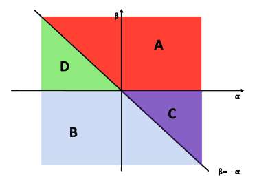
Figure 1: The quantity $-\dfrac{\beta}{\alpha}\notin(0,1)\Longleftrightarrow(\alpha,\beta)\in A\cup B.$ In $A$ we have $\beta>\min(0,-\alpha)$; in $B$ we have $\beta<\min(0,-\alpha)$. The quantity $-\dfrac{\beta}{\alpha}\in(0,1)\Longleftrightarrow(\alpha,\beta)\in C\cup D.$ In $C$ we have $\alpha>0$, $-\alpha<\beta<0$; in $D$ we have $\alpha<0$, $0<\beta<-\alpha$.

Let us describe in detail the different situations:

$(\alpha,\beta)\in A$

this means that $\beta>\min(0,-\alpha)$. If $\alpha\geq 0$ then $0<\beta\leq\alpha M_{1}(f)+\beta\leq\alpha+\beta$; if $\alpha<0$ then $0<\alpha+\beta\leq\alpha M_{1}(f)+\beta\leq\beta$. In any case we have $\alpha M_{1}(f)+\beta\geq 0$ and so $M^{\prime}_{1}(f)=(\alpha M_{1}(f)+\beta)(M_{2}(f)-M_{1}^{2}(f))\geq 0.$ As shown in Figure 2 (on the left), $M_{1}(f)$ is increasing in time and is limited on the right by the curve $\tilde{M}(t)\longrightarrow 1$ with $\tilde{M}^{\prime}(t)=(\alpha\tilde{M}+\beta)\tilde{M}(1-\tilde{M}).$

$(\alpha,\beta)\in B$

this means that $\beta<\min(0,-\alpha)$. If $\alpha\geq 0$ then $\beta\leq\alpha M_{1}(f)+\beta\leq\alpha+\beta<0$; if $\alpha<0$ then $\alpha+\beta\leq\alpha M_{1}(f)+\beta\leq\beta<0$. In any case we have $\alpha M_{1}(f)+\beta\leq 0$ and so $M^{\prime}_{1}(f)=(\alpha M_{1}(f)+\beta)(M_{2}(f)-M_{1}^{2}(f))\leq 0.$ As shown in Figure 2 (on the right), $M_{1}(f)$ is decreasing in time and is limited on the left by the curve $\tilde{M}(t)\longrightarrow 0$ with $\tilde{M}^{\prime}(t)=(\alpha\tilde{M}+\beta)\tilde{M}(1-\tilde{M}).$

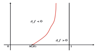
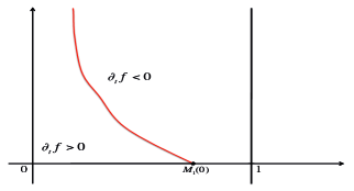
Figure 2: On the left: evolution of $M_{1}(t)$ in the case $(\alpha,\beta)\in A$. On the right: evolution of $M_{1}(t)$ in the case $(\alpha,\beta)\in B$.

Case b

$-\dfrac{\beta}{\alpha}\in(0,1)$. Figure 1 shows that it is possible if and only if $(\alpha,\beta)\in C\,\cup D$.

$(\alpha,\beta)\in C$

Figure 3 (on the left) shows two different situations:

$$M_{1}(0)>-\dfrac{\beta}{\alpha}\quad\Longrightarrow\quad M^{\prime}_{1}(f)>0;$$

$$M_{1}(0)<-\dfrac{\beta}{\alpha}\quad\Longrightarrow\quad M^{\prime}_{1}(f)<0.$$

By contrast with the previous case, the behavior changes according to the value of the first moment $M_{1}$ at initial time $t=0$. If $M_{1}(0)>-\frac{\beta}{\alpha}$ then $M_{1}(t)$ increases in time and is limited on the left by the curve $\tilde{M}(t)\longrightarrow 1$ with $\tilde{M}^{\prime}(t)=(\alpha\tilde{M}+\beta)\tilde{M}(1-\tilde{M}).$ Conversely, if $M_{1}(0)<-\frac{\beta}{\alpha}$ then $M_{1}(t)$ decreases in time and is limited on the right by the curve $\tilde{M}(t)\longrightarrow 0$ with $\tilde{M}^{\prime}(t)=(\alpha\tilde{M}+\beta)\tilde{M}(1-\tilde{M}).$

$(\alpha,\beta)\in D$

Figure 3 (on the right) shows the two situations:

$$M_{1}(0)>-\dfrac{\beta}{\alpha}\quad\Longrightarrow\quad M^{\prime}_{1}(f)<0;$$

$$M_{1}(0)<-\dfrac{\beta}{\alpha}\quad\Longrightarrow\quad M^{\prime}_{1}(f)>0.$$

Also in this case, the behavior depends on the value of $M_{1}(0)$: if $M_{1}(0)>-\frac{\beta}{\alpha}$ then $M_{1}(t)$ decreases in time away from the value $-\frac{\beta}{\alpha}$; if $M_{1}(0)<-\frac{\beta}{\alpha}$ then $M_{1}(t)$ increases in time toward the value $-\frac{\beta}{\alpha}$. In any cases, the value $-\frac{\beta}{\alpha}$ is the one that dominates in time.

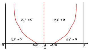
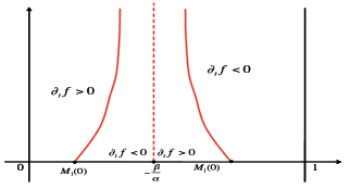
Figure 3: On the left: evolution of $M_{1}(t)$ in the case $(\alpha,\beta)\in C$. On the right: evolution of $M_{1}(t)$ in the case $(\alpha,\beta)\in D$.

From the behavior described is easy to understand what happens in the population. If we are in region $A$, there is dominance of the first of the two pure strategies that describe the game, because the dynamic encourages the state $p=1$ which corresponds to the first pure strategy. This means that in the population, those who adopt the first pure strategy survive, the others do not. In $B$ we have the opposite situation: there is the dominance of the second pure strategy and so those who adopt the first pure strategy or any other mixed strategy, do not survive. The third region $C$ is such that there is not a mixed strategy that dominates, but a priori we can not say which of the two pure strategies dominates, it all depends on the value of $M_{1}(0)$. If $M_{1}(0)>-\frac{\beta}{\alpha}$ then there is the dominance of the first pure strategy, if $M_{1}(0)<-\frac{\beta}{\alpha}$ then there is the dominance of the second pure strategy. In $D$ we have a different situation than in the previous cases: here there is coexistence between the two pure strategies and so between the two populations.

3.2 Stationary solutions

From the study of the asymptotic behavior, we expect that for $t\rightarrow\infty$ the solution of the model (27) tends to a stationary solution. We can find two classes of stationary solutions:

Type I

If we are in case b, namely $-\frac{\beta}{\alpha}\in(0,1)$, then a stationary solution is given by every density function $\overline{f}(p)$ such that

$$M_{1}(\overline{f})=-\frac{\beta}{\alpha}.$$ (34)

Type II

If we consider more general solutions, so that the probability distributions are no more absolutely continuous with respect to the Lebesgue measure, we can say that another class of stationary solutions is given by concentrated Dirac masses, i.e.:

$$f_{\overline{p}}(p)=\delta(p=\overline{p}).$$

In the following we are going to deal with these generalized solutions in a quite informal way. More rigorous arguments will be given in a future paper.

Here we want just remark that formally, since $M_{1}(f_{\overline{p}})=\overline{p}$, we have

$$f_{\overline{p}}(p)\left[(\alpha M_{1}(f_{\overline{p}})+\beta)(p-M_{1}(f_{\overline{p}}))\right]=\delta(p=\overline{p})(\alpha\overline{p}+\beta)(p-\overline{p})=0.$$

3.2.1 Linear stability of stationary solutions

This Subsection is dedicated to the study of the linear stability of stationary solutions. Denote by

$$Q(f)=f(p)\left[(\alpha M_{1}(f)+\beta)(p-M_{1}(f))\right]$$

the integral operator associated to the replicator equation. Let $\tilde{f}$ be a generalized stationary state. We linearise the operator around the state $\tilde{f}$. So for every perturbation $g$, with $\int_{0}^{1}g(p)dp=0$, we have the linear operator

$$\begin{array}[]{ll}Q^{\prime}(\tilde{f})(g)&=\lim_{h\to 0}\frac{1}{h}\left(Q(\tilde{f}+hg)-Q(\tilde{f})\right)\\ \\ &=\left[\tilde{f}M_{1}(g)+g(\alpha M_{1}(\tilde{f})+\beta)\right](p-M_{1}(\tilde{f})).\end{array}$$

Type I

we have $-1<\dfrac{\beta}{\alpha}<0$. Using (34) we obtain that the linearized equation for a perturbation $g$ is given by

$$\partial_{t}g(p)=Q^{\prime}(\overline{f})(g)=\overline{f}(p)(p-M_{1}(\overline{f}))M_{1}(g).$$ (35)

If $\int_{0}^{1}g_{0}(p)dp=0$, the same is true for $g$ for $t>0$.

Proposition 3.

Assume $-\dfrac{\beta}{\alpha}\in(0,1)$. Then, there is no continuous stationary solution $\bar{f}(p)$ to problem (27) which is linearly stable.

Proof.

To prove the result it is enough to establish the following equality

$$M_{2}(\bar{f})=(M_{1}(\bar{f}))^{2},$$ (36)

which implies that the variance of the measure $\bar{f}dp$ vanishes and so the measure has to be a Dirac mass. We take a continuous stationary solution of Type I, namely a positive function $\overline{f}$ such that its total mass is equal to 1 and $M_{1}(\overline{f})=-\frac{\beta}{\alpha}$. We perturb this state by a function $g$ of zero mass. Computing the first moment of the perturbation $g$ yields

$$M^{\prime}_{1}(g)=M_{1}(g)(M_{2}(\overline{f})-(M_{1}(\overline{f}))^{2}).$$

Setting

$$N_{1}(\bar{f}):=M_{2}(\overline{f})-(M_{1}(\overline{f}))^{2}=\int_{0}^{1}p(p+\frac{\beta}{\alpha}){\overline{f}(p)}dp,$$

we obtain:

$$M_{1}(t,g)=M_{1}(0,g)e^{tN_{1}}.$$

Moreover, setting $N_{k}(\overline{f}):=M_{k+1}(\overline{f})-M_{k}(\overline{f})M_{1}(\overline{f}),$ we have

$$M_{k}(t,g)=M_{k}(0,g)+\frac{N_{k}(\overline{f})M_{1}(0,g)}{N_{1}(\bar{f})}(e^{tN_{1}(\bar{f})}-1).$$

This means that the condition for linear stability is just:

$$N_{1}(\overline{f})=\int_{0}^{1}p(p+\frac{\beta}{\alpha})\overline{f}(p)dp\leq 0.$$

This inequality can be verified only when the equality condition is satisfied, since we already know from (32) that $N_{1}(\bar{f})\geq 0$. ∎

Type II

For the concentrated Dirac masses $f_{\overline{p}}(p)=\delta(p=\overline{p})$ we have that the linearized equation for a perturbation $g$ is given by

$$\partial_{t}g(p)=Q^{\prime}(f_{\overline{p}})(g)=g(p)(\alpha\overline{p}+\beta)(p-\overline{p}).$$ (37)

Proposition 4.

The Dirac mass solutions are linear stable if, on the support of $g(p)$, we have:

$$(\alpha\overline{p}+\beta)(p-\overline{p})\leq 0,\qquad\forall\,p\in[0,1].$$

For general perturbations, i.e.: with $supp\ g\equiv[0,1]$ we have three cases:

1. the Dirac mass concentrated in $\overline{p}=0$ is stable if $\beta<0$, which means in the original constants, $b<d$.

2. the Dirac mass concentrated in $\overline{p}=1$ is stable if $\alpha+\beta>0$, which means in the original constants, $a>c$.

3. if $-1<\frac{\beta}{\alpha}<0$, then the Dirac mass concentrated in $\overline{p}=-\frac{\beta}{\alpha}$ is stable.

4 Numerical approximation of the 1D model

We want to perform some numerical simulations with model (27). We consider some nodes

$$p_{i}\in[0,1]\qquad i=0,\dots,I,\quad(p_{0}=0,\,p_{I}=1),$$

and, using the trapezoidal rule, we obtain the following quadrature formula for the first moment $M_{1}(f)$ (for all times $t\in[0,T]$)

$$M_{1}(f)=\int_{0}^{1}pf(t,p)dp\approx\tilde{M_{1}}(f):=\displaystyle\sum_{i=0}^{I-1}\dfrac{p_{i+1}-p_{i}}{2}\,\left[p_{i+1}f(t,p_{i+1})+p_{i}f(t,p_{i})\right].$$ (38)

Clearly the above discretization is such that conservation of mass holds

$$\frac{d}{dt}\sum_{i=0}^{I-1}\dfrac{p_{i+1}-p_{i}}{2}\,\left[f(t,p_{i+1})+f(t,p_{i})\right]=$$

$$(\alpha\tilde{M_{1}}(f)+\beta)\sum_{i=0}^{I-1}\dfrac{p_{i+1}-p_{i}}{2}\left[(p_{i+1}-\tilde{M_{1}}(f))f(t,p_{i+1})+(p_{i}-\tilde{M_{1}}(f))f(t,p_{i})\right]=0,$$

provided that initially

$$\sum_{i=0}^{I-1}\dfrac{p_{i+1}-p_{i}}{2}\,\left[f_{0}(p_{i+1})+f_{0}(p_{i})\right]=1.$$

In the case of equally spaced points, $\Delta p=p_{i+1}-p_{i}$, the above property implies that

$$f(t,p_{i})\leq\frac{1}{\Delta p},\quad\forall\,t>0,\quad i=0,\ldots,I,$$

and thus the numerical solution is well-defined even when we approach a Dirac delta at the continuous level. More precisely both possible steady states are preserved by the numerical method, namely $\tilde{M_{1}}(\bar{f})=-{\beta}/{\alpha}$ and the discrete Dirac delta defined as

$$f_{\bar{p}_{i}}(p_{j})=\left\{\begin{array}[]{ll}0,&{i\neq j}\\ \displaystyle\frac{1}{\Delta p},&{i=j,\,i=1,\ldots,I-1}\\[8.5359pt] \displaystyle\frac{2}{\Delta p},&{i=j,\,i=0,I}.\end{array}\right.$$

For the time discretization we simply use a fourth order Runge-Kutta method with constant time stepping $\Delta t$ on the interval $[0,T]$. Nonnegativity of the numerical solution is achieved taking

$$\Delta t\leq|\alpha\tilde{M_{1}}(f^{n})+\beta|^{-1},$$

where $f^{n}(p_{i})=f(t^{n},p_{i})$, $t^{n}=n\Delta t$.

4.1 Numerical tests: Prisoner’s Dilemma game

One interesting example of a game is given by the so-called Prisoner’s dilemma game in which there are two players and two possible strategies. The players have two options, cooperate or defect. The payoff matrix is the following

$$C\qquad D\quad\,\,\,$$

$$\mathcal{A}=\left(\begin{array}[]{ccc}R&&S\\ T&&P\end{array}\right). \begin{array}[]{c}C\\[0.0pt] D\end{array}$$

If both players cooperate both obtain $R$ fitness units (reward payoff); if both defect, each receives $P$ (punishment payoff); if one player cooperates and the other defects, the cooperator gets $S$ (sucker’s payoff) while the defector gets $T$ (temptation payoff). The payoff values are ranked $T>R>P>S$ and $2R>T+S$. From the game theory we know that cooperators are always dominated by defectors. One of the main problems has been about the possibility of success for cooperation, which is impossible in the pure strategies models: the replicator dynamics of prisoner’s dilemma, [11], shows that cooperators are extinguished.

For the numerical tests we fix the following normalized payoff matrix:

$${\mathcal{A}}=\left(\begin{matrix}1&0\cr b&\varepsilon\end{matrix}\right),$$ (40)

with $b=1.1$ and $\varepsilon=0.001$. In this case we have $\alpha=1-b+\varepsilon<0$ and $\beta=-\varepsilon<0$ and so $\frac{\beta}{\alpha}>0$. This means that stationary solutions are expected to be given by concentrated Dirac masses (see Section 3.2). For general perturbation we have that $\bar{p}=0$ is linearly stable.

4.1.1 Test n.1

We consider the initial datum

$$f_{0}(p)=1\qquad\forall\,p\in[0,1].$$ (41)

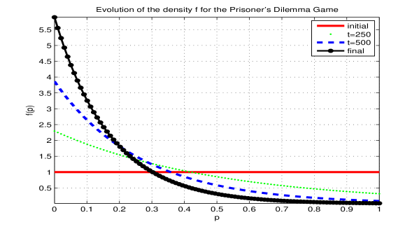
Figure 4: Prisoner’s Dilemma Game, test n.1: $b=1.1$, $\varepsilon=0.001$. Plot of the evolution over time of $f(t,p)$ for the Cauchy problem (27) with $f_{0}(p)=1$ for $T=1000$.

Figure 4 shows that the density $f$ tends to concentrate at the point $p=0$, according to what we expected.

We have studied, numerically, the $L^{\infty}$-norm of the solution $f$. Using the a priori estimate (22), we know that

$$||f||_{\infty}\leq||f_{0}(p)||_{\infty}e^{(|\alpha|+|\beta|)t}=e^{(|\alpha|+|\beta|)t},$$

and this yields

$$H(t):=Log(||f||_{\infty})\leq(|\alpha|+|\beta|)e^{Log(t)}=:E(t),\qquad\forall\,t.$$ (42)

Figure 5 shows that inequality (42) is respected.

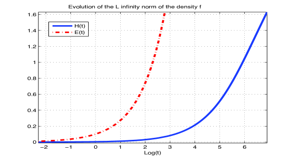
Figure 5: Prisoner’s Dilemma Game, test n.1: we have $Log(t)$ on the x-axes and $H(t)$ and $E(t)$ on the y-axes for the Cauchy problem (27) with $f_{0}(p)=1$ for $T=1000$.

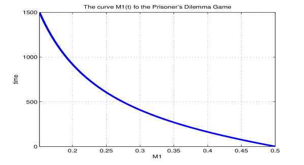
Figure 6: Prisoner’s Dilemma Game, test n.1: $b=1.1$, $\varepsilon=0.001$. Plot of the evolution of $M_{1}(t)$ vs. time $t$ for the Cauchy problem (27) with $f_{0}(p)=1$ for $T=1500$.

In the prisoner’s dilemma game we have that $(\alpha,\beta)\in B$ (see Figure 1) and we know, from game theory, that the defectors’ pure strategy dominates the cooperators’ pure strategy. The evolution in time of $M_{1}(f)$ (Figure 6) is as expected (see Figure 2 (on the right)).

We consider now a quadratic initial datum for the model (27). We have plotted the numerical results in Figure 7. As in the previous case with $f_{0}(p)=1$, we see that the density $f$ tends to concentrated at the point $p=0$ that corresponds to the defectors’ strategy.

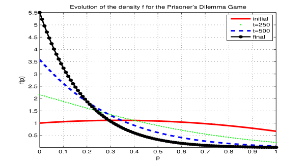
Figure 7: Prisoner’s Dilemma Game, test n.1: $b=1.1$, $\varepsilon=0.001$. Plot of the evolution over time of $f(t,p)$ for the Cauchy problem related to the model (27) with initial datum $f_{0}(p)=-p^{2}+\frac{2}{3}p+1\quad\forall\,p\in[0,1]$ for $T=1000$.

4.1.2 Test n.2

Now we want to consider an initial datum $f_{0}(p)$ with compact support in $[p_{1},p_{2}]\subset[0,1]$, with $p_{1}<p_{2}$. If we define

$$q:=\dfrac{p-p_{1}}{p_{2}-p_{1}}$$ (43)

we have that $f_{0}(q)$ has compact support in $[0,1]$. W.r.t. $q$ the average payoff (25) has the following form

$$A(q,q^{*})=\bar{\alpha}qq^{*}+\bar{\beta}q+\bar{\gamma}q^{*}+\bar{\delta},$$ (44)

with

$$\bar{\alpha}:=\alpha(p_{2}-p_{1})^{2},\quad\bar{\beta}:=\alpha(p_{2}-p_{1})p_{1}+\beta(p_{2}-p_{1}),$$ (45)

$$\bar{\gamma}:=\alpha(p_{2}-p_{1})p_{1}+\gamma(p_{2}-p_{1}),\quad\bar{\delta}:=\alpha p_{1}^{2}+(\gamma-\beta-2\delta)p_{1}+\delta.$$ (46)

The quantity

$$\dfrac{\bar{\beta}}{\bar{\alpha}}=\dfrac{1}{p_{2}-p_{1}}\left(p_{1}+\dfrac{\beta}{\alpha}\right)$$

is positive if $\frac{\beta}{\alpha}>0,$ as in the Prisoner’s Dilemma game. This means that the point $\bar{p}=p_{1}$ (corresponding to the point $\bar{q}=0$) is stable, as shown in Figure 8 that is related to the Cauchy problem (27) with the following initial datum:

$$f_{0}(p)=\begin{cases}2\qquad p\in\left[\frac{1}{4},\frac{1}{2}\right]\cup\left[\frac{3}{4},1\right]\\ 0\qquad\qquad\mbox{elsewhere.}\end{cases}$$ (47)

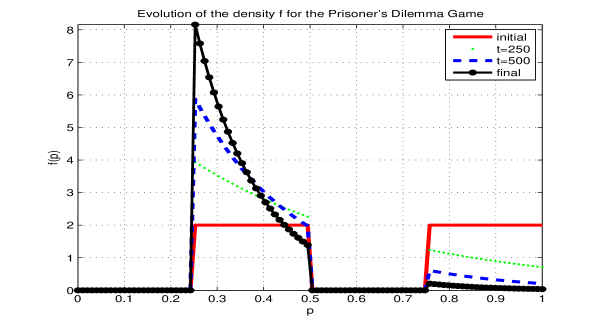
Figure 8: Prisoner’s Dilemma Game, test n.2: $b=1.1$, $\varepsilon=0.001$. Plot of the evolution over time of $f(t,p)$ for the Cauchy problem (27) with initial datum (47) for $T=1000$.

4.2 Numerical tests: Hawk or Dove Game

Another example of a game is given by the so-called Hawk or Dove game in which there are two pure strategies: hawks (H) and doves (D). While hawks escalate fights, doves retreat when the opponent escalates. The benefit of winning the fight is $b$. The cost of injury is $c$. If two hawks meet, then the expected payoff for each of them is $\frac{b-c}{2}$. The fight will escalate. One hawk wins, while the other is injured. Since both hawks are equally strong, the probability of winning or losing is $\frac{1}{2}$. If a hawk meets a dove, the hawk wins and receives payoff $b$, while the dove retreats and receives payoff $0$. If two doves meet, there will be no injury. One of them eventually wins. The expected payoff is $\frac{b}{2}$. Thus the payoff matrix is given by

$$H\qquad D\qquad$$

$$\mathcal{A}=\left(\begin{array}[]{ccc}\dfrac{b-c}{2}&&b\\ 0&&\dfrac{b}{2}\end{array}\right). \begin{array}[]{c}H\\[8.5359pt] D\end{array}$$

If $b<c$, then neither pure strategy is a Nash equilibrium. If everybody adopts the first pure strategy (H), it is best to adopt the second pure strategy (D) and vice versa. This means that hawks and doves can coexist. Selection dynamics will lead to a mixed population.

We fix $b=1$ and look for a suitable value of $c>b$ for the numerical tests. We obtain the matrix

$$\mathcal{A}=\left(\begin{array}[]{ccc}\dfrac{1-c}{2}&&1\\ 0&&\dfrac{1}{2}\end{array}\right).$$

In this case we have $-\dfrac{\beta}{\alpha}=\dfrac{1}{c}$ and $(\alpha,\beta)\in D$ if $c>1$ (see Figure 1). The function

$$f_{0}(p)=-p^{2}+\theta p+1$$ (49)

is an admissible stationary solution for the problem, namely positive, with a total mass equal to 1, and with the first momentum equal to $-\dfrac{\beta}{\alpha}$, if and only if $\theta=\frac{2}{3}$ and $c=\frac{36}{17}$. In Figure 9 we show the numerical results for the Cauchy problem (27), associated to this initial datum. We remark that the numerical scheme preserves the stationary solution.

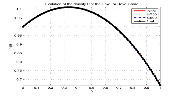
Figure 9: Hawk or Dove Game, quadratic stationary solution: we plot the evolution over time of $f(t,p)$ for the Cauchy problem (27) with initial datum (49) for $T=1000$.

As a consequence of Proposition 3, the stationary solution (49) is not linearly stable, in fact

$$M_{2}(f_{0}(p))-(M_{1}(f_{0}(p)))^{2}=\int_{0}^{1}\left(\left(-p^{3}+\dfrac{2}{3}p^{2}+p\right)\left(p-\dfrac{17}{36}\right)\right)dp\cong 0.07.$$

Actually, even small perturbations of the datum can generate large perturbations on the solutions. We consider a perturbation with zero mass for the function (49):

$$\tilde{f}_{0}(p)=-p^{2}+\dfrac{2}{3}p+1+0.02\sin(2\pi p),$$ (50)

$\forall\,p\in[0,1]$. Figure 10 shows the evolution of $f(t,p)$ for the related Cauchy problem.

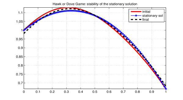
Figure 10: Hawk or Dove Game, no stability of quadratic stationary solution: we plot the evolution over time of $f(t,p)$ for the Cauchy problem (27) with initial datum (50) for $T=1000$.

The perturbed datum (50) originates the loss of the stationary solution, as seen in Figure 10. The solution of the problem evolves (slowly) towards a Dirac mass and we can see the first moment $M_{1}$ which converges to the value $-\frac{\beta}{\alpha}=0.4722$ (Figure 11), as expected since $(\alpha,\beta)$ are in the region $D$.

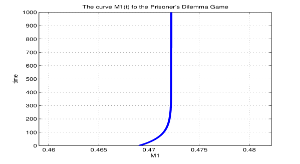
Figure 11: Hawk or Dove Game, asymptotic behavior: we have $t$ on the y-axes and $M_{1}(t)$ on the x-axes for the Cauchy problem (27) with initial datum (50) for $T=1000$.

5 Three strategies games

Assume there are three different strategies, whose interplay is ruled by the payoff matrix:

$${\mathcal{A}}=\left(\begin{matrix}a_{1}&a_{2}&a_{3}\cr a_{4}&a_{5}&a_{6}\cr a_{7}&a_{8}&a_{9}\end{matrix}\right).$$

We have a population where individuals are going to play strategy A with probability $p_{1}$, strategy B with probability $p_{2}$ and strategy C with probability $1-p_{1}-p_{2}$, for $(p_{1},p_{2})\in\mathcal{T}_{2}$, where the simplex $\mathcal{T}_{2}$ is just

$$\mathcal{T}_{2}=\{{\bf{p}}=(p_{1},p_{2})\in\mathbb{R}^{2}\,|\,p_{1},\,p_{2}\geq 0,\,p_{1}+p_{2}\leq 1\}.$$ (51)

The payoff (2) is given by

$$\begin{array}[]{ll}A({\bf{p}},{\bf{p^{*}}})=&\left(\begin{array}[]{c}p_{1}\\ p_{2}\\ 1-p_{1}-p_{2}\end{array}\right)\left(\begin{matrix}a_{1}&a_{2}&a_{3}\cr a_{4}&a_{5}&a_{6}\cr a_{7}&a_{8}&a_{9}\end{matrix}\right)\left(\begin{array}[]{c}p_{1}^{*}\\ p_{2}^{*}\\ 1-p_{1}^{*}-p_{2}^{*}\end{array}\right)\\ \\ &=(a_{1}-a_{3}-a_{7}+a_{9})p_{1}p_{1}^{*}+(a_{2}-a_{3}-a_{8}+a_{9})p_{1}p_{2}^{*}\\ \\ &+(a_{4}-a_{6}-a_{7}+a_{9})p_{1}^{*}p_{2}+(a_{5}-a_{6}-a_{8}+a_{9})p_{2}p_{2}^{*}+(a_{3}-a_{9})p_{1}\\ \\ &+(a_{7}-a_{9})p_{1}^{*}+(a_{6}-a_{9})p_{2}+(a_{8}-a_{9})p_{2}^{*}+a_{9}\\ \\ &=\alpha p_{1}p_{1}^{*}+\beta p_{1}p_{2}^{*}+\gamma p_{1}^{*}p_{2}+\delta p_{2}p_{2}^{*}+\sigma p_{1}+\eta p_{1}^{*}+\xi p_{2}+\mu p_{2}^{*}+\iota,\\ \\ \end{array}$$ (52)

with $\alpha:=a_{1}-a_{3}-a_{7}+a_{9}$, $\beta:=a_{2}-a_{3}-a_{8}+a_{9}$, $\gamma:=a_{4}-a_{6}-a_{7}+a_{9}$, $\delta:=a_{5}-a_{6}-a_{8}+a_{9}$, $\sigma:=a_{3}-a_{9}$, $\eta:=a_{7}-a_{9}$, $\xi:=a_{6}-a_{9}$, $\mu:=a_{8}-a_{9}$ and $\iota:=a_{9}$. In this case, the problem (17) is

$$\begin{cases}\partial_{t}f({\bf{p}})=F(f)\quad t\geq 0,\,{\bf{p}}\in\mathcal{T}_{2},\\ f(0,{\bf{p}})=f_{0}({\bf{p}}),\end{cases}$$ (53)

where the source term $F(f)$ is defined as follows:

$$F(f) := f({\bf{p}})[(\alpha M_{(1,0)}(f)+\beta M_{(0,1)}(f)+\sigma)(p_{1}-M_{(1,0)}(f))$$

$$+ (\gamma M_{(1,0)}(f)+\delta M_{(0,1)}(f)+\xi)(p_{2}-M_{(0,1)}(f))].$$

We consider the initial datum $f_{0}({\bf{p}})$ such that $f_{0}({\bf{p}})\geq 0$ and $\int_{\mathcal{T}_{2}}f_{0}({\bf{p}})d{\bf{p}}=1$.

Remark 2.

It is easy to prove that if

$$\dfrac{\beta\,\xi-\sigma\,\delta}{\delta\,\alpha-\gamma\,\beta}>0\qquad\mbox{and}\qquad\dfrac{\sigma\,\gamma-\xi\,\alpha}{\delta\,\alpha-\gamma\,\beta}>0,$$ (55)

then every distribution function $\bar{f}(\bf{p})$ with

$$M_{(1,0)}=\dfrac{\beta\,\xi-\sigma\,\delta}{\delta\,\alpha-\gamma\,\beta}\qquad\mbox{and}\qquad M_{(0,1)}=\dfrac{\sigma\,\gamma-\xi\,\alpha}{\delta\,\alpha-\gamma\,\beta}$$

is a stationary solution for the problem (53). Actually, by arguing as in Section 3, also Dirac masses concentrated on points are stationary solutions of these equations.

5.1 A special case: the Rock-Scissors-Paper Game

We consider the Rock-Scissors-Paper game, which is characterized by having three pure strategies such that $R_{1}$ is beaten by $R_{2}$, which is beaten by $R_{3}$, which is beaten by $R_{1}$. The outcomes of the game are tabulated as

$${\mathcal{A}}=\left(\begin{matrix}0&1&-1\cr-1&0&1\cr 1&-1&0\end{matrix}\right).$$ (56)

In the Rock-Scissors-Paper game, the constants that appear in the source term (5) have the following values: $\alpha=0$, $\beta=3$, $\sigma=-1$, $\gamma=-3$, $\delta=0$, $\xi=1$, and so

$$\dfrac{\beta\,\xi-\sigma\,\delta}{\delta\,\alpha-\gamma\,\beta}=\dfrac{\sigma\,\gamma-\xi\,\alpha}{\delta\,\alpha-\gamma\,\beta}=\dfrac{1}{3}.$$

The initial datum $f_{0}({\bf{p}})=2$ has integral over $\mathcal{T}_{2}$ equal to $1$ and the moments $M_{(1,0)}(2)=M_{(0,1)}(2)=\dfrac{1}{3}$ and so it is a stationary solution for this game. In the next Section 6 we will present the numerical results related to this stationary solution.

Now we want to present a result about the curve of changing sign for $\partial_{t}f$: for this game the source term (5) is

$$F(f)=f\,[(3M_{(0,1)}(f)-1)p_{1}+(1-3M_{(1,0)}(f))p_{2}+M_{(1,0)}(f)-M_{(0,1)}(f)],$$

and so we have that the curve $\bar{p}(t)\subset\mathbb{R}^{2}$ such that $\partial_{t}f(\bar{p}(t))=0,$ is given by

$$p_{1}(3M_{(0,1)}-1)+p_{2}(1-3M_{(1,0)})+M_{(1,0)}-M_{(0,1)}=0,\qquad\forall\,(M_{(1,0)},M_{(0,1)})\in\mathcal{T}_{2},$$ (57)

that is the straight line joining the points $(M_{(1,0)}(f),M_{(0,1)}(f))$ and $\left(\dfrac{1}{3},\dfrac{1}{3}\right)$. In the following Section 6 we will present the evolution over time of this straight line.

6 Numerical approximation for the 3-strategies model

First we want to construct a numerical method for problem (53). The domain $\mathcal{T}_{2}$ is just the triangle with vertices $(0,0)$, $(1,0)$, $(0,1)$. In order to make the numerical integrations, we fix a discretization step $\Delta p$ and a uniform triangular grid in $\mathcal{T}_{2}$ as Figure 12 shows. Each point of the grid is

$${\bf{p}}_{ij}:=(p_{1,i},p_{2,j})\qquad i=0,\dots I,\,\,j=0,\dots,I-i,$$ (58)

with $I:=\dfrac{1}{\Delta p}$. We use the notation $g_{i,j}:=g(t,p_{1,i},p_{2,j})$ for all $i=0,\dots,I$ and $j=0,\dots,I-i$ to indicate the value of a general function $g(t,p_{1},p_{2})$ at each grid point ${\bf{p}}_{ij}$.

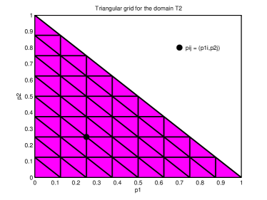
Figure 12: An example of triangular grid for the domain $\mathcal{T}_{2}$.

In order to discretize the integral of $g$ over the domain $\mathcal{T}_{2}$, we start to consider each triangle of the grid and indicate its vertices as $(x_{s},y_{s})$, for $s=1,2,3$. We define the following quantities:

$$\overline{g}:=\max(g(x_{s},y_{s}))\quad s=1,2,3$$ (59)

$$\underline{g}:=\min(g(x_{s},y_{s}))\quad s=1,2,3,$$ (60)

the maximum and the minimum value of $g$ on the triangle. On each triangle of the grid we consider a $2D$ product formula based on the trapezoidal rule:

$$\int_{\mathcal{T}_{2}} g(t,p_{1},p_{2})d{\bf{p}}=\int_{0}^{1}\,\int_{0}^{1-p_{1}}g(t,p_{1},p_{2})\,dp_{2}\,dp_{1}$$ (61)

$$\approx \dfrac{\Delta p^{2}}{2}\left[\sum_{i=0}^{I-1}\sum_{j=0}^{I-i}\left(\underline{g}_{1}+\dfrac{1}{3}(\overline{g}_{1}-\underline{g}_{1})\right)+\sum_{i=1}^{I-1}\sum_{j=0}^{I-i}\left(\underline{g}_{2}+\dfrac{1}{3}(\overline{g}_{2}-\underline{g}_{2})\right)\right],$$

where

$$\overline{g}_{1}=\max(g_{i,j},g_{i,j+1},g_{i+1,j}),\quad\underline{g}_{1}=\min(g_{i,j},g_{i,j+1},g_{i+1,j}),$$ (62)

$$\overline{g}_{2}=\max(g_{i,j},g_{i,j+1},g_{i-1,j+1}),\quad\underline{g}_{2}=\min(g_{i,j},g_{i,j+1},g_{i-1,j+1}).$$ (63)

The discretization of the first moments $M_{(1,0)}$ and $M_{(0,1)}$ is easily obtained by (61), considering the function $g(t,p_{1},p_{2})=p_{1}\,f(t,p_{1},p_{2})$ for $M_{(1,0)}(f)$ and $g(t,p_{1},p_{2})=p_{2}\,f(t,p_{1},p_{2})$ for $M_{(0,1)}(f)$.

Similarly to the one-dimensional case it can be shown that the method preserves the total mass in time, as well as discrete analogous of the steady states. As before the time discretization is done with a fourth order Runge-Kutta method with constant time stepping.

6.1 Numerical tests: The Rock-Scissors-Paper Game

We consider the Cauchy problem associated to the problem (53) for the Rock-Scissors-Paper game with the payoff matrix (56). The problem has the following equation:

$$\begin{cases}\partial_{t}f({\bf{p}})=f({\bf{p}})[(3M_{(0,1)}(f)-1)(p_{1}-M_{(1,0)}(f))\\ \quad\quad\quad\quad\quad+(1-3M_{(1,0)}(f))(p_{2}-M_{(0,1)}(f))],\\ f(0,{\bf{p}})=f_{0}({\bf{p}}).\end{cases}$$ (64)

6.1.1 Test n.1

We start with an initial datum compactly supported in $\mathcal{T}_{2}$: the sum of $s\geq 1$ truncated Gaussian functions, centered in $(p_{1}^{0,r},p_{2}^{0,r})$ for $r=1,\dots,s$. To ensure that (11) applies, we normalize the datum so that its integral over $\mathcal{T}_{2}$ is equal to $1$. Our datum is of the following type

$$f_{0}({\bf{p}}):=\dfrac{G({\bf{p}})}{\int_{\mathcal{T}_{2}}G({\bf{p}})\,d{\bf{p}}},$$ (65)

where

$$G({\bf{p}}):=\sum_{r=1}^{s}\,\max\left(\dfrac{1}{2\pi}\,e^{-K_{r}[(p_{1}-p_{1}^{0,r})^{2}+(p_{2}-p_{2}^{0,r})^{2}]}-0.01,0\right),$$ (66)

with $K_{r}>0$.

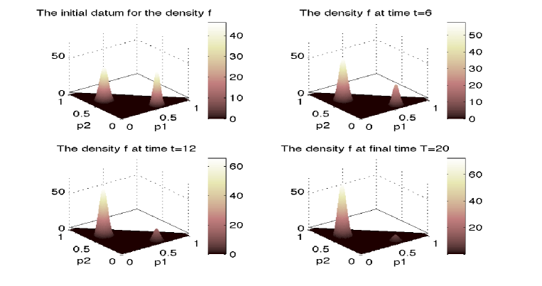
Figure 13: Rock-Scissors-Paper Game, test 1.1: the evolution of the density $f$ that is the numerical solution of the Cauchy problem (64)-(65) with $s=2$, $(p_{1}^{0,1},p_{2}^{0,1})=(\frac{1}{10},\frac{3}{5})$, $(p_{1}^{0,2},p_{2}^{0,2})=(\frac{3}{5},\frac{2}{10})$, $K_{1}=300$, $K_{2}=190$ and $T=20$.

Test 1.1

We fix $s=2$, $(p_{1}^{0,1},p_{2}^{0,1})=(\frac{1}{10},\frac{3}{5})$, $(p_{1}^{0,2},p_{2}^{0,2})=(\frac{3}{5},\frac{2}{10})$, $K_{1}=300$, $K_{2}=190$.

The graphical results (in Figure 13) shows that there is dominance of one of the groups: the initial datum is likely to have two areas of concentration, the final configuration shows only one area of concentration, and the total $L^{1}$ mass remains constantly equal to $1$ over time. The dominance group is contained in the region where $\partial_{t}f$ is positive as we can see in the Figure 14 that shows the contours of $f$ and the numerical results of the straight line $\bar{p}(t)$ of changing sign for $\partial_{t}f$ (see Subsection 5.1). We also remark that, for all $t>0$, the support of $f(t)$ is equal or a subset of the support of the initial datum $f_{0}$:

$$supp(f(t))\subseteq supp(f_{0}),\qquad\forall\,t>0.$$

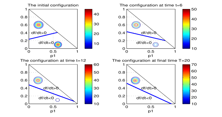
Figure 14: Rock-Scissors-Paper Game, test 1.1: the evolution over time of the contours of the density $f$ and of the curve $\bar{p}(t)$ of change of sign for $\partial_{t}\,f$ for the Cauchy problem (64)-(65) with the same data and the same parameters as the previous Figure 13.

Test 1.2

We fix $s=2$, $(p_{1}^{0,1},p_{2}^{0,1})=(\frac{1}{3},\frac{1}{3})$, $(p_{1}^{0,2},p_{2}^{0,2})=(\frac{3}{16},\frac{3}{16})$, $K_{1}=600$, $K_{2}=300$.

The graphical results (Figure 15 and Figure 16) show that the situation is different from the previous test: in this case the initial datum lies between the two regions where $\partial_{t}f$ is positive and negative and the straight line $\bar{p}(t)$ of separation between this two regions does not changes significantly over time. Therefore the configuration of the function $f$ at the final time $T$ is not very different from that at the initial time.

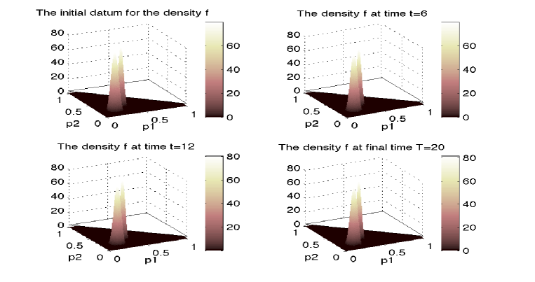
Figure 15: Rock-Scissors-Paper Game, test 1.2: the evolution of the density $f$ that is the numerical solution of the Cauchy problem (64)-(65) with $s=2$, $(p_{1}^{0,1},p_{2}^{0,1})=(\frac{1}{3},\frac{1}{3})$, $(p_{1}^{0,2},p_{2}^{0,2})=(\frac{3}{16},\frac{3}{16})$, $K_{1}=600$, $K_{2}=300$ and $T=20$.

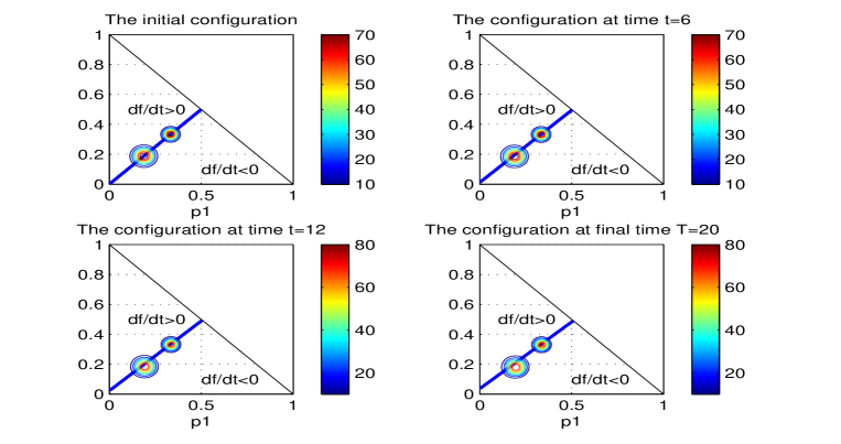
Figure 16: Rock-Scissors-Paper Game, test 1.2: the evolution over time of the contours of the density $f$ and of the curve $\bar{p}(t)$ of change of sign for $\partial_{t}\,f$ for the Cauchy problem (64)-(65) with the same data and the same parameters as the previous Figure 15.

6.1.2 Test 1.3

We fix $s=3$, $(p_{1}^{0,1},p_{2}^{0,1})=(\frac{1}{3},\frac{1}{3})$, $(p_{1}^{0,2},p_{2}^{0,2})=(\frac{3}{16},\frac{3}{16})$, $(p_{1}^{0,3},p_{2}^{0,3})=(\frac{1}{10},\frac{3}{5})$, $K_{1}=600$, $K_{2}=300$ and $K_{3}=300$.

The graphical results (Figure 17 and Figure 18) show dominance phenomena in the region where $\partial_{t}f$ is positive. Initially the three areas of concentration are located, almost entirely, in the region where $\partial_{t}f$ is negative. The time evolution shows us that, already at $t=6$, two of the three areas of concentration are in the middle between the two regions where $\partial_{t}f$ is negative and positive, then to the final time, are completely in the region where $\partial_{t}f$ is positive. So it is clear that dominance takes place in these areas.

Figure 17: Rock-Scissors-Paper Game, test 1.3: the evolution of the density $f$ that is the numerical solution of the Cauchy problem (64)-(65) with $s=3$, $(p_{1}^{0,1},p_{2}^{0,1})=(\frac{1}{3},\frac{1}{3})$, $(p_{1}^{0,2},p_{2}^{0,2})=(\frac{3}{16},\frac{3}{16})$, $(p_{1}^{0,3},p_{2}^{0,3})=(\frac{1}{10},\frac{3}{5})$, $K_{1}=600$, $K_{2}=300$, $K_{3}=300$ and $T=20$.

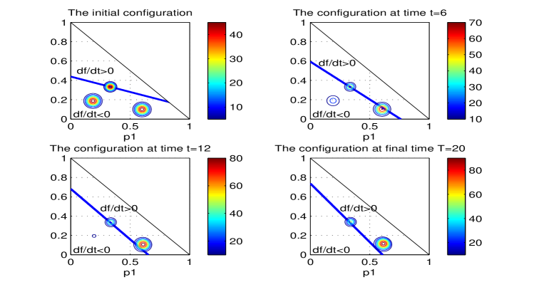
Figure 18: Rock-Scissors-Paper Game, test 1.3: the evolution over time of the contours of the density $f$ and of the curve $\bar{p}(t)$ of change of sign for $\partial_{t}\,f$ for the Cauchy problem (64)-(65) with the same data and the same parameters as the previous Figure 17.

7 Conclusions

We have considered a kinetic-like model for the evolution of a continuous mixed strategy game. The model is based on the time evolution of a density function describing the density of population adopting a given strategy. We established several analytical properties and develop some numerical discretizations useful for numerical simulations in the case of two and three strategies. Several explicit examples for two and three strategies games are reported. Of course when considering more strategies a deterministic approach may result in excessive computational requirements and stochastic simulations methods should be considered [7].

Let us finally mention that, in the situation considered so far, each player adopts a strategy and evolution over time leading to survival or not of the player. In principle it can be interesting to consider a situation in which each player can change strategy by a random mutation, so moving through the strategy space. One can introduce, to this end, a term in the equation that allows for the random change of strategy, following the ideas presented in [8]. The most natural way to model this phenomenon is to add a variation term in the equation (16), due to the probability ${\bf{p}}\in\mathcal{T}_{N-1}$

$$\partial_{t}f-D\,\triangle_{{\bf{p}}}f=f\,\left(\sum_{i=1}^{N-1}(p_{i}-M_{{\bf{e}}_{i}}(f))\left(\upsilon_{i}+\sum_{j=1}^{N-1}\vartheta_{i,j}\,M_{{\bf{e}}_{j}}(f)\right)\right),$$ (67)

with $D>0$. The new term $\triangle_{{\bf{p}}}f$ can be interpreted as a diffusion term describing the spreading of the population in the probability space from strategy to strategy, which in evolution models corresponds to a random mutation mechanism, and will be the object of a future work. A similar model has been presented recently in [14].

References

- [1] P. Abrams, Modelling the adaptive dynamics of traits involved in inter- and intraspecific interactions: an assessment of three methods, Ecol. Lett. 4, (2001) 166–175.
- [2] I. Bomze, Dynamical aspects of evolutionary stability, Mon. Math. 110, (1990) 189–206.
- [3] D. Challet, M. Marsili, Y-C. Zhang, Minority Games: Interacting Agents in Financial Markets, Oxford University Press (2005).
- [4] R.Cressman, Stability of the replicator equation with continuous strategy space, Mathematical Social Sciences 50, (2005) 127–147.
- [5] L. Desvillettes, P.-E. Jabin, S. Mischler, G. Raoul, On selection dynamics for continuous structured populations, Commun. Math. Sci. 6, (2008) 729–747.
- [6] D. Friedman, Towards evolutionary game models of financial markets, Quantitative Finance 1, (2001)
- [7] A. Galstyan, Continuous Strategy Replicator Dynamics for Multi–Agent Learning (arXiv:0904.4717v1)
- [8] S. Genieys, N. Bessonov, V. Volpert, Mathematical model of evolutionary branching Mathematical and Computer Modelling 49, (2009) 2109–2115.
- [9] J. Henriksson, T. Lundh, B. Wennberg, A model of sympatric speciation through reinforcement, Kinet. Relat. Models 3, (2010) 143–163.
- [10] J. Hofbauer, J. Oechssler, F. Riedel, Brown-von Neumann-Nash dynamics: The continuous strategy case, Games and Economic Behavior 65, (2009) 406–429.
- [11] J. Hofbauer, K. Sigmund, Evolutionary games and population dynamics, Cambridge University Press, (1998)
- [12] T.W.L. Norman, Dynamically stable sets in infinite strategy spaces, Games and Economic Behavior 62, (2008) 610–627.
- [13] J. Oechssler, F. Riedel, Evolutionary dynamics on infinite strategy spaces, Econ. Theory 17, (2001) 141–162.
- [14] M. Ruijgrok, T. W. Ruijgrok, Replicator dynamics with mutations for games with a continuous strategy space, (arXiv:nlin/0505032v2).
- [15] J.W. Weibull, Evolutionary game theory, MIT Press, Cambridge, MA (1995).