Community structure and scale-free collections of Erdős–Rényi graphs

Abstract

Community structure plays a significant role in the analysis of social networks and similar graphs, yet this structure is little understood and not well captured by most models. We formally define a community to be a subgraph that is internally highly connected and has no deeper substructure. We use tools of combinatorics to show that any such community must contain a dense Erdős–Rényi (ER) subgraph. Based on mathematical arguments, we hypothesize that any graph with a heavy-tailed degree distribution and community structure must contain a scale free collection of dense ER subgraphs. These theoretical observations corroborate well with empirical evidence. From this, we propose the Block Two-Level Erdős–Rényi (BTER) model, and demonstrate that it accurately captures the observable properties of many real-world social networks.

Introduction

Graph analysis is becoming increasingly prevalent in the quest to understand diverse phenomena like social relationships, scientific collaboration, purchasing behavior, computer network traffic, and more. We refer to graphs coming from such scenarios collectively as interaction networks. A significant amount of investigation has been done to understand the graph-theoretic properties common to interaction networks. Of particular importance is the notion of community structure. Interaction networks typically decompose into internally well-connected sets referred to as low conductance or high modularity cuts GiNe02 ; New06 . Moreover, many graphs have high clustering coefficients WaSt98 , which is indicative of underlying community structure. Communities occur in a variety of sizes, though the largest community is often much smaller than the graph itself LeLaDa08 ; LaKiSa10 . Community analysis can reveal important patterns, decomposing large collections of interactions into more meaningful components.

A Theory of Communities

One metric of the quality of a community is the modularity metric New06 . There are other measures such as conductance Ch92-book , but they are equivalent to modularity in terms of our intentions. Consider a graph $G$ (undirected) with $n$ vertices and degrees $d_{1},d_{2},\ldots,d_{n}$. Let $m=\frac{1}{2}\sum_{i=1}^{n}d_{i}$ denote the number of edges. We say a subgraph $S$ has high modularity if $S$ contains many more internal edges than predicted by a null model, which says vertices $i$ and $j$ are connected with probability $d_{i}d_{j}/2m$. (Technically, the probability is $\min(1,d_{i}d_{j}/2m)$, but we keep the notation simple for clarity.) We refer to the null model as the CL model, based on its formalization by Chung and Lu ChLu02 ; ChLu02-2 ; see also Aiello et al. AiChLu01 and the edge-configuration model of Newman et al. NeWaSt02 .

Given a high modularity subgraph $S$, we say it is a module if it does not contain any further substructures of interest; in other words, it is internally well-modeled by CL. Formally, assume $S$ has $r$ nodes with internal degrees $\hat{d}_{1},\hat{d}_{2},\ldots,\hat{d}_{r}$ and let the number of edges in $S$ be denoted by $s=\frac{1}{2}\sum_{i=1}^{r}\hat{d}_{i}$. Consider the CL model on $S$, where edge $(i,j)$ occurs with probability $\hat{d}_{i}\hat{d}_{j}/2s$. We call $S$ a module if the induced subgraph on $S$ (the subgraph internal to $S$) is modeled well by this CL model. Looking at the contrapositive, if $S$ is not a module, then $S$ itself contains a subset of vertices that should be separated out. A module can be thought of as an “atomic” substructure within a graph. In this language, we can think of community detection algorithms as breaking a graph into modules. This discussion is not complete, however, since communities are not just modules, but also internally well-connected.

Interaction networks have an abundance of triangles, a fact that Watts and Strogatz WaSt98 succinctly express through clustering coefficients. Barrat and Weigt BaWe00 defined this as

$$C=\frac{3\times\text{total number of triangles}}{\text{total number of wedges}},$$ (1)

where a wedge is a path of length 2 WaSt98 ; GiNe02 . It has been observed that $C$ “has typical values in the range of 0.1 to 0.5 in many real-world networks” GiNe02 . Moreover, our own studies have revealed that the node-level clustering coefficient (first used in WaSt98 ), $C_{i}$, defined by

$$C_{i}=\frac{\text{number of triangles incident to node }i}{\text{number of wedges centered at node }i},$$ (2)

is typically highest for small degree nodes. Large clustering coefficients are considered a manifestation of the community structures. Naturally, we expect the triangles to be largely contained within the communities due to their high internal connectivity.

We now formally define a community to be a module with a large internal clustering coefficient. More formally, we say a module is a community if the expected number of triangles is more than $(\kappa/3)\sum_{i}{\hat{d}_{i}\choose 2}$, for some constant $\kappa$. In other words, a community is tightly connected internally and has few external links. A graph has community structure if it (or at least a constant fraction of it) can be broken up into communities. The benefit of this formalism is that we can now try to understand what graphs with community structure look like.

Let us first begin by just focusing on a single community. It seems fairly intuitive that a community cannot be large while comprising only low degree vertices nor that it consists of a single high-degree node connected to degree-one vertices (a star). We can actually prove a structural theorem about a community, given our formalization. Recall that an Erdős–Rényi (ER) graph ErRe59 ; ErRe60 on $n$ vertices with connection probability $p$ is a graph such that each pair of vertices is independently connected with probability $p$. If $p$ is a constant, we call this a dense ER graph; if $p=O(1/n)$, then we call this a sparse ER graph. Using triangle bounds from extremal combinatorics and some probabilistic arguments, we can prove the following theorem.

Theorem 1.

A constant fraction of the edges in a community are contained in a dense Erdős–Rényi graph. More formally, if the community has $s$ edges, then there must be $\Omega(\sqrt{s})$ vertices with degree $\Omega(\sqrt{s})$.

This theorem is interesting because even though it is well known that ER graphs are not good models for interaction networks, they nonetheless form an important building block for the communities. We interpret this theorem as saying that the simplest possible community is just a dense ER graph. Building on this simple intuition, we think of an interaction network as consisting of a large collection of dense ER graphs.

This leads naturally to a question about the distribution of sizes of these ER components. For that, consider the power law degree distribution observed by Barabási and Albert BaAl99 and others. They show that interaction graphs exhibit heavy-tailed degree distributions such as

$$X_{d}\propto d^{-\gamma}$$ (3)

where $X_{d}$ is the number of nodes of degree $d$ and $\gamma$ is the power law exponent.

Suppose we packed nodes with a heavy-tailed degree distribution into a collection of dense ER graphs. A community of with $s$ edges would be a dense ER graph of $\sqrt{s}$ vertices of degree $\sqrt{s}$, so the size (in vertices) of the community is exactly $\sqrt{s}$. Setting $d=\sqrt{s}$, the number of such communities is proportional to

$$\frac{n/d^{\gamma}}{d}=\frac{n}{d^{\gamma+1}}.$$

This forms a scale-free distribution of communities, exactly as observed by many studies on community structure LeLaDa08 ; LaKiSa10 . Hence, we hypothesize that real-world interaction networks consist of a scale-free collection of dense Erdős–Rényi graphs. This is consistent with most of the important observed properties of these networks.

Our analysis immediately leads to connections with Dunbar’s celebrated result on “mean group sizes” of humans (reported to be around 148 with 95% confidence limits of 100–231). Empirically, this has been reported by a variety of studies HeVi09 ; LaKiSa10 ; LeLaDa08 ; GoPeVe11 . If there exists a community of size $d$, it must satisfy $n/d^{\gamma+1}\geq 1$. For the maximum community size $\bar{d}$, we have $\bar{d}\approx n^{1/(\gamma+1)}$. For $n$ being a million and $\gamma=2$, we get an estimate for a $100$, surprisingly close to Dunbar’s estimate.

As an aside, Thm. 1 also proves that CL by itself is not a good model for interaction networks. Suppose the entire graph $G$ (with $m$ edges) can be modeled as a CL graph. Since $G$ has a high clustering coefficient, then $G$ itself is a module. Hence, $G$ must have $\Omega(\sqrt{m})$ vertices with degree $\Omega(\sqrt{m})$, but this violates the tail behavior of the degree distribution.

The BTER model

Based on the idea of a graph comprising ER communities, we propose the Block Two-Level Erdős-Rényi model (BTER). The advantages of the BTER model are that it has community structure in the form of dense ER subgraphs and that it matches well with real-world graphs. We briefly describe the model here and provide a more detailed explanation and comparisons to real-world graphs in subsequent sections.

The first phase (or level) of BTER builds a collection of ER blocks in such a way that the specified degree distribution is respected. The BTER model allows one to construct a graph with any degree distribution. Real-world degree distributions might be idealized as power laws, but it is by no means a completely accurate description ClShNe09 ; SaGaRoZh11 . When the degree distribution is heavy tailed, then the BTER graph naturally has scale-free ER subgraphs. The internal connectivity of the ER graphs is specified by the user and can be tuned to match observed data.

The second phase of BTER interconnects the blocks. We assume that each node has some excess degree after the first phase. For example, if vertex $i$ should have $d_{i}$ incident edges (according to the input degree distribution), and it has $d^{\prime}_{i}$ edges from its ER block, then the excess degree is $d_{i}-d^{\prime}_{i}$. We use a CL model (which can be considered as a weighted form of ER) over the excess degrees to form the edges that connect communities.

Previous models

There are many existing models for social networks and other real-world graphs. We give a short description of some important models; for more details, we recommend the survey of Chakrabarti and Faloutsos ChFa06 . Classic examples include preferential attachment BaAl99 , small-world models WaSt98 , copying models KuRa+00 , and forest fire LeKlFa07 . Although these models may produce heavy-tailed degree distributions, their clustering coefficients of the former three models are often low SaCaWiZa10 . Even for models that give high clustering coefficients, it is difficult to predict their community structure in advance. Because of their unpredictable behavior, it is not possible to match real data with these graphs. This makes it difficult to validate against real-world interaction networks. Moreover, none of these models explain community structure, one of the most striking features of interaction graphs.

A widely used model is the Stochastic Kronecker Graph model (known as R-MAT in an early incarnation) ChZhFa04 ; LeChKlFa10 . Notably, it has been selected as the generator for the Graph 500 Supercomputer Benchmark Graph500 . Though it has some desirable properties LeChKlFa10 , it can only generate lognormal tails (after suitable addition of random noise SePiKo11 ) and does not produce high clustering coefficients SaCaWiZa10 ; PiSeKo11 . Multifractal networks are closely related to the SKG model PaLoVi10 . The random dot product model YoSc07 ; YoSc08 can be made scalable but has never been compared to real social networks. There have been successful dendogram based structures that perform community detection and link prediction in real graphs ClNeMo04 ; ClMoNe08 . The recent hyperbolic graph model BoPaKr10 ; KrPaKi+10 is based on hyperbolic geometry and has been used to performing Internet routing.

The stochastic block model BiCh09 has been used to generate better algorithms for community detection. A degree corrected version KaNe11 has been defined to deal with imprecisions in this model. A key feature of these models is that they break the graph into a constant number of relatively large blocks, and our theory shows that this model does not give a satisfactory explanation of the clustering coefficients of low degrees (which constitute a majority of the graph). The LFR community detection benchmark LaFoRa08 is also somewhat connected to this model, since it defines a set of communities and has probabilities of edges within and between these communities. We stress that these models do not attempt to match real graphs, nor do they explain the scale-free nature of communities LeLaDa08 ; LaKiSa10 . Our hypothesis and model are very different from these results, because we use a mathematical formalization to prove the existence of a scale-free dense ER collection, and the BTER model follows this theory. Nonetheless, our model can be seen as an extension of these block models, where the number and sizes of blocks form a scale-free behavior. Implicitly, our model can be seen to use a labeling scheme for vertices that depends on the degrees, and connecting vertices with probabilities depending on the labels (thereby related to the degree corrected framework of KaNe11 ).

(a) Preprocessing: Distribution of nodes into communities

(b) Phase 1: Local links within each community

(c) Phase 2: Global links across communities

Figure 1: BTER Model Construction. In the preprocessing phase, the nodes are divided into communities. In Phase 1, within-community links are generated using the ER model. In Phase 2, across-community links are generated using the CL model on the excess degrees.

Mathematical details

We provide a sketch of the proof for Thm. 1; a complete proof is provided in the supplement. Our analysis is fundamentally asymptotic, so for ease of notation we use the $O(\cdot)$, $\Omega(\cdot)$, and $\Theta(\cdot)$ to suppress constant factors. The notation $A\ll B$ indicates that there exists some absolute constant $c$ such that $A\leq cB$. We let $S$ denote the community of interest and assume that the internal degree distribution of the community $S$ is $\hat{d}_{1},\hat{d}_{2},\ldots,\hat{d}_{r}$. We denote the number of edges in $S$ by $s=\frac{1}{2}\sum_{i=1}^{r}\hat{d}_{i}$.

Based on the given distribution, let $T$ denote the expected number of triangles in $S$. Since this is a community, we demand that $T$ be at least $\kappa/3$ times the expected number of wedges, for some constant $\kappa$. This means that

$$T\geq(\kappa/3)\sum_{i}{\hat{d}_{i}\choose 2},$$ (4)

where, for convenience, we define ${d\choose 2}=0$ when $d=1$. Let $j$ be the first index such that $\hat{d}_{j}>1$. We assume that $\sum_{i>j}\hat{d}^{2}_{j}=\Omega(\sum_{i\leq r}\hat{d}^{2}_{i})$, (which effectively means there are more wedges than degree $1$ vertices). We can bound ${\hat{d}_{i}\choose 2}\geq\hat{d}^{2}_{i}/4$, and so $T=\Omega(\sum_{i}\hat{d}^{2}_{i})$. A key fact we use is the Kruskal-Katona theorem Kru63 ; Kat68 ; Fra84 which states that if a graph has $T$ triangles and $s$ edges, then $T\leq s^{3/2}$. Combining, we have

$$\sum_{i}\hat{d}^{2}_{i}\ll s^{3/2}.$$ (5)

Now, let us count the expected number of triangles based on the CL distribution. For any triple $(i,j,k)$, let $X_{ijk}$ be the indicator random variable for $(i,j,k)$ being a triangle. This occurs when all the edges $(i,j)$, $(j,k)$, and $(k,i)$ are present, and by independence, this probability is $p_{ij}p_{jk}p_{ki}$, where $p_{ij}=\hat{d}_{i}\hat{d}_{j}/2m$. The expected number of triangles $T$ can be expressed as $\hbox{\bf E}[\sum_{i<j<k}X_{ijk}]$, which (by linearity of expectation) is $\sum_{i<j<k}\hbox{\bf E}[X_{ijk}]$. Therefore,

$$T=\sum_{i<j<k}\frac{\hat{d}_{i}\hat{d}_{j}}{2s}\cdot\frac{\hat{d}_{j}\hat{d}_{k}}{2s}\cdot\frac{\hat{d}_{i}\hat{d}_{k}}{2s}\leq\frac{\left(\sum_{i}\hat{d}^{2}_{i}\right)^{3}}{8s^{3}}$$ (6)

We argued earlier that $T=\Omega(\sum_{i}\hat{d}^{2}_{i})$. We can put this bound in (6) and rearrange to get

$$s^{3/2}\ll\sum_{i}\hat{d}^{2}_{i}$$ (7)

This is the exact reverse of (5)! This means that these quantities are the same up to constant factors. When can this be satisfied? If the community consists of $\sqrt{s}$ vertices all with degree $\sqrt{s}$, then $\sum_{i}\hat{d}^{2}_{i}=\sum_{i}s=s^{3/2}$, and the conditions are exactly satisfied. Intuitively, to satisfy both (5) and (7), there have to be $\Theta(\sqrt{s})$ vertices of degree $\Theta(\sqrt{s})$. These vertices form a dense ER graph within the community proving that each community involves a constant fraction of the edges in an ER graph.

The BTER Model in Detail

The BTER model comprises an interconnected scale-free collection of communities. Intuitively, short-range connections (Phase 1) tend to be dense and lead to large clustering coefficients. Long-range connections (Phase 2) are sparse and lead to heavy-tailed degree distributions. We describe the steps in detail below.

Preprocessing

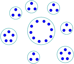
In the preprocessing step, each node of degree 2 or higher is assigned to a community. We assume the desired degree distribution $\{d_{i}\}$ is given where $d_{i}$ denotes the desired degree of node $i$. Roughly speaking, $d$ vertices of degree close to $d$ are assigned to a community (though in reality, it is somewhat involved than that because of high degree vertices.) The vertices are all partitioned into these communities, which has a scale-free behavior. Since the degree distribution is an input to the model, this step is relatively straightforward and results in a structure as shown in Fig. 1a. We let $\mathcal{G}_{k}$ denote the $k$th community and $k_{i}$ denote the community assignment for node $i$.

(a)

(b)

(c)

Figure 2: Properties of ca-AstroPh, a co-authorship network from astrophysics papers, compared with the BTER and CL models. Observe the close match of the clustering coefficients of the real data and BTER, in contrast to CL. Additionally, the eigenvalues of the BTER adjacency matrix are close to those of the real data.

(a)

(b)

(c)

Figure 3: Properties of soc-Epinions1, a social network from the Epinions website, compared with the BTER and CL models. In this case, the clustering coefficients are much smaller overall, but the BTER model is still a closer match to the real data than CL in terms of both the clustering coefficient and the eigenvalues of the adjacency matrix.

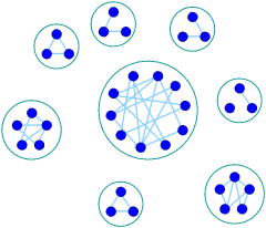
Phase 1

The local community structure is modeled as an ER graph on each community. This is illustrated in Fig. 1b. The connectivity of each community is a parameter of the model. By observing the clustering coefficient plots for real graphs, we can see that low degree vertices have a much higher clustering coefficient than higher degree ones. This suggests that small communities are much more tightly connected than larger ones, and so we adjust the connectivity accordingly. Any formula may be used; we have found empirically that the following works well in practice. We let the edge probability for community $k$ be defined as

$$\rho_{k}=\rho\left[1-\eta\left(\frac{\log(\bar{d}_{k}+1)}{\log(d_{\max}+1)}\right)^{2}\right],$$ (8)

where $\bar{d}_{k}=\min\Set{d_{i}}{i\in\mathcal{G}_{k}}$, $d_{\max}$ is the maximum degree of any node in the entire graph, and and $\rho$ and $\eta$ are parameters that can be selected for the best fit to a particular graph. (These were selected by manual experimentation for our results, but more elaborate procedures could certainly be developed.)

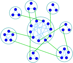
Phase 2

The global structure is determined by interconnecting the communities. We apply a CL model to the excess degree, $e_{i}$, of each node, which is computed as follows:

$$e_{i}=\begin{cases}1,&\text{if }d_{i}=1,\\ d_{i}-\rho_{k_{i}}(|\mathcal{G}_{k_{i}}|-1),&\text{otherwise},\end{cases}$$ (9)

where $|\mathcal{G}_{k}|$ is the size of community $k$. Given the $e_{i}$’s for all nodes, edges are generated by choosing two endpoints at random. Specifically, the probability of selecting node $i$ is $e_{i}/\sum_{j}e_{j}$. It is possible to produce duplicate links or self-links, but these are discarded. Phase 2 is illustrated in Fig. 1c.

Reference implementation

A MATLAB reference implementation of BTER is included in the supplementary material, including scripts to reproduce the findings in this paper. In this implementation, we have taken some care to reduce the variance in the CL model with respect to degree-one nodes. We also generate extra edges in Phase 2 to account for expected repeats and self-loops that are removed. These details are described in detail in the supplementary materials.

Results

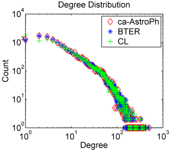
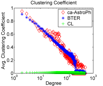
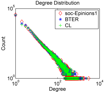
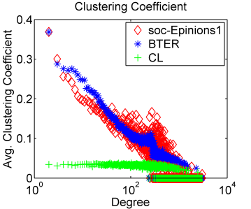
We consider comparisons of the BTER model with four real-world data sets from the SNAP collection SNAP . All the graphs are treated as undirected. Properties of these data sets are shown in Tab. 1. We compare BTER with the real data as well as the corresponding CL model. Fig. 2 shows results on a collaboration network on 124 months of data from the astrophysics (ASTRO-PH) section of the arXiv preprint server. Here, the edge probabilities in the communities are given by (8) with $\rho=0.95$ and $\eta=0.05$. Fig. 3 shows results on a who-trusts-whom online social (review) network from the Epinions website. Here, the edge probabilities in the communities are given by (8) with $\rho=0.70$ and $\eta=1.25$. Comparisons on two additional datasets listed in the table are provided in the supplement.

In the leftmost plots of Fig. 2 and Fig. 3, we see the comparison of the degree distributions. The degree distribution for ca-AstroPh has a slight “kink” mid-way and does not conform to any standard degree distribution such as lognormal or power law. Nonetheless, both BTER and CL are able to match it. The degree distribution for soc-Epinions is fairly close to a powerlaw, and matched well by both BTER and CL. In fact, these models can match any degree distribution.

The difference between BTER and CL is highlighted when we instead consider the clustering coefficient, shown in the center plots of Fig. 2 and Fig. 3. As noted previously, CL cannot have a high clustering coefficient and a heavy tail, and this is evident in these examples. BTER, on the other hand, has a close match with the observed clustering coefficients. The dense ER graphs ensure that all nodes have high clustering coefficient.

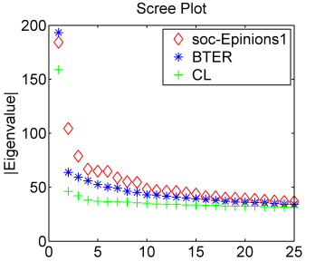
The importance of matching the clustering coefficients becomes apparent when considering other features of the graph such as the eigenvalues of the adjacency matrix, as shown in the rightmost plots of Fig. 2 and Fig. 3. For ca-AstroPh, the BTER eigenvalues are a much closer match than the CL eigenvalues because the community behavior is significant ($C=0.32$). For soc-Epinions1, the difference between the models in terms of the eigenvalues is less dramatic because the community behavior is much less evident ($C=0.07$); nonetheless, BTER is still a closer match.

Discussion

We define a community to be a subgraph that is internally well-modeled by CL (and thus has no further substructure) and highly interconnected (so that it has many triangles). We prove that any community must contain a dense ER subgraph. Therefore, any graph model that captures community structure must contain dense substructures in the form of dense ER graphs. This observation leads naturally to the BTER model, which explicitly builds communities of varying sizes and simultaneously generates a heavy tail.

Fitting the BTER model to real-world data is straightforward. The community sizes and composition in BTER are determined automatically according to the degree distribution. We currently use a simplistic procedure that assumes that all nodes in the same community have the same expected degree. Undoubtedly, this is an unrealistic assumption, but the variance of the model ensures that the degrees within a community vary considerably and Phase 2 adds connections between nodes of widely varying degrees. The connectivity of each ER block is a user-tunable parameter that can be adjusted to fit observed data. We currently prescribe a simple formula (8) and fit by trial and error, but the procedure could certainly be automated. Moreover, there is no particular requirement that $\rho_{k}$ be exactly the same for all communities with the same $\bar{d}_{k}$ (minimum degree) nor that $\rho_{k}$ be computed by a deterministic formula.

Our experimental results show that BTER has properties that are remarkably similar to real-world data sets. We contend that this makes BTER an appropriate model to use for testing algorithms and architectures designed for interaction graphs. In fact, BTER is even designed to be scalable. In particular, in Phase 2 we could compute the exact excess degree and use a matching procedure to complete the graph. The advantage of computing the excess degree in expectation is that it is more easily parallelized. In that case, the assignment to communities, the community connectivity, and the expected excess degree can all be computed in the preprocessing stage. Both Phase 1 and Phase 2 edges can be efficiently generated in parallel via a randomized procedure. Therefore, the BTER model is suitable for massive-scale modeling, such as that needed by Graph 500 Graph500 . The details of this implementation are outside the scope of the current discussion but will be considered in future work.

Our formalism captures the more advanced notion of link communities AhBaLe10 (where edges, rather than vertices, form communities). This allows vertices to participate in many communities. The notion of communities uses modules over internal degrees, so one can easily imagine a vertex in many communities. Thm. 1 is still true, and we still get a scale-free collection of ER graphs which may share vertices. We believe it is an interesting direction to extend BTER to link (and hence overlapping) communities.

Table 1: Data sets for empirical validation

	Vertices	Edges	$C$
ca-AstroPh LeKlFa07	18,772	396,100	0.32
soc-Epinions1 RiAgDo03	75,879	811,480	0.07
cit-HepPh GeGiKl03	34,546	841,754	0.15
ca-CondMat LeKlFa07	23,133	186,878	0.26

Appendix A Supporting Material

Theoretical details

The aim of this section is to prove Thm. 1, which we restate (in slightly different wording) for convenience. We set ${d\choose 2}=0$, when $d=1$. We will use small Greek letters for constants less than $1$, and small Roman letters for constants who values may exceed $1$. All constants considered are positive. We will make no attempt to optimize various constant factors in the proof. The proof is asymptotic in $s$, the number of edges of our community. That means that the proof holds for any sufficiently large $s$.

Theorem 2.

Consider a CL graph with degree sequence $\hat{d}_{1}\leq\hat{d}_{2}\leq\cdots\leq\hat{d}_{r}$ and set $s=\sum_{i}\hat{d}_{i}/2$. The quantities $c>0$ and $\kappa\in(0,1)$ are constants (independent of $s$).

Let $j$ be the smallest index such that $\hat{d}_{j}>1$, and assume that $\sum_{i>j}\hat{d}^{2}_{i}\geq cj$. Suppose the expected number of triangles generated with this degree sequence is at least $(\kappa/3)\sum_{i}{\hat{d}_{i}\choose 2}$. Then (for sufficiently large $s$), there exists a set of indices $S\subseteq\{1,\ldots,r\}$, such that $|S|=\Omega(\sqrt{s})$ and $\forall k\in S,\hat{d}_{k}=\Omega(\sqrt{s})$.

(The constants hidden in the $\Omega(\cdot)$ notation only hide a dependence on $c$ and $\kappa$.)

The proof of this theorem requires some extremal combinatorics and probability theory. We will first state some of these building blocks before describing the main proof. Henceforth, the assumptions stated in the theorem hold. An important tool is the Kruskal-Katona theorem that gives an upper bound on the number of triangles in a graph with a fixed number of edges.

Theorem 3 (Kruskal-Katona Kru63 ; Kat68 ; Fra84 ).

If a graph has $t$ triangles and $m$ edges, then $t\leq m^{3/2}$.

Since we are dealing with a graph distribution, we need some bounds on the expected number of edges.

Claim 4.

Let $E$ denote be the random variable denoting the number of edges in the CL graph defined by $\{\hat{d}_{i}\}$. Then $\hbox{\bf E}[E^{3/2}]\leq 2s^{3/2}$.

Proof.

Let $X_{ij}$ be the indicator random variable for the edge $(i,j)$ being present. Then, $E=\sum_{i<j}X_{ij}$. By construction, $\hbox{\bf E}[E]\leq s$ (we get an inequality because of possible self-loops). This is the sum of ${n\choose 2}$ independent random variables. Applying a multiplicative Chernoff bound (Theorems 4.1 and 4.3 of MoRa01 ),

$$\Pr[E\geq 2\hbox{\bf E}[E]]\leq\exp(-\hbox{\bf E}[E]/3)$$

Hence, the probability that $E\geq 2s$ is at most $\exp(-s/3)$. Let ${\cal E}$ denote the event that $E\geq 2s$. We can trivially bound $E$ by $n^{2}\leq s^{2}$. Using Bayes’ rule,

$$\hbox{\bf E}[E^{3/2}] = \Pr(\overline{{\cal E}})\hbox{\bf E}_{\overline{{\cal E}}}[E^{3/2}]+\Pr({\cal E})\hbox{\bf E}_{{\cal E}}[E^{3/2}]$$

$$\leq (2s)^{3/2}+\exp(-s/3)(s^{2})^{3/2}\leq 2s^{3/2}$$

∎

We now prove some claims about the expected number of triangles and the degree sequence.

Claim 5.

Let $T$ denote the expected number of triangles. The constants $\beta$ and $c^{\prime}$ depend only on $c$ and $\kappa$.

1. $T\geq\beta\sum_{i}\hat{d}^{2}_{i}$.

2. $\sum_{i}\hat{d}^{2}_{i}\leq c^{\prime}s^{3/2}$

Proof.

By assumptions in Thm. 2, $T\geq(\kappa/3)\sum_{i}{\hat{d}_{i}\choose 2}$. For $\hat{d}_{i}>1$, ${\hat{d}_{i}\choose 2}\geq\hat{d}^{2}_{i}/4$ (for large $\hat{d}_{i}$, it is actually much closer to $\hat{d}^{2}_{i}/2$). Hence, $T\geq(\kappa/12)\sum_{i>j}\hat{d}^{2}_{i}$, where $j$ is the smallest index of a non-degree $1$ vertex (as stated in Thm. 2). By assumption, $\sum_{i\leq j}\hat{d}^{2}_{i}=j\leq(1/c)\sum_{i>j}\hat{d}^{2}_{i}$, and $\sum_{i}\hat{d}^{2}_{i}\leq(1+1/c)\sum_{i>j}\hat{d}^{2}_{i}$. We can complete the proof of the first part with the following.

$$T\geq(\kappa/12)\sum_{i>j}\hat{d}^{2}_{i}\geq(\kappa/12)(1+1/c)^{-1}\sum_{i}\hat{d}^{2}_{i}$$

Suppose we generate a random CL graph. Let $t$ be the number of triangles and $E$ be the number of edges (both random variables). By Thm. 3, $t\leq E^{3/2}$. Taking expectations and applying Claim 4, $T\leq\hbox{\bf E}[E^{3/2}]\leq 2s^{3/2}$. Combining with the first part of this claim, $\sum_{i}\hat{d}^{2}_{i}\leq(2/\beta)s^{3/2}$. ∎

We come to the proof of the main theorem.

Proof.

(of Thm. 2) We choose $b$ to be a sufficiently large constant, and $\gamma$ to be sufficiently small. Let $\ell$ be the smallest index such that $\hat{d}_{\ell}>b\sqrt{s}$. For a triple of vertices $(i,j,k)$, let $X_{ijk}$ be the indicator random variable for $(i,j,k)$ forming a triangle. Note that $T=\hbox{\bf E}[\sum_{i<j<k}X_{ijk}]$. Then we have,

$$\hbox{\bf E}[\sum_{i<j<k}X_{ijk}]$$

$$= \sum_{i<j<k}\hbox{\bf E}[X_{ijk}]$$

$$\leq \sum_{i<j<k}\min\left(\frac{\hat{d}_{i}\hat{d}_{j}}{2s},1\right)\times\min\left(\frac{\hat{d}_{i}\hat{d}_{k}}{2s},1\right)\times\min\left(\frac{\hat{d}_{j}\hat{d}_{k}}{2s},1\right)$$

$$\leq \sum_{i<j<k}\frac{\hat{d}_{i}\hat{d}_{j}}{2s}\times\frac{\hat{d}_{i}\hat{d}_{k}}{2s}\times\min\left(\frac{\hat{d}_{j}\hat{d}_{k}}{2s},1\right)$$

$$\leq \sum_{i}\hat{d}^{2}_{i}\left[\sum_{\begin{subarray}{c}j\\ j<k\leq\ell\end{subarray}}\frac{\hat{d}^{2}_{j}\hat{d}^{2}_{k}}{8s^{3}}+\sum_{j,k\geq\ell}\frac{\hat{d}_{j}\hat{d}_{k}}{4s^{2}}\right]$$

$$\leq (\sum_{i}\hat{d}^{2}_{i})\left[\frac{(\sum_{j}\hat{d}^{2}_{j})(\sum_{k\leq\ell}\hat{d}^{2}_{k})}{8s^{3}}+\frac{(\sum_{j\geq\ell}\hat{d}_{j})^{2}}{4s^{2}}\right].$$

By the first part of Claim 5, $T\geq\beta\sum_{i}\hat{d}^{2}_{i}$. For convenience, we will replace all the independent indices above by $i$.

$$\beta\leq\frac{(\sum_{i}\hat{d}^{2}_{i})(\sum_{i\leq\ell}\hat{d}^{2}_{i})}{8s^{3}}+\frac{(\sum_{i\geq\ell}\hat{d}_{i})^{2}}{4s^{2}}$$ (10)

By Claim 5, $\sum_{i}\hat{d}^{2}_{i}\leq c^{\prime}s^{3/2}$. Furthermore, $\sum_{i}\hat{d}^{2}_{i}\geq b\sqrt{s}\sum_{i\geq\ell}\hat{d}_{i}$. Combining the two bounds, $\sum_{i\geq\ell}\hat{d}_{i}\leq(c^{\prime}/b)s$. Applying these bounds in (10) and setting constant $\tau$ appropriately,

$$\beta\leq\frac{c^{\prime}\sum_{i\leq\ell}\hat{d}^{2}_{i}}{8s^{3/2}}+(c^{\prime}/2b)^{2}$$

$$\Longrightarrow \sum_{i\leq\ell}\hat{d}^{2}_{i}\geq(8/c^{\prime})(\beta-(c^{\prime}/2b)^{2})s^{3/2}=\tau s^{3/2}$$

(By setting $b$ to be sufficiently large, we can ensure that $\tau$ is a positive constant.) Let $\ell^{\prime}$ be the smallest index such that $\hat{d}_{\ell^{\prime}}\geq\gamma\sqrt{m}$ and set $s^{\prime}=\sum_{\ell^{\prime}\leq i\leq\ell}\hat{d}_{i}$.

$$\tau s^{3/2}\leq\sum_{i\leq\ell}d^{2}_{i}\leq\gamma(s-s^{\prime})\sqrt{s}+bs^{\prime}\sqrt{s}$$

$$\Longrightarrow \tau s\leq s^{\prime}(b-\gamma)+\gamma s$$

$$\Longrightarrow s^{\prime}\geq s(\tau-\gamma)/(b-\gamma)=\Omega(s)$$

(Again, a sufficiently small $\gamma$ ensures positivity.) This means that the vertices with indices in $[\ell^{\prime},\ell]$ are totally incident to at least $\Omega(m)$ edges. All these vertices have degrees that are $\Theta(\sqrt{m})$, and hence there are $\Theta(\sqrt{m})$ such vertices. ∎

Implementation details

We give some specifics of the BTER implementation, to accompany the included MATLAB implementation.

In Phase 1, the last “community” generally has fewer than $\bar{d}_{k}$ nodes because we have run out of nodes. We have found it convenient to set $\rho_{k}=0$ for the last community since it is generally pretty small in any case.

We split the calculation of the Phase 2 edges into three subphases so that we can specially handle the degree-1 edges. The variance for degree-1 vertices in the CL model is high, so we set aside a proportion of these vertices to be handled “manually.” Let $r$ denote the number of degree-1 vertices and assumed the vertices and indexed from least degree to greatest. By default, 75% of the degree-1 vertices are handled “manually” (the exact proportion is user-definable); let $p=\lfloor 0.75r\rceil$ denote this quantity where $\lfloor\cdot\rceil$ denotes nearest integer. We update $e_{i}$ as follows:

$$e_{i}\leftarrow\begin{cases}0,&\text{for }1\leq i\leq p,\\ 1.10,&\text{for }p+1\leq i\leq r,\\ e_{i},&\text{otherwise}.\end{cases}$$

This update removes the first $p$ nodes from the CL part and also slightly raises the probability of an edge for the remaining $r-p$ degree-1 nodes. This modifications help to balance out the fact that some higher degree nodes (in expectation) which actually become degree-1 nodes in the final graph, so we need some of the degree-1 nodes (in expectation) to become higher degree in the final graph.

In Phase 2a, we set aside $q\leq p$ ($q$ even) degree-1 vertices to be connected to other degree-1 vertices. This value can be specified by the user or defaults to

$$q=2\;\left\lfloor\frac{p^{2}}{2\sum_{i}d_{i}}\right\rceil,$$

which is the expected number of degree-1-to-degree-1 edges expected in the CL model. This can be accomplished by randomly pairing the selected vertices. In all of our experiments, we use $q=0$.

In Phase 2b, we manually connect the remaining $(p-q)$ vertices to the rest of the graph. For each degree-1 vertex, we select an endpoint proportional to $e_{i}$.

In Phase 2c, we finally create the CL model. We modify the expected degrees to account for the edges used in Phase 2b and to account for duplicates. Thus, we update $e_{i}\leftarrow\eta e_{i}$ where

$$\eta=1-2\frac{p-q}{p-q+\sum_{i}e_{i}}+\beta,$$

where $\beta$ is the proportion of duplicates. We use $\beta=0.10$ in our experiments. The total number of edges generated in Phase 2c (including repeats and self-edges, which are discarded) is $\lfloor\sum_{i}e_{i}/2\rceil$.

Additional experimental results

We consider two additional experiments, as shown in Fig. 4 and Fig. 5. The graph Fig. 4 represents all the citations within a dataset on the high energy physics phenomenology section of the arXiv preprint server. For Fig. 4, we use an alternate formula for $\rho_{k}$ as follows:

$$\rho_{k}=0.7\left[1-0.6\left(\frac{\log(\bar{d}_{k}+1)}{\log(d_{\max}+1)}\right)^{3}\right].$$

And Fig. 5 shows results on a collaboration network on 124 months of data from the condensed matter (COND-MAT) section of the arXiv server. Here, the edge probabilities in the communities are given by (8) with $\rho=0.95$ and $\eta=0.95$.

(a)

(b)

(c)

Figure 4: Properties of cit-HepPh, a citation network of High Energy Physics papers, compared with the BTER and CL models.

(a)

(b)

(c)

Figure 5: Properties of ca-CondMat, a co-authorship network of Condensed Matter physics, compared with the BTER and CL models.

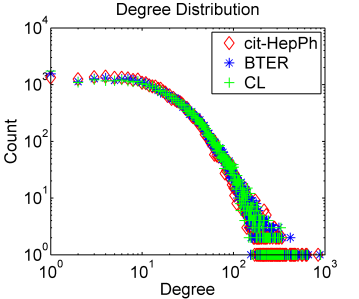
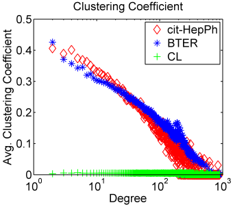
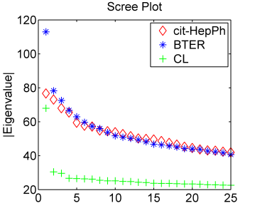
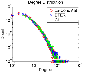
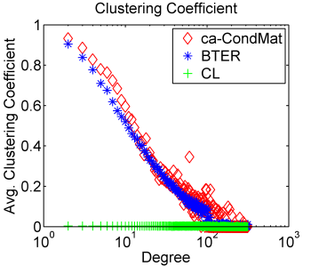
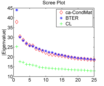
The results on these two graphs are consistent with with our earlier results. The leftmost plots show that both CL and BTER can match the degree distributions of the original graph, as expected. Again, the clustering coefficients plots in the middle highlight the strengthen of BTER, and how it differs from CL: BTER matches the clustering coefficients closely, while CL does not produce any significant number of triangles. The rightmost column shows that the eigenvalues of the adjacency matrices of BTER are closer to those of the original graph than those produced by CL.

Codes and data

The codes and data are available at http://www.sandia.gov/~tgkolda/bter_supplement/.

References and Notes

- (1) M. Girvan, M. Newman, Community structure in social and biological networks, Proceedings of the National Academy of Sciences 99, 7821 (2002).
- (2) M. E. J. Newman, Modularity and community structure in networks, Proceedings of the National Academy of Sciences 106, 21068 (2009).
- (3) D. Watts, S. Strogatz, Collective dynamics of ‘small-world’ networks, Nature 393, 440 (1998).
- (4) J. Leskovec, K. J. Lang, A. Dasgupta, M. W. Mahoney, Community structure in large networks: Natural cluster sizes and the absence of large well-defined clusters, Internet Mathematics 6, 29 (2009).
- (5) A. Lancichinetti, M. Kivelä, J. Saramäki, S. Fortunato, Characterizing the community structure of complex networks, PLoS ONE 5, e11976 (2010).
- (6) F. R. K. Chung, Spectral Graph Theory (American Mathematical Society, 1992).
- (7) F. Chung, L. Lu, The average distances in random graphs with given expected degrees, Proceedings of the National Academy of Sciences 99, 15879 (2002).
- (8) F. Chung, L. Lu, Connected components in random graphs with given degree sequences, Annals of Combinatorics 6, 125 (2002).
- (9) W. Aiello, F. Chung, L. Lu, A random graph model for power law graphs, Experimental Mathematics 10, 53 (2001).
- (10) M. Newman, D. Watts, S. Strogatz, Random graph models of social networks, Proceedings of the National Academy of Sciences 99, 2566 (2002).
- (11) A. Barrat, M. Weigt, On the properties of small-world network models, The European Physical Journal B - Condensed Matter and Complex Systems 13, 547 (2000). 10.1007/s100510050067.
- (12) P. Erdös, A. Rényi, On random graphs, Publicationes Mathematicae 6, 290 (1959).
- (13) P. Erdös, A. Rényi, On the evolution of random graphs, Publications of the Mathematical Institute of the Hungarian Academy of Sciences 5, 17 (1960).
- (14) A.-L. Barabási, R. Albert, Emergence of scaling in random networks, Science 286, 509 (1999).
- (15) A. Hernando, D. Villuendas, C. Vesperinas, M. Abad, A. Plastino, Unravelling the size distribution of social groups with information theory on complex networks (2009). ArXiv:0905.3704v3.
- (16) B. Gonçalves, N. Perra, A. Vespignani, Modeling users’ activity on twitter networks: Validation of dunbar’s number, PLoS ONE 6, e22656 (2011).
- (17) A. Clauset, C. R. Shalizi, M. E. J. Newman, Power-law distributions in empirical data, SIAM Review 51, 661 (2009).
- (18) A. Sala, H. Zheng, B. Y. Zhao, S. Gaito, G. P. Rossi, Brief announcement: revisiting the power-law degree distribution for social graph analysis, PODC ’10: Proceeding of the 29th ACM SIGACT-SIGOPS symposium on Principles of distributed computing (ACM, 2010), pp. 400–401.
- (19) D. Chakrabarti, C. Faloutsos, Graph mining: Laws, generators, and algorithms, ACM Computing Surveys 38 (2006).
- (20) R. Kumar, et al., Stochastic models for the web graph, Proceedings of the 41st Annual Symposium on Foundations of Computer Science (2000), pp. 57–65.
- (21) J. Leskovec, J. Kleinberg, C. Faloutsos, Graph evolution: Densification and shrinking diameters, ACM Transactions on Knowledge Discovery from Data 1, article no. 2 (2007).
- (22) A. Sala, et al., Measurement-calibrated graph models for social network experiments, WWW ’10 Proceedings of the 19th International Conference on the World Wide Web (ACM, New York, 2010), pp. 861–870.
- (23) D. Chakrabarti, Y. Zhan, C. Faloutsos, R-MAT: A recursive model for graph mining, SDM ’04: Proceedings of the 2004 SIAM International Conference on Data Mining (2004), pp. 442–446.
- (24) J. Leskovec, D. Chakrabarti, J. Kleinberg, C. Faloutsos, Z. Ghahramani, Kronecker graphs: An approach to modeling networks, Journal of Machine Learning Research 11, 985 (2010).
- (25) Graph 500 benchmark (2010). Available at http://www.graph500.org/Specifications.html.
- (26) C. Seshadhri, A. Pinar, T. Kolda, An in-depth study of stochastic Kronecker graphs, ICDM’11: Proceedings of the 2011 IEEE International Conference on Data Mining (2011). In press.
- (27) A. Pinar, C. Seshadhri, T. G. Kolda, The similarity between Stochastic Kronecker and Chung-Lu graph models (2011). ArXiv:1110.4925.
- (28) G. Palla, L. Lovász, T. Vicseka, Multifractal network generator, Proceedings of the National Academy of Sciences 107, 7640 (2010).
- (29) S. J. Young, E. R. Scheinerman, Random dot product graph models for social networks, WAW’07: Proceedings of the 5th International Conference on Algorithms and Models for the Web Graph, A. Bonato, F. Chung, eds. (Springer Berlin/Heidelberg, 2007), vol. 4863 of Lecture Notes in Computer Science, pp. 138–149.
- (30) S. J. Young, E. R. Scheinerman, Directed random dot product graphs, Internet Mathematics 5, 91 (2008).
- (31) A. Clauset, M. E. J. Newman, C. Moore, Finding community structure in very large networks, Physical Review E 70, 066111 (2004).
- (32) A. Clauset, C. Moore, M. E. J. Newman, Hierarchical structure and the prediction of missing links in networks, Nature 453, 98 (2008).
- (33) M. Boguna, F. Papadopoulos, D. Krioukov, Sustaining the internet with hyperbolic mapping, Nature Communications 1, 62 (2010).
- (34) D. Krioukov, F. Papadopoulos, M. Kitsak, A. Vahdat, M. Boguna, Hyperbolic geometry of complex networks, Physical Review E 82, 036106 (2010).
- (35) P. J. Bickel, A. Chen, A nonparametric view of network models and Newman-Girvan and other modularities, Proceedings of the National Academy of Sciences 103, 8577 (2006).
- (36) B. Karrer, M. E. J. Newman, Stochastic blockmodels and community structure in networks, Physical Review E 83, 21068 (2011).
- (37) A. Lancichinetti, S. Fortunato, F. Radicchi, Benchmark graphs for testing community detection algorithms, Physical Review E 78, 046110 (2008).
- (38) J. B. Kruskal, The number of simplices in a complex, Mathematical Optimization Techniques, R. Bellman, ed. (Cambridge University Press, London, 1963), pp. 251–278.
- (39) G. Katona, A theorem of finite sets, Theory of Graphs: Proceedings of the Colloquium held at Tihany, Hungary, Sept. 1966 (Academic Press and Akadémiai Kaidó, Budapest, 1968), pp. 187–207.
- (40) P. Frankl, A new short proof for the Kruskal-Katona theorem, Discrete Mathematics 48, 327 (1984).
- (41) SNAP: Stanford Network Analysis Project. Available at http://snap.stanford.edu/.
- (42) Y.-Y. Ahn, J. P. Bagrow, S. Lehmann, Link communities reveal multiscale complexity in networks, Nature 466, 761 (2010).
- (43) M. Richardson, R. Agrawal, P. Domingos, Trust management for the semantic web, ISWC 2003: Proceedings of the Second Interational Semantic Web Conference (Springer Berlin/Heidelberg, 2003), vol. 2870 of Lecture Notes in Computer Science, pp. 351–368.
- (44) J. Gehrke, P. Ginsparg, J. Kleinberg, Overview of the 2003 KDD cup, ACM SIGKDD Explorations Newsletter 5, 149 (2003).
- (45) R. Motwani, P. Raghavan, Randomized Algorithms (Cambridge University Press, 2001).