B-meson Semi-inclusive Decay to $2^{-+}$ Charmonium in NRQCD and X(3872)

Abstract

The semi-inclusive B-meson decay into spin-singlet D-wave $2^{-+}$ charmonium, $B\to\eta_{c2}+X$, is studied in non-relativistic QCD (NRQCD). Both color-singlet and color-octet contributions are calculated at next-to-leading order (NLO) in the strong coupling constant $\alpha_{s}$. The non-perturbative long-distance matrix elements are evaluated using operator evolution equations. It is found that the color-singlet ${}^{1}D_{2}$ contribution is tiny, while the color-octet channels make dominant contributions. The estimated branching ratio $B(B\to\eta_{c2}+X)$ is about $0.41\,\times 10^{-4}$ in the Naive Dimensional Regularization (NDR) scheme and $1.24\,\times 10^{-4}$ in the t’Hooft-Veltman (HV) scheme, with renormalization scale $\mu=m_{b}=4.8$ GeV. The scheme-sensitivity of these numerical results is due to cancelation between ${}^{1}S_{0}^{[8]}$ and ${}^{1}P_{1}^{[8]}$ contributions. The $\mu$-dependence curves of NLO branching ratios in both schemes are also shown, with $\mu$ varying from $\frac{m_{b}}{2}$ to $2m_{b}$ and the NRQCD factorization or renormalization scale $\mu_{\Lambda}$ taken to be $2m_{c}$. Comparison of the estimated branching ratio of $B\to\eta_{c2}+X$ with the observed branching ratio of $B\to X(3872)+K$ may lead to the conclusion that $X(3872)$ is unlikely to be the $2^{-+}$ charmonium state $\eta_{c2}$.

I introduction

One of the missing states in the charmonium family, the $\eta_{c2}({}^{1}D_{2})$, is the only missing spin-singlet low-lying D-wave charmonium state. Its mass is predicted to be within 3.80 to 3.84 GeV Eichten:2004uh ; Barnes:2005pb ; Li:2009zu , which lies between the $D\bar{D}$ and the $D^{*}\bar{D}$ thresholds. The $J^{PC}$ quantum number of $\eta_{c2}$ is $2^{-+}$, thus its decay to $D\bar{D}$ is forbidden. Therefore, this is a narrow resonance state, and its main decay modes are the electromagnetic and hadronic transitions to lower-lying S-, P-wave charmonium states and the annihilation decays to light hadrons. Previously, we calculated the inclusive light hadronic decay width of the ${}^{1}D_{2}$ state at next-to-leading order (NLO) in $\alpha_{s}$ Fan:2009cj in the framework of non-relativistic QCD (NRQCD). The results show that with the total width of $\eta_{c2}$ estimated to be about 660-810 keV, the branching ratio of the electric dipole transition $\eta_{c2}\rightarrow\gamma h_{c}$ is about $(44-54)\%$, which will be useful in searching for this missing charmonium state through $\eta_{c2}\rightarrow\gamma h_{c}$ followed by $h_{c}\rightarrow\gamma\eta_{c}$ and other processes.

The NRQCD factorization methodBodwin:1994jh was adopted in our calculation of $\eta_{c2}$ light hadronic decay. Within this framework, the inclusive decay and production of heavy quarkonium can be factorized into two parts, the short-distance coefficients and the long-distance matrix elements. A color-octet heavy quark and anti-quark pair annihilated or produced at short distances can evolve into a color-singlet heavy quarkonium at long distances via electric or magnetic transitions by emitting soft gluons, This color-octet mechanism has been used to remove the infrared (IR) divergences in P-wave Bodwin:1994jh ; Huang:1996fa ; Huang:1996sw ; Huang:1996cs ; Petrelli:1997ge ; Maltoni:1999phd and D-wave He:2008xb ; Fan:2009cj ; He:2009bf charmonium decays.

Now, we turn to the B-meson non-leptonic decays, which have played an important role in discovering new resonances, especially new charmonium and charmonium-like states in recent years. The branching fractions of B-meson inclusive decays into S-wave and P-wave charmonia, of $\mathcal{O}(10^{-3})$ to $\mathcal{O}(10^{-2})$Nakamura:2010zzi , are relatively large. Therefore, we may also expect to search for D-wave charmonia in B-meson decays, and in particular to search for the spin-singlet D-wave charmonium $\eta_{c2}$ in $B\rightarrow\eta_{c2}+X$. Like the charmonium light hadronic decay, charmonium production in B-meson semi-inclusive decay may also be factorized in NRQCD as

$$\Gamma(B\rightarrow H+X)=\sum_{n}C(b\rightarrow c\bar{c}[n]+X)\langle\mathcal{O}^{H}[n]\rangle,$$ (1)

where the sum runs over all contributing Fock states. The short-distance coefficients $C(b\rightarrow c\bar{c}[n]+X)$ can be perturbatively calculated up to any order in $\alpha_{s}$; while the long-distance matrix elements $\langle\mathcal{O}^{H}[n]\rangle$ should be determined non-perturbatively. One may refer to Beneke:1998ks ; Maltoni:1999phd for more discussions on the feasibility of Eq. (1).

S-wave and P-wave charmonium production in B-meson semi-inclusive decays have already been studied by many authors in the literature Bergstrom:1994vc ; Ko:1995iv ; Fleming:1996pt ; Soares:1997ir ; Beneke:1998ks ; Maltoni:1999phd . In Beneke:1998ks ; Maltoni:1999phd , it was found that the experimentally observed branching fractions for $J/\psi$ and $\psi^{\prime}$ could be accounted for by NLO calculations, while for $\chi_{c1}$ and $\chi_{c2}$ the branching ratios were still difficult to explain. In Yuan:1997we , the branching fractions for D-wave charmonium production in B-meson semi-inclusive decays were calculated to be of $\mathcal{O}(10^{-3})$ in NRQCD at leading order (LO), where the NRQCD velocity scaling rules were used to estimate the long-distance matrix elements. Similar results but somewhat larger branching fractions were also obtained in Ko . However, the NLO QCD corrections are found to be very important in many heavy quarkonium production processes, e.g. in $e^{+}e^{-}$ annihilationNLOee , hadroproductionNLOhad1 ; NLOhad8 , and photoproductionNLOpho . Moreover, the velocity scaling rules are too rough to give a quantitative estimate for the long-distance matrix elements. Therefore, for D-wave charmonium production in B-meson semi-inclusive decays, aside from Yuan:1997we ; Ko , a NLO calculation and a better estimate for the matrix elements are necessary.

Another important motivation for carrying out this study concerns the long-standing puzzle of the nature of $X(3872)$. Previous studies assumed that the quantum numbers of the $X(3872)$ were $J^{PC}=1^{++}$, and this was supported by a number of measurements. However, the new BABAR measurement of $X(3872)\to J/\psi\pi^{+}\pi^{-}\pi^{0}$ delAmoSanchez:2010jr favors the negative-parity assignment $2^{-+}$. Nevertheless, people still argue that the observed properties of $X(3872)$ strongly disfavor the $2^{-+}$ assignmentJia:2010jn ; Burns:2010qq ; Kalashnikova:2010hv ; Ke:2011 . Recently, Mehen:2011ds proposed that the angular distributions of decay products could be used to distinguish between the $1^{++}$ and $2^{-+}$ assignments of $X(3872)$. In this paper, we will further clarify this problem by calculating the ${}^{1}D_{2}$ charmonium production rate in B-meson semi-inclusive decay. We will compare the calculated branching ratio $B\rightarrow\eta_{c2}+X$, with the experimental measurement of $Br(B\rightarrow X(3872)K)$, and then discuss if $X(3872)$ can be the $2^{-+}$ charmonium $\eta_{c2}$.

The paper is organized as follows. In Sec. II and III, decay widths of four contributing Fock states at tree and one-loop levels are calculated both in QCD and NRQCD, and finite short-distance coefficients $C(b\rightarrow c\bar{c}[n]+X)$ for different components $c\bar{c}[n]$ are obtained respectively after matching between QCD and NRQCD. Computation methods adopted in real and virtual corrections are discussed too. The long-distance matrix elements are estimated using operator evolution equations. In Sec. IV, numerical results are given and analyzed. And finally the possibility of assigning the $\eta_{c2}$ as X(3872) is discussed.

II Leading-order (LO) contribution

We use the same description as in Maltoni:1999phd ; Beneke:1998ks . The weak decay $b\rightarrow c\bar{c}+s/d$ occurs at energy scales much lower than the W boson mass $m_{W}$. Integrating out the hard scale and making Fierz transformation, we finally arrive at the effective Hamiltonian

$$H_{eff}=\frac{G_{F}}{\sqrt{2}}\sum_{q=s,d}\left\{V_{cb}^{*}V_{cq}\left[\frac{1}{3}C_{[1]}(\mu)\mathcal{O}_{1}(\mu)+C_{[8]}(\mu)\mathcal{O}_{8}(\mu)\right]-V_{tb}^{*}V_{tq}\sum_{i=3}^{6}C_{i}(\mu)\mathcal{O}_{i}(\mu)\right\},$$ (2)

where the $c\bar{c}$ pair is either in a color singlet or a color octet configuration, denoted by $\mathcal{O}_{1}$ and $\mathcal{O}_{8}$ respectively,

$$\mathcal{O}_{1} = [\bar{c}\gamma_{\mu}(1-\gamma_{5})c][\bar{b}\gamma^{\mu}(1-\gamma_{5})q],$$

$$\mathcal{O}_{8} = [\bar{c}T^{a}\gamma_{\mu}(1-\gamma_{5})c][\bar{b}T^{a}\gamma^{\mu}(1-\gamma_{5})q].$$ (3)

$\mathcal{O}_{3-6}$ are the QCD penguin operators Buchalla:1995vs . $C_{[1]}(\mu)$ and $C_{[8]}(\mu)$ are the Wilson coefficients of $\mathcal{O}_{1}$ and $\mathcal{O}_{8}$, and related to another group of coefficients $C_{+}(\mu)$ and $C_{-}(\mu)$ through

$$C_{[1]}(\mu) = 2C_{+}(\mu)-C_{-}(\mu),$$

$$C_{[8]}(\mu) = C_{+}(\mu)+C_{-}(\mu).$$ (4)

At LO, expressions for $C_{\pm}(\mu)$ are

$$C^{LO}_{\pm}(\mu)=\left[\frac{\alpha^{LO}_{s}(m_{W})}{\alpha^{LO}_{s}(\mu)}\right]^{\gamma^{(0)}_{\pm}/(2\beta_{0})},$$ (5)

with the one-loop anomalous dimension

$$\gamma^{(0)}_{\pm}=\pm\,2\,(3\mp 1),$$ (6)

and $\alpha_{s}$

$$\alpha^{LO}_{s}(\mu)=\frac{4\pi}{\beta_{0}\ln[\mu^{2}/(\Lambda^{LO}_{QCD})^{2}]},$$ (7)

where $\beta_{0}=11-\frac{2}{3}N_{f}$. We choose $m_{W}=80.399$ GeVNakamura:2010zzi , $m_{Z}=91.1876$ GeV, $m_{b}=4.8$ GeV, $N_{f}=4$, and $\Lambda^{LO}_{QCD}=128$ MeV for four flavors to adjust $\alpha_{s}(m_{Z})$ to be 0.119 for five flavors.

Only four configurations contribute to $\eta_{c2}$ production at LO in $v$, the velocity of heavy quark or anti-quark in charmonium rest frame:

$$|\eta_{c2}\rangle=\mathcal{O}(1)|{}^{1}D_{2}^{[1]}\rangle+\mathcal{O}(v)|{}^{1}P_{1}^{[8]}g\rangle+\mathcal{O}(v^{2})|{}^{1}S_{0}^{[1,8]}gg\rangle+\cdots.$$ (8)

With the Fock state expansion Eq. (8), we have

$$\Gamma(b\rightarrow\eta_{c2}X) = \Gamma(b\rightarrow{}^{1}S_{0}^{[1]}X)+\Gamma(b\rightarrow{}^{1}S_{0}^{[8]}X)+\Gamma(b\rightarrow{}^{1}P_{1}^{[8]}X)+\Gamma(b\rightarrow{}^{1}D_{2}^{[1]}X)$$

$$= C({}^{1}S_{0}^{[1]})\langle\mathcal{O}_{1}({}^{1}S_{0})\rangle+C({}^{1}S_{0}^{[8]})\langle\mathcal{O}_{8}({}^{1}S_{0})\rangle+C({}^{1}P_{1}^{[8]})\frac{\langle\mathcal{O}_{8}({}^{1}P_{1})\rangle}{m_{c}^{2}}+C({}^{1}D_{2}^{[1]})\frac{\langle\mathcal{O}_{1}({}^{1}D_{2})\rangle}{m_{c}^{4}}.$$

$\langle\mathcal{O}_{1}({}^{1}S_{0})\rangle$, $\langle\mathcal{O}_{8}({}^{1}S_{0})\rangle$, $\langle\mathcal{O}_{8}(^{1}P_{1})\rangle$ and $\langle\mathcal{O}_{1}(^{1}D_{2})\rangle$ are the production matrix elements of four-fermion operators defined in Bodwin:1994jh ; Braaten:2002fi :

$$\mathcal{O}_{1}(^{1}S_{0}) = \chi^{\dagger}\psi\left(a_{H}^{\dagger}a_{H}\right)\psi^{\dagger}\chi,$$

$$\mathcal{O}_{8}(^{1}S_{0}) = \chi^{\dagger}T^{a}\psi\left(a_{H}^{\dagger}a_{H}\right)\psi^{\dagger}T^{a}\chi,$$

$$\mathcal{O}_{8}(^{1}P_{1}) = \chi^{\dagger}(-\frac{i}{2}\overleftrightarrow{\bm{D}})T^{a}\psi\left(a_{H}^{\dagger}a_{H}\right)\cdot\psi^{\dagger}(-\frac{i}{2}\overleftrightarrow{\bm{D}})T^{a}\chi,$$

$$\mathcal{O}_{1}(^{1}D_{2}) = \chi^{\dagger}S^{ij}\psi\left(a_{H}^{\dagger}a_{H}\right)\psi^{\dagger}S^{ij}\chi,$$ (10)

where $\overleftrightarrow{\bm{D}}=\overrightarrow{\bm{D}}-\overleftarrow{\bm{D}}$ and $S^{ij}=(-\frac{i}{2})^{2}(\overleftrightarrow{D}^{i}\overleftrightarrow{D}^{j}-\frac{1}{3}\overleftrightarrow{\bm{D}}^{2}\delta^{ij})$.

We use Wolfram Mathematica 7.0.1.0, feynarts-3.4, and FeynCalc 6.0. At tree-level, the coupling vertex structure $\bar{c}\gamma_{\mu}(1-\gamma_{5})c$ restricts possible $J^{PC}$ numbers of charmonium states. Matching amplitudes in both QCD and NRQCD at LO leads to finite short-distance coefficients

$$C({}^{1}S_{0}^{[1]}) = \Gamma_{0}C_{[1]}^{2}3(1-\eta)^{2},$$

$$C({}^{1}S_{0}^{[8]}) = \Gamma_{0}C_{[8]}^{2}\frac{9}{2}(1-\eta)^{2},$$

$$C({}^{1}P_{1}^{[8]}) = 0,$$

$$C({}^{1}D_{2}^{[1]}) = 0,$$ (11)

where

$$\Gamma_{0}=\frac{G_{F}^{2}|V_{bc}|^{2}m_{b}^{3}}{216\pi(2m_{c})},\hskip 28.45274pt\eta=\frac{4m_{c}^{2}}{m_{b}^{2}},$$ (12)

and $|V_{cs}|^{2}+|V_{cd}|^{2}\approx 1$ has been used. For the LO Feynman diagram, see Fig. [1].

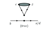
Figure 1: LO Feynman diagram of $b\rightarrow c\bar{c}+X$.

The strong dependence on renormalization scale $\mu$ of $C^{2}_{[1,8]}(\mu)$ at LO causes the results in Eq. (II) unreliable (see Fig. [2]) and calls for higher order corrections.

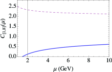
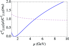
Figure 2: LO $\mu$-dependence curves of $C_{[1,8]}(\mu)$. The solid line denotes $C_{[1]}(\mu)$, and the dashed line $C_{[8]}(\mu)$. Ratios of $C_{[1,8]}^{2}(\mu)$/$C_{[1,8]}^{2}(m_{b})$ as functions of $\mu$ are also shown.

The QCD Penguin operators in Eq. (2) also contribute to non-zero tree-level decay width, although their contribution is tiny due to the smallness of $C_{3-6}(\mu)$. We will neglect their $\mu$-dependence and adopt those values given in Beneke:1998ks ; Maltoni:1999phd , for they chose the same values for $m_{b}$, $\Lambda_{QCD}^{LO}$ as ours. $C_{3}(m_{b})=0.010$, $C_{4}(m_{b})=-0.024$, $C_{5}(m_{b})=0.007$ and $C_{6}(m_{b})=-0.028$. Together with $C^{LO}_{[1]}(m_{b})=0.42$ and $C^{LO}_{[8]}(m_{b})=2.19$, the Penguin contribution is

$$\delta_{P}[{}^{1}S_{0}^{[1]}] = 2\frac{3(C_{3}-C_{5})+C_{4}-C_{6}}{C^{LO}_{[1]}}$$

$$= 0.06,$$

$$\delta_{P}[{}^{1}S_{0}^{[8]}] = 4\frac{C_{4}-C_{6}}{C^{LO}_{[8]}}$$ (13)

$$= 0.007,$$

which add corrections to tree-level short-distance coefficients in Eq. (II)

$$C({}^{1}S_{0}^{[1]}) = \Gamma_{0}C_{[1]}^{2}3(1-\eta)^{2}(1+\delta_{P}[{}^{1}S_{0}^{[1]}]),$$

$$C({}^{1}S_{0}^{[8]}) = \Gamma_{0}C_{[8]}^{2}\frac{9}{2}(1-\eta)^{2}(1+\delta_{P}[{}^{1}S_{0}^{[8]}]),$$

$$C({}^{1}P_{1}^{[8]}) = 0,$$

$$C({}^{1}D_{2}^{[1]}) = 0.$$ (14)

III NLO calculation and divergence cancellation

III.1 Real Corrections

Gluon mass regularization is adopted in our calculation, therefore $\gamma_{5}$ matrix can be treated in 4-dimension. Real correction figures are in Fig. [3].

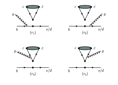
Figure 3: Real correction Feynman diagrams of $b\rightarrow c\bar{c}+X$.

Divergences are separated from the finite parts in the amplitude squared. Two kinds of divergences appear: the soft and the collinear. Three divergent regions exist: soft, soft-collinear and hard-collinear. Take ${}^{1}S_{0}^{[1]}$ for example. In the soft region, the gluon connected to the incoming bottom quark turns soft, i.e., its momentum goes to zero (($r_{1}$) of Fig. [3]); in the soft-collinear region, b-quark gluon turns soft and at the same time s/d-quark gluon is collinear with the outgoing s/d quark, or their momenta are parallel to each other (($r_{1}$) and ($r_{2}$) of Fig. [3]); and in the hard-collinear region, s/d-quark gluon runs parallel to the s/d-quark (($r_{2}$) of Fig. [3]). IR divergences in ($r_{3}$) and ($r_{4}$) of Fig. [3] cancel each other. We take the following parametrization

$$b(p_{1})\rightarrow c(p_{4})+\bar{c}(p_{3})+s/d(p_{5})+g(p_{6}),$$ (15)

and the quark propagators in four quark lines have denominators

$$N_{1} \equiv -2p_{1}\cdot p_{6}+p_{6}^{2}\,,$$

$$N_{4} \equiv 2p_{4}\cdot p_{6}+p_{6}^{2}\,,$$

$$N_{3} \equiv 2p_{3}\cdot p_{6}+p_{6}^{2}\,,$$

$$N_{5} \equiv 2p_{5}\cdot p_{6}+p_{6}^{2}\,,$$ (16)

respectively. For ${}^{1}S_{0}^{[1]}$, $p_{3}=p_{4}$ and $N_{3}=N_{4}$. Divergent terms are extracted before doing phase space integration:

soft terms $$: ~{}~{}\sim\frac{1}{N_{1}^{2}},$$

soft-collinear terms $$: ~{}~{}\sim\frac{1}{N_{1}N_{5}},$$

hard-collinear terms $$: ~{}~{}\sim\frac{1}{N_{5}},~{}\sim\frac{1}{N_{5}^{2}}.$$ (17)

Some of the hard-collinear terms are seemingly divergent but finally contribute to the finite parts. The Mandelstam variables are

$$s = (p_{1}-p_{6})^{2},$$

$$t = (p_{5}+p_{6})^{2},$$

$$u = (p_{1}-p_{5})^{2},$$ (18)

and

$$u=4m_{c}^{2}+m_{b}^{2}+\lambda^{2}-s-t,$$ (19)

with $\lambda$ the non-zero gluon mass. Rescaling all the dimensional variables with respect to $m_{b}$

$$m_{c} = \frac{m_{b}}{2}\sqrt{\eta},$$

$$\lambda = m_{b}\sqrt{\xi},$$

and

$$s = m_{b}^{2}(1-y+\xi),$$

$$t = m_{b}^{2}(1-x+\eta),$$ (21)

we finally arrive at the amplitude squared expressed using dimensionless variables $x$, $y$ instead of $s$ and $t$. Upper and lower limits of $x$ and $y$ are derived from those of $s$ and $t$ via Eq. (III.1)

$$y_{max} = 1+\xi-\frac{1}{4(1+\eta-x)}(2\eta-x+\sqrt{x^{2}-4\eta})(-2+2\xi+x-\sqrt{x^{2}-4\eta})\,,$$

$$y_{min} = 1+\xi-\frac{1}{4(1+\eta-x)}(2\eta-x-\sqrt{x^{2}-4\eta})(-2+2\xi+x+\sqrt{x^{2}-4\eta})\,,$$

$$x_{max} = 1-\xi+\eta\,,$$

$$x_{min} = 2\sqrt{\eta}\,.$$ (22)

Phase space integration over $x$ is a little bit complicated, and the Euler transformation is needed by introducing a new integration variable

$$\text{tt}\equiv\sqrt{\frac{x-2\sqrt{\eta}}{x+2\sqrt{\eta}}}$$ (23)

to replace $x$ and its integration limits

$$tt_{max} = \sqrt{\frac{\eta-2\sqrt{\eta}-\xi+1}{\eta+2\sqrt{\eta}-\xi+1}}\,,$$

$$tt_{min} = 0\,.$$ (24)

Divergences in ($r_{3}$) and ($r_{4}$) of Fig. [3] can not cancel each other for ${}^{1}S_{0}^{[8]}$, which makes divergent terms more complicated. They also produce the only IR pole, the residual divergence in ${}^{1}P_{1}^{[8]}$, which can be cancelled by absorption into the redefinitions of non-perturbative matrix elements of ${}^{1}S_{0}^{[1]}$ and ${}^{1}S_{0}^{[8]}$ states. Furthermore, there is no divergence in real correction of ${}^{1}D_{2}^{[1]}$.

III.2 Virtual Corrections

In virtual corrections, IR divergences, soft and collinear, are regulated with non-zero gluon mass like in real corrections. Ultraviolet (UV) divergences are dimensionally regulated at the amplitude level before projecting the free charm quark pair onto certain charmonium bound state of particular angular momentum and color. Virtual correction figures are in Fig. [4].

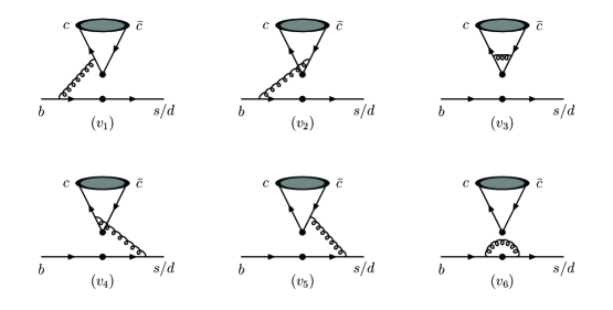
Figure 4: Virtual correction Feynman diagrams of $b\rightarrow c\bar{c}+X$.

Each diagram in Fig. [4] has an loop integration over gluon momentum $q$. For example, in $(v_{1})$ the UV divergent loop integration has the form

$$\int\frac{d^{D}q}{(2\pi)^{D}}\frac{q^{\rho}q^{\rho^{\prime}}}{(q^{2}-\lambda^{2})((p_{1}-q)^{2}-m_{b}^{2})((p_{4}-q)^{2}-m_{c}^{2})},$$ (25)

and the UV divergent term comes only from the region when $q\rightarrow\infty$

$$\int\frac{d^{D}q}{(2\pi)^{D}}\frac{q^{\rho}q^{\rho^{\prime}}}{q^{2}\cdot q^{2}\cdot q^{2}},$$ (26)

which is proportional to the D-dimensional metric tensor $g^{\rho\rho^{\prime}}$. Thus corresponding fermion chain in $(v_{1})$ reduces into

$$\Gamma_{\mu}\gamma_{\rho}\gamma_{\alpha}\otimes\gamma^{\alpha}\gamma^{\rho}\Gamma^{\mu}.$$ (27)

$\Gamma_{\mu}$ is the short form for electro-weak vertex $\gamma_{\mu}(1-\gamma_{5})$. UV divergent term extractions from structures like above are carried out upon using the Fierz transformations

$$\gamma_{\rho}\gamma_{\alpha}\Gamma_{\mu}\otimes\gamma^{\rho}\gamma^{\alpha}\Gamma^{\mu} = (16+4X\epsilon_{UV})\Gamma_{\mu}\otimes\Gamma^{\mu}+E_{X},$$

$$\Gamma_{\mu}\gamma_{\rho}\gamma_{\alpha}\otimes\gamma^{\alpha}\gamma^{\rho}\Gamma^{\mu} = (4+4Y\epsilon_{UV})\Gamma_{\mu}\otimes\Gamma^{\mu}+E_{Y},$$

$$\Gamma_{\mu}\otimes\gamma_{\rho}\gamma_{\alpha}\Gamma^{\mu}\gamma^{\alpha}\gamma^{\rho} = (4+4Z\epsilon_{UV})\Gamma_{\mu}\otimes\Gamma^{\mu}+E_{Z},$$ (28)

where the scheme dependence of $\gamma_{5}$ is fully extracted and contained in scheme-dependent variables $X$, $Y$ and $Z$,

NDR scheme $$: ~{}~{}X=-1,~{}~{}Y=Z=-2\,;$$

HV scheme $$: ~{}~{}X=-1,~{}~{}Y=Z=0\,.$$ (29)

Hence, the $\gamma_{5}$ matrix in $\Gamma_{\mu}$ can still be kept in 4-dimension when evaluating the trace formalism. Evanescent operators $E_{X}$, $E_{Y}$ and $E_{Z}$ exist only in $D\neq 4$ dimensions but vanish in $D=4$ Buchalla:1995vs . Therefore they make no contribution to the decay widths, and can be discarded throughout the calculations. Again for the ${}^{1}S_{0}^{[1]}$, self-energy diagrams of $(v_{3})$ and $(v_{6})$ can only exist for color-singlet electro-weak vertex, i.e., only $C_{[1]}(\mu)$ appears. On the contrary, the other four diagrams $(v_{1,2})$ and $(v_{4,5})$ can only have $C_{[8]}(\mu)$ electro-weak vertex. Those six diagrams only couple to the tree diagram with $C_{[1]}(\mu)$ vertex, contributing to $C^{2}_{[1]}(\mu)$ and $C_{[1]}(\mu)C_{[8]}(\mu)$ terms, respectively. IR divergence of $(v_{1})$ cancels that of $(v_{2})$, and $(v_{4})$ cancels $(v_{5})$.

Adding self-energy diagrams in Fig. [5], one can remove UV divergences in $(v_{3})$ and $(v_{6})$.

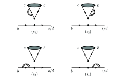
Figure 5: Self-energy correction Feynman diagrams of $b\rightarrow c\bar{c}+X$.

Explicitly,

$$(v_{3})+(s_{1})+(s_{2}) = \text{UV finite},$$

$$(v_{6})+(s_{3})+(s_{4}) = \text{UV finite},$$ (30)

where

$$(s_{1}) = -\frac{4}{3}\,i\,(4\pi\alpha_{s})N_{\epsilon}(m_{b})\left[-\frac{1}{2\epsilon_{UV}}+\frac{3}{2}\log\left(\frac{\eta}{4}\right)-\log(\xi)-2\right](tree),$$

$$(s_{2}) = -\frac{4}{3}\,i\,(4\pi\alpha_{s})N_{\epsilon}(m_{b})\left[-\frac{1}{2\epsilon_{UV}}+\frac{3}{2}\log\left(\frac{\eta}{4}\right)-\log(\xi)-2\right](tree),$$

$$(s_{3}) = -\frac{4}{3}\,i\,(4\pi\alpha_{s})N_{\epsilon}(m_{b})\left[-\frac{1}{2\epsilon_{UV}}-\log(\xi)-2\right](tree),$$

$$(s_{4}) = -\frac{4}{3}\,i\,(4\pi\alpha_{s})N_{\epsilon}(m_{b})\left[-\frac{1}{2\epsilon_{UV}}+\frac{\log(\xi)}{2}+\frac{1}{4}\right](tree),$$ (31)

with $N_{\epsilon}(m_{b})=i\,(4\pi)^{\epsilon_{UV}-2}\Gamma(\epsilon_{UV}+1)\left(\frac{\mu^{2}}{m_{b}^{2}}\right)^{\epsilon_{UV}}$. No virtual corrections to ${}^{1}P_{1}^{[8]}$ and ${}^{1}D_{2}^{[1]}$ exist accurate to NLO in $\alpha_{s}$, because of their vanishing tree-level amplitudes. This leads to a convenience directly that computation is reduced significantly. $(v_{1})+(v_{2})+(v_{4})+(v_{5})$ is still UV divergent, which needs operator renormalization, i.e., to subtract the term proportional to $\frac{1}{\epsilon_{UV}}-\gamma_{E}+\ln(4\pi)$ or equivalently make the replacement

$$\frac{1}{\epsilon_{UV}}\rightarrow\gamma_{E}-\ln(4\pi).$$ (32)

$\gamma_{E}$ is the Euler constant. To summarize our renormalization procedures. First, make mass renormalization for charm, anti-charm and bottom quarks $m_{R}\rightarrow m_{0}=m_{R}+m_{ct}$ (No such operation is needed for strange or down quarks which are taken to be massless in this paper.),

$$m_{ct}=\frac{4}{3}\,i\,(4\pi\alpha_{s})N_{\epsilon}(m_{b})\left[\frac{3}{\epsilon_{UV}}+4\right]m_{R}\,;$$ (33)

second, add the self-energy diagrams of external quark lines; finally, do operator renormalization explained above.

III.3 Residual Divergence Cancellation

We then demonstrate how the residual IR divergence is cancelled. At NLO in $\alpha_{s}$, on the QCD side,

$$\Gamma(b\rightarrow\eta_{c2}X) = C({}^{1}S_{0}^{[1]})^{QCD}_{finite+Coulomb}\langle\mathcal{O}_{1}({}^{1}S_{0})\rangle_{Born}+C({}^{1}S_{0}^{[8]})^{QCD}_{finite+Coulomb}\langle\mathcal{O}_{8}({}^{1}S_{0})\rangle_{Born}$$ (34)

$$+ C({}^{1}P_{1}^{[8]})^{QCD}_{soft}\frac{\langle\mathcal{O}_{8}({}^{1}P_{1})\rangle_{Born}}{m_{c}^{2}}+C({}^{1}D_{2}^{[1]})^{QCD}_{finite}\frac{\langle\mathcal{O}_{1}({}^{1}D_{2})\rangle_{Born}}{m_{c}^{4}},$$

while on the NRQCD side,

$$\Gamma(b\rightarrow\eta_{c2}X) = C({}^{1}S_{0}^{[1]})^{NR}\langle\mathcal{O}_{1}({}^{1}S_{0})\rangle^{NR}+C({}^{1}S_{0}^{[8]})^{NR}\langle\mathcal{O}_{8}({}^{1}S_{0})\rangle^{NR}$$

$$+ C({}^{1}P_{1}^{[8]})^{NR}\frac{\langle\mathcal{O}_{8}({}^{1}P_{1})\rangle^{NR}}{m_{c}^{2}}+C({}^{1}D_{2}^{[1]})^{NR}\frac{\langle\mathcal{O}_{1}({}^{1}D_{2})\rangle^{NR}}{m_{c}^{4}}.$$

The subscript $Coulomb$ or $soft$ means having Coulomb or soft pole. NRQCD operator mixing of ${}^{1}S_{0}^{[1,8]}$ and ${}^{1}P_{1}^{[8]}$ is shown in Fig. [6]. Similar for ${}^{1}P_{1}^{[8]}$ mixing with ${}^{1}D_{2}^{[1]}$.

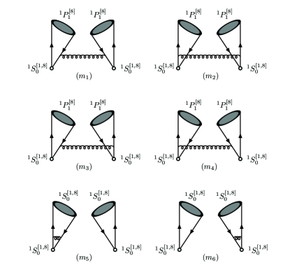
Figure 6: NRQCD operator mixing of ${}^{1}S_{0}^{[1,8]}$ and ${}^{1}P_{1}^{[8]}$.

And the non-perturbative matrix elements up to NLO in $\alpha_{s}$ are

$$\langle\mathcal{O}_{1}({}^{1}S_{0})\rangle^{NR} = \langle\mathcal{O}_{1}({}^{1}S_{0})\rangle_{Born}+\langle\mathcal{O}_{1}({}^{1}S_{0})\rangle_{Coulomb}-\frac{\alpha_{s}}{4\pi}(\ln\frac{\lambda^{2}}{\mu_{\Lambda}^{2}}+\frac{1}{3})(\frac{16}{3})\frac{\langle\mathcal{O}_{8}({}^{1}P_{1})\rangle_{Born}}{m_{c}^{2}},$$

$$\langle\mathcal{O}_{8}({}^{1}S_{0})\rangle^{NR} = \langle\mathcal{O}_{8}({}^{1}S_{0})\rangle_{Born}+\langle\mathcal{O}_{8}({}^{1}S_{0})\rangle_{Coulomb}$$

$$- \frac{\alpha_{s}}{4\pi}(\ln\frac{\lambda^{2}}{\mu_{\Lambda}^{2}}+\frac{1}{3})(\frac{16}{3})\left(C_{F}\frac{\langle\mathcal{O}_{1}({}^{1}P_{1})\rangle_{Born}}{2N_{c}m_{c}^{2}}+B_{F}\frac{\langle\mathcal{O}_{8}({}^{1}P_{1})\rangle_{Born}}{m_{c}^{2}}\right),$$

$$\langle\mathcal{O}_{8}({}^{1}P_{1})\rangle^{NR} = \langle\mathcal{O}_{8}({}^{1}P_{1})\rangle_{Born}+\langle\mathcal{O}_{8}({}^{1}P_{1})\rangle_{Coulomb}$$ (35)

$$- \frac{\alpha_{s}}{4\pi}(\ln\frac{\lambda^{2}}{\mu_{\Lambda}^{2}}+\frac{1}{3})(\frac{16}{3})\left(C_{F}\frac{\langle\mathcal{O}_{1}({}^{1}D_{2})\rangle_{Born}}{2N_{c}m_{c}^{2}}+B_{F}\frac{\langle\mathcal{O}_{8}({}^{1}D_{2})\rangle_{Born}}{m_{c}^{2}}\right).$$

$B_{F}=\frac{5}{12}$. The Coulomb singularity in $(m_{5})$ and $(m_{6})$ of Fig. [6] is extracted and related to the tree-level matrix element in the following way

$$\langle\mathcal{O}_{[n]}(c\bar{c})\rangle_{Coulomb}=\mathcal{C}_{[n]}\frac{\pi\alpha_{s}}{2v}\langle\mathcal{O}_{[n]}(c\bar{c})\rangle_{Born},$$ (36)

with the color factor

$$\mathcal{C}_{[n]}=\begin{cases}C_{F}=\frac{4}{3},&\text{n=1\,\,\, color-singlet $c\bar{c}$}\,;\\ -\frac{1}{2N_{c}}=-\frac{1}{6},&\text{n=8\,\,\, color-octet $c\bar{c}$}\,,\end{cases}$$ (37)

leading to

$$\Gamma(b\rightarrow\eta_{c2}X) = C({}^{1}S_{0}^{[1]})^{NR}\langle\mathcal{O}_{1}({}^{1}S_{0})\rangle_{Born}+C({}^{1}S_{0}^{[1]})_{Born}\langle\mathcal{O}_{1}({}^{1}S_{0})\rangle_{Coulomb}$$ (38)

$$- C({}^{1}S_{0}^{[1]})_{Born}\frac{\alpha_{s}}{4\pi}(\ln\frac{\lambda^{2}}{\mu_{\Lambda}^{2}}+\frac{1}{3})(\frac{16}{3})\frac{\langle\mathcal{O}_{8}({}^{1}P_{1})\rangle_{Born}}{m_{c}^{2}}$$

$$+ C({}^{1}S_{0}^{[8]})^{NR}\langle\mathcal{O}_{8}({}^{1}S_{0})\rangle_{Born}+C({}^{1}S_{0}^{[8]})_{Born}\langle\mathcal{O}_{8}({}^{1}S_{0})\rangle_{Coulomb}$$

$$- C({}^{1}S_{0}^{[8]})_{Born}\frac{\alpha_{s}}{4\pi}(\ln\frac{\lambda^{2}}{\mu_{\Lambda}^{2}}+\frac{1}{3})(\frac{16}{3})B_{F}\frac{\langle\mathcal{O}_{8}({}^{1}P_{1})\rangle_{Born}}{m_{c}^{2}}$$

$$+ C({}^{1}P_{1}^{[8]})^{NR}\frac{\langle\mathcal{O}_{8}({}^{1}P_{1})\rangle_{Born}}{m_{c}^{2}}+C({}^{1}D_{2}^{[1]})^{NR}\frac{\langle\mathcal{O}_{1}({}^{1}D_{2})\rangle_{Born}}{m_{c}^{4}}.$$

Matching Eq. (34) and Eq. (38), one can get the finite short-distance coefficients accurate to one-loop level

$$C({}^{1}S_{0}^{[1]})^{NR} = C({}^{1}S_{0}^{[1]})^{QCD}_{finite}\,,$$

$$C({}^{1}S_{0}^{[8]})^{NR} = C({}^{1}S_{0}^{[8]})^{QCD}_{finite}\,,$$

$$C({}^{1}P_{1}^{[8]})^{NR} = C({}^{1}P_{1}^{[8]})^{QCD}_{soft}$$

$$+ C({}^{1}S_{0}^{[1]})_{Born}\frac{\alpha_{s}}{4\pi}(\ln\frac{\lambda^{2}}{\mu_{\Lambda}^{2}}+\frac{1}{3})(\frac{16}{3})$$

$$+ C({}^{1}S_{0}^{[8]})_{Born}\frac{\alpha_{s}}{4\pi}(\ln\frac{\lambda^{2}}{\mu_{\Lambda}^{2}}+\frac{1}{3})(\frac{16}{3})B_{F}\,,$$

$$C({}^{1}D_{2}^{[1]})^{NR} = C({}^{1}D_{2}^{[1]})^{QCD}_{finite}\,.$$ (39)

Coulomb singularities in $C({}^{1}S_{0}^{[1]})^{QCD}$ and $C({}^{1}S_{0}^{[8]})^{QCD}$ and soft divergence in $C({}^{1}P_{1}^{[8]})^{QCD}$ are absorbed into the long-distance matrix elements $\langle\mathcal{O}_{1}({}^{1}S_{0})\rangle^{NR}$ and $\langle\mathcal{O}_{8}({}^{1}S_{0})\rangle^{NR}$. There is no residual soft divergence in real correction to ${}^{1}D_{2}^{[1]}$ because of the absence of tree-level amplitude of ${}^{1}P_{1}^{[8]}$. Considering its vanishing virtual correction, the NLO correction to ${}^{1}D_{2}^{[1]}$ is finite. One-loop level short-distance coefficient can be expressed in the common form

$$C(b\rightarrow c\bar{c}[n]+x)=\Gamma_{0}\frac{\alpha_{s}}{4\pi}(C^{2}_{[1]}g_{1}[n]+2C_{[1]}C_{[8]}g_{2}[n]+C^{2}_{[8]}g_{3}[n]),$$ (40)

and $g_{1}[n]$, $g_{2}[n]$ and $g_{3}[n]$ of ${}^{1}S_{0}^{[1]}$, ${}^{1}S_{0}^{[8]}$ and ${}^{1}P_{1}^{[8]}$ were calculated in Beneke:1998ks ; Maltoni:1999phd . We list them in Appendix. B. For ${}^{1}D_{2}^{[1]}$, our results are new:

$$g_{1}[{}^{1}D_{2}^{[1]}] = 0,$$

$$g_{2}[{}^{1}D_{2}^{[1]}] = 0,$$

$$g_{3}[{}^{1}D_{2}^{[1]}] = \frac{8}{135}\left(2\eta^{3}-9\eta^{2}+18\eta-6\log(\eta)-11\right).$$ (41)

III.4 Evaluation of long-distance matrix elements

Due to lack of experimental information on the matrix elements of D-wave operators, we can not extract them from experiments and have to invoke some theoretical estimates. The color-singlet matrix element $\langle\mathcal{O}_{1}({}^{1}D_{2})\rangle$ may be determined by potential models with input parameters, while the color-octet matrix elements may be estimated using the operator evolution equations. Matrix elements $\langle\mathcal{O}_{8}({}^{1}P_{1})\rangle^{NR}$, $\langle\mathcal{O}_{1}({}^{1}S_{0})\rangle^{NR}$ and $\langle\mathcal{O}_{8}({}^{1}S_{0})\rangle^{NR}$ are renormalized in NRQCD, and thus have $\mu_{\Lambda}$-dependence, and this can be explicitly shown by deriving the quantities on both sides of Eq. (III.3) with respect to $\mu_{\Lambda}$:

$$\frac{d\langle\mathcal{O}_{1}({}^{1}S_{0})\rangle^{NR}}{d\ln\mu_{\Lambda}} = \frac{\alpha_{s}}{4\pi}\frac{32}{3}\frac{\langle\mathcal{O}_{8}({}^{1}P_{1})\rangle_{Born}}{m_{c}^{2}},$$

$$\frac{d\langle\mathcal{O}_{8}({}^{1}S_{0})\rangle^{NR}}{d\ln\mu_{\Lambda}} = \frac{\alpha_{s}}{4\pi}\frac{32}{3}B_{F}\frac{\langle\mathcal{O}_{8}({}^{1}P_{1})\rangle_{Born}}{m_{c}^{2}},$$

$$\frac{d\langle\mathcal{O}_{8}({}^{1}P_{1})\rangle^{NR}}{d\ln\mu_{\Lambda}} = \frac{\alpha_{s}}{4\pi}\frac{32}{3}C_{F}\frac{\langle\mathcal{O}_{1}({}^{1}D_{2})\rangle_{Born}}{2N_{c}m_{c}^{2}}.$$ (42)

Eq. (III.4) has the same form as Eq. (45) in Fan:2009cj , where the IR divergence is regularized in dimensional regularization scheme. This is because the operator evolution equations have nothing to do with the IR divergent parts. The solutions are

$$\langle\mathcal{O}_{8}({}^{1}P_{1})(\mu_{\Lambda})\rangle^{NR} = \frac{1}{2N_{c}}\frac{8C_{F}}{3m_{c}^{2}b_{0}}\ln\frac{\alpha_{s}(\mu_{\Lambda_{0}})}{\alpha_{s}(\mu_{\Lambda})}\langle\mathcal{O}_{1}({}^{1}D_{2})\rangle_{Born},$$

$$\langle\mathcal{O}_{1}({}^{1}S_{0})(\mu_{\Lambda})\rangle^{NR} = \frac{1}{2N_{c}}\frac{C_{F}}{2}\Big{(}\frac{8}{3m_{c}^{2}b_{0}}\ln\frac{\alpha_{s}(\mu_{\Lambda_{0}})}{\alpha_{s}(\mu_{\Lambda})}\Big{)}^{2}\langle\mathcal{O}_{1}({}^{1}D_{2})\rangle_{Born},$$

$$\langle\mathcal{O}_{8}({}^{1}S_{0})(\mu_{\Lambda})\rangle^{NR} = \frac{1}{2N_{c}}\frac{C_{F}B_{F}}{2}\Big{(}\frac{8}{3m_{c}^{2}b_{0}}\ln\frac{\alpha_{s}(\mu_{\Lambda_{0}})}{\alpha_{s}(\mu_{\Lambda})}\Big{)}^{2}\langle\mathcal{O}_{1}({}^{1}D_{2})\rangle_{Born},$$ (43)

where we take $m_{c}=1.5$ GeV, $b_{0}=\frac{11C_{A}}{6}-\frac{N_{f}}{3}$, $C_{A}=3$, $N_{f}$=3, $\Lambda^{LO}_{QCD}=153$ MeV for LO, and $\Lambda_{QCD}=399$ MeV for NLO.

The initial matrix elements like $\langle\mathcal{O}_{8}({}^{1}P_{1})(\mu_{\Lambda_{0}})\rangle$ at starting scale $\mu_{\Lambda_{0}}=m_{c}v$, where $v^{2}=0.25$, are eliminated. One could refer to Fan:2009cj for reasonability of doing so. The evolution equation method for determining the long-distance matrix elements has been used in estimating the D-wave charmonium state light hadronic decay width and $h_{c}$ decay widthFan:2009cj ; He:2009bf ; He:2008xb ; Fan:2010huyu . For $h_{c}$, the evolution equation could give a prediction for light hadronic decay width within about 30% error when compared to experimental extractionFan:2010huyu . That means the operator evolution equation is a good method to evaluate the P-wave long-distance matrix element, and can be extended to D-wave case, which is lack of experimental data.

IV results and discussions

The long-distance CS D-wave matrix element is related to the second derivative of the radial wave function at the origin

$$\langle\mathcal{O}_{1}(n{}^{1}D_{2})\rangle=(2J+1)\langle n{}^{1}D_{2}|\mathcal{O}_{1}(n{}^{1}D_{2})|n{}^{1}D_{2}\rangle=5\,(2N_{c})\,\frac{15|R^{\prime\prime}_{nD}(0)|^{2}}{8\pi},$$ (44)

where $N_{c}=3$ and B-T potential model input parameter $|R^{\prime\prime}_{1D}(0)|^{2}=0.015$ GeV⁷ Eichten:1995ch for charmonium. Before giving the final results, we have to first deal with the NLO Wilson coefficients $C_{[1]}(\mu)$ and $C_{[8]}(\mu)$. The expressions for $C_{\pm}(\mu)$ up to NLO in $\alpha_{s}$ are given in Buras:1989xd

$$C_{\pm}(\mu)=\left[\frac{\alpha_{s}(M_{W})}{\alpha_{s}(\mu)}\right]^{\gamma^{(0)}_{\pm}/(2\beta_{0})}\left(1+\frac{\alpha_{s}(\mu)}{4\pi}B_{\pm}\right)\left(1+\frac{\alpha_{s}(M_{W})-\alpha_{s}(\mu)}{4\pi}(B_{\pm}-J_{\pm})\right),$$ (45)

with

$$J_{\pm} = \frac{\gamma^{(0)}_{\pm}\beta_{1}}{2\beta_{0}^{2}}-\frac{\gamma^{(1)}_{\pm}}{2\beta_{0}},$$

$$B_{\pm} = \frac{3\mp 1}{6}(\pm 11+\kappa_{\pm}),$$ (46)

and the one-loop and two-loop anomalous dimensions

$$\gamma^{(0)}_{\pm} = \pm\,2\,(3\mp 1),$$

$$\gamma^{(1)}_{\pm} = \frac{3\mp 1}{6}\left(-21\pm\frac{4}{3}\,N_{f}-2\beta_{0}\kappa_{\pm}\right).$$ (47)

The scheme-dependent $\kappa_{\pm}$ are

$$\kappa_{\pm}=\begin{cases}0,&\text{NDR scheme},\\ \mp 4,&\text{HV scheme}.\end{cases}$$ (48)

Note here an additional factor $-\frac{16}{3}$ should be included in $B_{\pm}$ in the HV scheme. $\beta_{0}$ and $\beta_{1}$ are in the NLO expression for $\alpha_{s}$

$$\alpha_{s}(\mu)=\frac{4\pi}{\beta_{0}\ln(\mu^{2}/\Lambda_{QCD}^{2})}\left[1-\frac{\beta_{1}\ln[\ln(\mu^{2}/\Lambda_{QCD}^{2})]}{\beta_{0}^{2}\ln(\mu^{2}/\Lambda_{QCD}^{2})}\right],$$ (49)

with $\Lambda_{QCD}=$ 345 MeV, $\beta_{0}=11-\frac{2}{3}\,N_{f}$, and $\beta_{1}=102-\frac{38}{3}\,N_{f}$.

LO and NLO short-distance contributions are given in Table 1. It is easy to see that at renormalization scale $\mu=m_{b}$, the short-distance coefficients in NDR and HV schemes differ slightly for the dominant components ${}^{1}P_{1}^{[8]}$ and ${}^{1}S_{0}^{[8]}$.

Table 1: LO (Eq. (II)) and NLO (both Eq. (II) and Eq. (40)) short-distance coeffecients of four subprocesses, with $\Gamma_{0}$ removed. Results for both NDR and HV schemes are listed. The QCD renormalization scale $\mu$ takes values from $\frac{m_{b}}{2}$ to $2m_{b}$, where $m_{b}=4.8$ GeV, $m_{c}=1.5$ GeV.

$$\begin{array}[]{c|c|c|c|c|c|c|c|c|c}\hline\cr\hline\cr\mbox{Fock state}&\vrule\lx@intercol\hfil\mbox{LO}\hfil\lx@intercol\vrule\lx@intercol&\vrule\lx@intercol\hfil\mbox{NLO NDR scheme}\hfil\lx@intercol&\vrule\lx@intercol\hfil\mbox{NLO HV scheme}\hfil\lx@intercol\\ \hline\cr\mu&m_{b}/2&m_{b}&2m_{b}&m_{b}/2&m_{b}&2m_{b}&m_{b}/2&m_{b}&2m_{b}\\ \hline\cr{}^{1}D_{2}^{[1]}&0&0&0&0.0028&0.0020&0.0015&0.0026&0.0018&0.0014\\ {}^{1}P_{1}^{[8]}&0&0&0&-2.058&-1.545&-1.289&-1.880&-1.390&-1.150\\ {}^{1}S_{0}^{[1]}&0.0458&0.2130&0.4330&-0.2102&-0.3978&-0.4892&-0.0633&-0.1950&-0.2629\\ {}^{1}S_{0}^{[8]}&8.803&8.065&7.566&12.856&11.217&10.169&13.490&11.529&10.287\\ \hline\cr\hline\cr\end{array}\vspace*{0.2cm}$$

The long-distance matrix elements take the following values

$$\frac{\langle\mathcal{O}_{1}({}^{1}D_{2})\rangle}{m_{c}^{4}} = 0.053~{}\mbox{GeV${}^{3}$},$$

$$\frac{\langle\mathcal{O}_{8}({}^{1}P_{1})\rangle}{m_{c}^{2}} = 0.0092~{}\mbox{GeV${}^{3}$},$$

$$\langle\mathcal{O}_{1}({}^{1}S_{0})\rangle = 0.0036~{}\mbox{GeV${}^{3}$},$$

$$\langle\mathcal{O}_{8}({}^{1}S_{0})\rangle = 0.0015~{}\mbox{GeV${}^{3}$},$$ (50)

where $m_{c}=1.5$ GeV and $\mu_{\Lambda_{0}}=m_{c}v=750$ MeV. The long-distance matrix elements $\frac{\langle\mathcal{O}_{8}({}^{1}P_{1})\rangle}{m_{c}^{2}}$, $\langle\mathcal{O}_{1}({}^{1}S_{0})\rangle$ and $\langle\mathcal{O}_{8}({}^{1}S_{0})\rangle$ are sensitive to charm quark mass $m_{c}$ and initial scale $\mu_{\Lambda_{0}}$. Multiplying the short-distance coefficients shown in Table 1 by the matrix elements in Eq. (IV), we get the B-meson semi-inclusive decay width into $\eta_{c2}$. Then we can estimate its branching ratio using B-meson inclusive semi-leptonic decay rate. That has the benefit of eliminating the $V_{bc}$ dependence and reducing the $m_{b}$ dependence, as was performed in Bergstrom:1994vc ; Soares:1997ir ; Maltoni:1999phd ; Beneke:1998ks . The theoretical prediction for the inclusive semi-leptonic decay width can be expressed asAltarelli:1991dx

$$\Gamma_{SL}=\frac{G_{F}^{2}|V_{bc}|^{2}m_{b}^{5}}{192\pi^{3}}\,[1-8z^{2}+8z^{6}-z^{8}-24z^{4}\log(z)]\,\eta_{1}(z),$$ (51)

where $z=\frac{m_{c}}{m_{b}}$. The factor $\eta_{1}(z)$, including NLO QCD correction, has the approximate form Kim:1989ac

$$\eta_{1}(z)=1-\frac{2\alpha_{s}(\mu)}{3\pi}\left[\frac{3}{2}+(-\frac{31}{4}+\pi^{2})(1-z)^{2}\right].$$ (52)

Using the calculated B-meson semi-inclusive decay width given in Eq. (51), and the experimental semi-leptonic branching ratio $Br_{SL}=10.74\%$ Nakamura:2010zzi , and taking $m_{c}$ and $\mu_{\Lambda_{0}}$ in regions (1.4, 1.6)GeV and (700, 800)MeV, respectively, we finally arrive at the QCD renormalization scale $\mu$-dependence curves in Fig. [7] for the branching ratio $Br[B\rightarrow\eta_{c2}X]$ of B-meson semi-inclusive decay into $\eta_{c2}$. Note that varying $\mu_{\Lambda_{0}}$ only changes the relative ratios among long-distance matrix elements, while varying $m_{c}$ affects not only the long-distance matrix elements but also the short-distance coefficients.

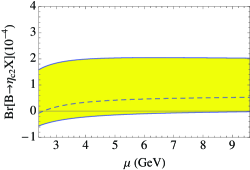
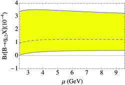
Figure 7: QCD renormalization scale $\mu$-dependence of $Br[B\rightarrow\eta_{c2}X]$ in NDR scheme (left) and HV scheme (right). The long-distance matrix elements are estimated using operator evolution equations. $\mu$ ranges from $\frac{m_{b}}{2}$ to $2m_{b}$. The shaded zone is for the values of $Br[B\rightarrow\eta_{c2}X]$. Upper bound for solid curves correspond to $m_{c}=1.4$ GeV and $\mu_{\Lambda_{0}}=700$ MeV, dashed lines to $m_{c}=1.5$ GeV and $\mu_{\Lambda_{0}}=750$ MeV, and lower bound solid curves to $m_{c}=1.6$ GeV and $\mu_{\Lambda_{0}}=800$ MeV, respectively.

When $\mu$ is taken to be $m_{b}=4.8$ GeV,

$$Br(B\rightarrow\eta_{c2}X)_{NDR} = (\,0.41^{+1.62}_{-0.56}\,)\,\times 10^{-4},$$

$$Br(B\rightarrow\eta_{c2}X)_{HV} = (\,1.24^{+2.23}_{-0.90}\,)\,\times 10^{-4},$$ (53)

where the central values correspond to $m_{c}=1.5$ GeV and $\mu_{\Lambda_{0}}=750$ MeV, upper bounds to $m_{c}=1.4$ GeV and $\mu_{\Lambda_{0}}=700$ MeV, and lower bounds to $m_{c}=1.6$ GeV and $\mu_{\Lambda_{0}}=800$ MeV, respectively. Since the color-octet Wilson coefficient $C_{[8]}(\mu)$ is much larger than the color-singlet one $C_{[1]}(\mu)$

$$\frac{C^{2}_{[8]}(\mu)}{C^{2}_{[1]}(\mu)}\approx 15\,,$$ (54)

the LO decay width is dominated by that of ${}^{1}S_{0}^{[8]}$, which is proportional to $C^{2}_{[8]}(\mu)$. For NLO, decay widths of ${}^{1}S_{0}^{[1]}$ and ${}^{1}D_{2}^{[1]}$ are negligible, and those of ${}^{1}P_{1}^{[8]}$ and ${}^{1}S_{0}^{[8]}$ are of the same order and make most contribution to the branching ratio in Eq. (IV), but unluckily they largely cancel each other. This cancellation is related to our estimates for the long-distance matrix elements in Eq. (IV). If without this cancellation, the ${}^{1}S_{0}^{[8]}$ Fock state could give the following central values

$$Br(B\rightarrow{}^{1}S_{0}^{[8]}X)_{NDR} = \,5.30\,\times 10^{-4},$$

$$Br(B\rightarrow{}^{1}S_{0}^{[8]}X)_{HV} = \,5.45\,\times 10^{-4},$$ (55)

which might be regarded as the upper bound of the branching ratio for this process. Furthermore, we may consider the following uncertainty in the predictions of the branching ratio. Since

$$\frac{C_{[1]}}{C_{[8]}}\sim\alpha_{s}\,,$$ (56)

we might carry out a double expansion in both $\alpha_{s}$ and $C_{[1]}/C_{[8]}$ simultaneously Bergstrom:1994vc . In this new expansion, terms of different orders scale as follows:

LO: $$\quad C^{2}_{[8]}\,;$$

NLO: $$\quad\alpha_{s}C^{2}_{[8]},\;C_{[1]}C_{[8]}\,;$$

N²LO: $$\quad\alpha_{s}^{2}C^{2}_{[8]},\;\alpha_{s}C_{[1]}C_{[8]},\;C^{2}_{[1]}\,;$$

N³LO: $$\quad\alpha_{s}^{3}C^{2}_{[8]},\;\alpha_{s}^{2}C_{[1]}C_{[8]},\;\alpha_{s}C^{2}_{[1]},\cdots\,.$$ (57)

$C^{2}_{[8]}$ scales as LO, and $\alpha_{s}C^{2}_{[8]}$ as NLO. $\alpha_{s}^{2}C^{2}_{[8]}$ scales the same order as $\alpha_{s}C_{[1]}C_{[8]}$ and $C^{2}_{[1]}$, thus should also be considered. Authors of Bergstrom:1994vc did not calculate all $\alpha_{s}^{2}C^{2}_{[8]}$ terms, but estimated their contribution by adding a correction term of the same order. The same method with a minor modification was adopted in Maltoni:1999phd ; Beneke:1998ks . Unluckily, their method can only be applied to the color-singlet channels that have non-vanishing LO decay widths, and fails in our case. In Soares:1997ir the $\alpha_{s}^{2}C^{2}_{[8]}$ virtual contribution from squared one-loop amplitudes was calculated, but the real correction was neglected by arguing that the real contribution was phase-space suppressed. However, the IR divergent real corrections can not be omitted, as pointed out in Maltoni:1999phd ; Beneke:1998ks . Hence, a complete calculation at NNLO in $\alpha_{s}$ might be needed to obtain the $\alpha_{s}^{2}C^{2}_{[8]}$ contribution, but this is already beyond the scope of our calculation in this paper. It will be interesting to see if the large cancellation of ${}^{1}P_{1}^{[8]}$ and ${}^{1}S_{0}^{[8]}$ could be weakened after including the $\alpha_{s}^{2}C^{2}_{[8]}$ contribution.

We now discuss the possible relation between the semi-inclusive decay branching ratio $B\rightarrow\eta_{c2}X$ and the exclusive decay branching ratio $B\rightarrow\eta_{c2}K$. Obviously, the latter must be much smaller than the former, since the $X$ includes many hadronic states other than the kaon. In particular, in the case of $B\rightarrow\eta_{c2}X$, the dominant contribution comes from the color-octet $c\bar{c}$ channels, which subsequently evolve into $\eta_{c2}$ by emitting soft gluons which then turn into light hadrons such as pions. Whereas the exclusive process $B\rightarrow\eta_{c2}K$ requires the soft gluons be reabsorbed by the strange quark in $b\to c\bar{c}+s$. This probability is apparently very small. As a conservative estimate, we believe the branching ratio of $B\rightarrow\eta_{c2}K$ should be smaller than that of $B\rightarrow\eta_{c2}X$ by at least an order of magnitude. The suppression of exclusive decay relative to inclusive decay is supported by many other charmonium states. E.g., the branching ratio of $B\rightarrow J/\psi X$ is $(7.8\pm 0.4)\times 10^{-3}$ Nakamura:2010zzi , while $Br(B^{+}\rightarrow J/\psi K^{+})=(1.014\pm 0.034)\times 10^{-3}$ and $Br(B^{0}\rightarrow J/\psi K^{0})=(8.71\pm 0.32)\times 10^{-4}$. For $\chi_{c1}$, $Br(B\rightarrow\chi_{c1}X)=(3.22\pm 0.25)\times 10^{-3}$, $Br(B^{+}\rightarrow\chi_{c1}K^{+})=(4.6\pm 0.4)\times 10^{-4}$ and $Br(B^{0}\rightarrow\chi_{c1}K^{0})=(3.90\pm 0.33)\times 10^{-4}$. Evidently, the observed inclusive branching ratios are about 10 times larger than the corresponding exclusive one. For $\chi_{c2}$, which is similar to $\eta_{c2}$ because in both cases at LO the color-singlet $c\bar{c}$ Fock states make no contributions, $Br(B\rightarrow\chi_{c2}X)=(1.65\pm 0.31)\times 10^{-3}$, $Br(B^{+}\rightarrow\chi_{c2}K^{+})<1.8\times 10^{-5}$ and $Br(B^{0}\rightarrow\chi_{c2}K^{0})<2.6\times 10^{-5}$, the suppression of exclusive decay is almost by two-order of magnitude. Therefore, we may have a general observation that for a charmonium state produced in B-meson decays, the suppression factor of exclusive production branching ratio relative to inclusive one should not be larger than 1/10 (including the factorizable and non-factorizable exclusive processes). This means $Br(B\rightarrow\eta_{c2}K)$ should be at most $\mathcal{O}(10^{-5})$, based on our calculation.

In contrast, for X(3872) the observed branching ratio $Br(B\rightarrow X(3872)K)\times Br(X(3872)\rightarrow D^{0}\bar{D}^{0}\pi^{0})=(1.2\pm 0.4)\times 10^{-4}$ Nakamura:2010zzi . Considering that there exist many decay modes of X(3872) other than $X(3872)\to D^{0}\bar{D}^{0}\pi^{0}$, we may conclude that $Br(B\rightarrow X(3872)K)$ is at least 10 times larger than $Br(B\rightarrow\eta_{c2}K)$. Therefore, $X(3872)$ is unlikely to be the $J^{PC}=2^{-+}$ charmonium state $\eta_{c2}$. In fact, for X(3872) the $J^{PC}=1^{++}$ assignments of the $D^{0}\bar{D}^{*0}$ moleculeTornqvist:X3872:molecule or a charmonium-$D^{0}\bar{D}^{*0}$ mixed stateMeng:2005er ; Suzuki:2005ha are preferred by many authors, instead of a $J^{PC}=2^{-+}$ state (for more discussions see a recent review Brambilla:2010cs ).

V conclusions

In this paper, we calculate the semi-inclusive decay width and branching ratio of $B\rightarrow\eta_{c2}X$ at NLO in $\alpha_{s}$ in NRQCD factorization framework. The finite short-distance coefficients are obtained by matching QCD and NRQCD, and the non-perturbative long-distance matrix elements are evaluated by using the operator evolution equations. We find that at tree-level, only the S-wave Fock states ${}^{1}S_{0}^{[1,8]}$ contribute, and the LO decay width is dominated by that of ${}^{1}S_{0}^{[8]}$, because of the largeness of the color-octet Wilson coefficient squared $C^{2}_{[8]}(\mu)$ over the color-singlet one $C^{2}_{[1]}(\mu)$. Unlike $\eta_{c2}$ light hadronic decay, in this process, there is no residual divergence at NLO of the ${}^{1}D_{2}^{[1]}$ Fock state, due to the vanishing tree-level contribution of ${}^{1}P_{1}^{[8]}$. At NLO in $\alpha_{s}$, ${}^{1}P_{1}^{[8]}$ and ${}^{1}S_{0}^{[8]}$ dominate. Unfortunately, they largely cancel each other. This cancellation depends on our method for estimating the long-distance matrix elements. As a result, we obtain the branching ratio $Br(B\rightarrow\eta_{c2}X)=(\,0.41^{+1.62}_{-0.56}\,)\,\times 10^{-4}$ in the NDR scheme and $(\,1.24^{+2.23}_{-0.90}\,)\,\times 10^{-4}$ in the HV scheme, at $\mu=m_{b}$. The central values correspond to $m_{c}=1.5$ GeV and $\mu_{\Lambda_{0}}=750$ MeV, upper bounds to $m_{c}=1.4$ GeV and $\mu_{\Lambda_{0}}=700$ MeV, and lower bounds to $m_{c}=1.6$ GeV and $\mu_{\Lambda_{0}}=800$ MeV, respectively. If the large cancellation does not exist, the ${}^{1}S_{0}^{[8]}$ could give $Br(B\rightarrow{}^{1}S_{0}^{[8]}X)_{NDR}=\,5.30\,\times 10^{-4}$ and $Br(B\rightarrow{}^{1}S_{0}^{[8]}X)_{HV}=\,5.45\,\times 10^{-4}$, which could be regarded as the upper bound of the branching ratio of this process. The $\mu$-dependence curves of NLO branching ratios in the two schemes are also shown, where $\mu$ varies from $\frac{m_{b}}{2}$ to $2m_{b}$ and $\mu_{\Lambda}=2m_{c}$. Furthermore, we estimate the exclusive decay branching ratio of $B\rightarrow\eta_{c2}K$ by considering the suppression ratios of exclusive decays relative to inclusive ones for other factorizable and non-factorizable exclusive charmonium production processes, and conclude that $X(3872)$ is unlikely to be a $2^{-+}$ charmonium state. We hope that our results will be useful in finding the missing charmonium state $\eta_{c2}$ in experiments, and in further studying $\eta_{c2}$ production in B-meson exclusive decays.

VI acknowledgments

We would like to thank Yan-Qing Ma and Yu-Jie Zhang for many helpful discussions. This work was supported by the National Natural Science Foundation of China (Nos.10721063, 11021092, 11075002), the Ministry of Science and Technology of China (No.2009CB825200), and the China Postdoctoral Science Foundation (No.2010047010).

VII Appendix

VII.1 Covariant projector method.

In our calculation of short-distance coefficients, the covariant projector method is adoptedKeung:1982jb . For any spin-singlet charmonium production in 4-dimension, the covariant projector is

$$\bar{P}_{0,0}(P,k)=\frac{1}{2\sqrt{2}}\frac{\not{p}_{3}-m_{c}}{\sqrt{\frac{M}{2}+m_{c}}}\gamma^{5}\frac{\not{P}+M}{M}\frac{\not{p}_{4}+m_{c}}{\sqrt{\frac{M}{2}+m_{c}}}\,,$$ (58)

where momentum of charmonium bound state $P=p_{4}+p_{3}$. Relative momentum between charm quark and anti-charm quark satisfies

$$p_{4} = \frac{P}{2}+k,$$

$$p_{3} = \frac{P}{2}-k.$$ (59)

Bound state mass $M=2m_{c}$, which holds in QCD radiative correction calculations, for the relativistic effects are neglected. For more details, one could refer to related contents in Fan:2009cj .

VII.2 One-loop level short-distance coefficients of ${}^{1}S_{0}^{[1]}$, ${}^{1}S_{0}^{[8]}$ and ${}^{1}P_{1}^{[8]}$ Fock states.

For ${}^{1}S_{0}^{[1]}$,

$$g_{1}[{}^{1}S_{0}^{[1]}] = -4(1-\eta)^{2}\left(8\text{Li}_{2}(\eta)-4\text{Z}+4\log(1-\eta)\log(\eta)+\frac{4\pi^{2}}{3}\right)$$

$$+ 20(1-\eta)^{2}+\frac{8(2-5\eta)(1-\eta)^{2}\log(1-\eta)}{\eta}-16\eta(1-\eta)\log(\eta),$$

$$g_{2}[{}^{1}S_{0}^{[1]}] = 4(1-\eta)^{2}\left(3\log\left(\frac{m_{b}^{2}}{\mu^{2}}\right)-\text{X}+\text{Y}\right)-\frac{2\left(17\eta^{2}-53\eta+34\right)(1-\eta)}{2-\eta}$$

$$+ 4\eta^{2}\log(\eta)+\frac{8(3-\eta)(1-\eta)^{3}\log(1-\eta)}{(2-\eta)^{2}},$$

$$g_{3}[{}^{1}S_{0}^{[1]}] = \frac{4}{9}\left(-(1-\eta)\left(2\eta^{2}-7\eta+11\right)-6\log(\eta)\right);$$ (60)

for ${}^{1}S_{0}^{[8]}$,

$$g_{1}[{}^{1}S_{0}^{[8]}] = -\frac{4}{3}(1-\eta)\left(2\eta^{2}-7\eta+11\right)-8\log(\eta),$$

$$g_{2}[{}^{1}S_{0}^{[8]}] = 3(1-\eta)^{2}\left(3\log\left(\frac{m_{b}^{2}}{\mu^{2}}\right)-\text{X}+\text{Y}\right)-\frac{3\left(17\eta^{2}-53\eta+34\right)(1-\eta)}{2(2-\eta)}$$

$$+3\eta^{2}\log(\eta)+\frac{6(3-\eta)(1-\eta)^{3}\log(1-\eta)}{(2-\eta)^{2}},$$

$$g_{3}[{}^{1}S_{0}^{[8]}] = \frac{9}{2}(1-\eta)^{2}\Bigg{(}-4\log\left(\frac{m_{b}^{2}}{\mu^{2}}\right)+\frac{4\text{X}}{3}+\frac{14\text{Y}}{3}-\frac{2\text{Z}}{3}-3\log^{2}(2-\eta)$$ (61)

$$+6\log(1-\eta)\log(2-\eta)-6\log(2)\Bigg{)}+3(1-\eta)\Bigg{(}9(\eta+1)\text{Li}_{2}\left(\frac{1-\eta}{2-\eta}\right)$$

$$-18\text{Li}_{2}\left(\frac{2(1-\eta)}{2-\eta}\right)+(7\eta+29)\text{Li}_{2}(\eta)-\frac{1}{6}\pi^{2}(29\eta+7)$$

$$+18\log(2)\log(2-\eta)+2(4\eta+5)\log(1-\eta)\log(\eta)-18\log(2)\log(\eta)\Bigg{)}$$

$$+\frac{1}{2}\left(90\eta^{2}-48\eta+17\right)\log(\eta)+\frac{\left(20\eta^{3}+2077\eta^{2}-6221\eta+4478\right)(1-\eta)}{12(2-\eta)}$$

$$-\frac{3\left(33\eta^{3}-113\eta^{2}+106\eta+4\right)(1-\eta)^{2}\log(1-\eta)}{(2-\eta)^{2}\eta};$$

and for ${}^{1}P_{1}^{[8]}$,

$$g_{1}[{}^{1}P_{1}^{[8]}] = 16(1-\eta)^{2}\left(2\log(1-\eta)-\log\left(\frac{\mu_{\Lambda}^{2}}{4m_{c}^{2}}\right)\right)-\frac{4}{9}\left(8\eta^{2}-85\eta+119\right)(1-\eta)$$

$$-\frac{8}{3}\left(12\eta^{2}-6\eta+1\right)\log(\eta),$$

$$g_{2}[{}^{1}P_{1}^{[8]}] = 0,$$

$$g_{3}[{}^{1}P_{1}^{[8]}] = 10(1-\eta)^{2}\left(2\log(1-\eta)-\log\left(\frac{\mu_{\Lambda}^{2}}{4m_{c}^{2}}\right)\right)-\frac{1}{9}\left(29\eta^{2}-244\eta+347\right)(1-\eta)$$ (62)

$$-\frac{2}{3}\left(30\eta^{2}-15\eta+7\right)\log(\eta).$$

References

• (1) E. J. Eichten, K. Lane, C. Quigg, Phys. Rev.  D69, 094019 (2004). [hep-ph/0401210].
• (2) T. Barnes, S. Godfrey, E. S. Swanson, Phys. Rev.  D72, 054026 (2005). [hep-ph/0505002].
• (3) B. -Q. Li, K. -T. Chao, Phys. Rev.  D79, 094004 (2009). [arXiv:0903.5506 [hep-ph]].
• (4) Y. Fan, Z. -G. He, Y. -Q. Ma, K. -T. Chao, Phys. Rev.  D80, 014001 (2009). [arXiv:0903.4572 [hep-ph]].
• (5) G. T. Bodwin, E. Braaten and G. P. Lepage, Phys. Rev.  D 51, 1125 (1995) [Erratum-ibid.  D 55, 5853 (1997)] [arXiv:hep-ph/9407339].
• (6) H. -w. Huang, K. -t. Chao, Phys. Rev.  D54, 3065-3072 (1996); Erratum-ibid. D56, 7472–7472 (1997); Erratum-ibid. D60, 079901(E) (1999). [hep-ph/9601283].
• (7) H. -W. Huang, K. -T. Chao, Phys. Rev.  D55, 244-248 (1997). [hep-ph/9605362].
• (8) H. -W. Huang, K. -T. Chao, Phys. Rev.  D54, 6850-6854 (1996); D56, 1821 (E) (1997). [hep-ph/9606220].
• (9) A. Petrelli, M. Cacciari, M. Greco, F. Maltoni, M. L. Mangano, Nucl. Phys.  B514, 245-309 (1998). [hep-ph/9707223].
• (10) F. Maltoni, PhD thesis, University of Pisa, 1999, http://maltoni.web.cern.ch/maltoni/.
• (11) Z. -G. He, Y. Fan, K. -T. Chao, Phys. Rev. Lett.  101, 112001 (2008). [arXiv:0802.1849 [hep-ph]].
• (12) Z. -G. He, Y. Fan, K. -T. Chao, Phys. Rev.  D81, 074032 (2010). [arXiv:0910.3939 [hep-ph]].
• (13) K. Nakamura et al. [Particle Data Group], J. Phys. G 37, 075021 (2010).
• (14) M. Beneke, F. Maltoni, I. Z. Rothstein, Phys. Rev.  D59, 054003 (1999). [hep-ph/9808360].
• (15) L. Bergstrom, P. Ernstrom, Phys. Lett.  B328, 153-161 (1994). [hep-ph/9402325].
• (16) P. Ko, J. Lee, H. S. Song, Phys. Rev.  D53, 1409-1415 (1996). [hep-ph/9510202].
• (17) S. Fleming, O. F. Hernandez, I. Maksymyk, H. Nadeau, Phys. Rev.  D55, 4098-4104 (1997). [hep-ph/9608413].
• (18) J. M. Soares, T. Torma, Phys. Rev.  D56, 1632-1637 (1997). [hep-ph/9702420].
• (19) F. Yuan, C. F. Qiao and K. T. Chao, Phys. Rev.  D 56, 329 (1997) [arXiv:hep-ph/9701250].
• (20) P. Ko, J. Lee, and H.S. Song, Phys. Lett. B 395, 107 (1997) [arXiv:hep-ph/9701235].
• (21) Y. J. Zhang, Y. J. Gao and K. T. Chao, Phys. Rev. Lett.  96, 092001 (2006); Y. J. Zhang and K. T. Chao, Phys. Rev. Lett.  98, 092003 (2007); Y. Q. Ma, Y. J. Zhang, and K. T. Chao, Phys. Rev. Lett. 102, 162002 (2009); B. Gong and J. X. Wang, Phys. Rev. Lett. 102, 162003 (2009); Y. J. Zhang, Y. Q. Ma, K. Wang, and K. T. Chao, Phys. Rev. D 81, 034015 (2010).
• (22) J. Campbell, F. Maltoni, F. Tramontano, Phys. Rev. Lett. 98, 252002 (2007); P. Artoisenet, J. Campbell, J.P. Lansberg, F. Maltoni, F. Tramontano, Phys.Rev.Lett.101, 152001 (2008); B. Gong and J. X. Wang, Phys. Rev. Lett.  100, 232001 (2008), Phys. Rev. D77, 054028 (2008).
• (23) Y. Q. Ma, K. Wang, and K. T. Chao, Phys. Rev. Lett. 106, 042002 (2011), Phys. Rev. D84, 114001 (2011); Y. Q. Ma, K. Wang, and K. T. Chao, Phys. Rev. D 83, 111503(R) (2011); M. Butenschoen and B. A. Kniehl, Phys. Rev. Lett. 106, 022003 (2011); M. Butenschoen and B. A. Kniehl, AIP Conf. Proc. 1343, 409 (2011).
• (24) P. Artoisenet, J. M. Campbell, F. Maltoni, and F. Tramontano, Phys. Rev. Lett. 102, 142001 (2009); C. H. Chang, R. Li, and J. X. Wang, Phys. Rev. D 80, 034020 (2009); M. Butenschoen and B. A. Kniehl, Phys. Rev. Lett. 104, 072001 (2010).
• (25) P. del Amo Sanchez et al. [BABAR Collaboration], Phys. Rev.  D 82, 011101 (2010) [arXiv:1005.5190 [hep-ex]].
• (26) Y. Jia, W. L. Sang and J. Xu, arXiv:1007.4541 [hep-ph].
• (27) T. J. Burns, F. Piccinini, A. D. Polosa and C. Sabelli, Phys. Rev.  D 82, 074003 (2010) [arXiv:1008.0018 [hep-ph]].
• (28) Yu. S. Kalashnikova and A. V. Nefediev, Phys. Rev.  D 82, 097502 (2010) [arXiv:1008.2895 [hep-ph]].
• (29) H.W. Ke and X.Q. Li, Phys. Rev. D 84, 114026 (2011) [arXiv:1107.0443].
• (30) T. Mehen and R. Springer, Phys. Rev.  D 83, 094009 (2011) [arXiv:1101.5175 [hep-ph]].
• (31) G. Buchalla, A. J. Buras, M. E. Lautenbacher, Rev. Mod. Phys.  68, 1125-1144 (1996). [hep-ph/9512380].
• (32) E. Braaten, J. Lee, Phys. Rev.  D67, 054007 (2003). [hep-ph/0211085].
• (33) Y. Fan, ”Estimate of the $h_{c}$ decay width in NRQCD”, talk at Topical Seminar on Frontier of Particle Physics 2010: Charm and Charmonium Physics, Hu Yu Village, Beijing, August 27, 2010. http://indico.ihep.ac.cn/conferenceTimeTable.py?confId=1484
• (34) E. J. Eichten and C. Quigg, Phys. Rev.  D 52, 1726 (1995) [arXiv:hep-ph/9503356].
• (35) A. J. Buras and P. H. Weisz, Nucl. Phys.  B 333, 66 (1990).
• (36) G. Altarelli, S. Petrarca, Phys. Lett.  B261, 303-310 (1991).
• (37) C. S. Kim, A. D. Martin, Phys. Lett.  B225, 186 (1989).
• (38) E.S. Swanson, Phys. Lett. B 588, 189 (2004); 598, 197 ( 2004); N.A. Tornqvist, Phys. Lett. B 590, 209 (2004); F. Close and P. Page, Phys. Lett. B 578, 119 (2004); C.Y. Wong, Phys. Rev. C 69, 055202 (2004); E. Braaten and M. Kusunoki Phys. Rev. D 69, 074005 (2004); M.B. Voloshin, Phys. Lett. B 579, 316 (2004).
• (39) C. Meng, Y. J. Gao and K. T. Chao, arXiv:hep-ph/0506222.
• (40) M. Suzuki, Phys. Rev.  D 72, 114013 (2005) [arXiv:hep-ph/0508258].
• (41) N. Brambilla et al., Eur. Phys. J.  C71, 1534 (2011). [arXiv:1010.5827 [hep-ph]].
• (42) W. -Y. Keung, I. J. Muzinich, Phys. Rev.  D27, 1518 (1983).