Present address: ]University of Victoria, Victoria, British Columbia.
Present address: ]University of Glasgow, Glasgow, United Kingdom.
Present address: ]JINR, Dubna, Russia
Present address: ]Fermi National Accelerator Laboratory, Ilinois 60510, USA.
Present address: ]AECL, Mississauga, Ontario, Canada.
Affiliated with: ]University of Victoria, Victoria, British Columbia, Canada.
Affiliated with: ]University of Saskatchewan, Saskatoon, Saskatchewan, Canada.
TWIST Collaboration
Precision muon decay measurements and improved constraints on the weak interaction
Abstract
The TWIST Collaboration has completed its measurement of the three muon decay parameters , , and . This paper describes our determination of , which governs the shape of the overall momentum spectrum, and , which controls the momentum dependence of the parity-violating decay asymmetry. The results are and . These are consistent with the value of given for both parameters in the standard model, and each is over a factor of 10 more precise than the measurements published prior to TWIST. Our final results on , , and have been incorporated into a new global analysis of all available muon decay data, resulting in improved model-independent constraints on the possible weak interactions of right-handed particles.
pacs:
13.35.Bv, 14.60.Ef, 12.60.CnI Introduction
The TWIST experiment is a high-precision search for evidence of contributions to the charged-current weak interaction beyond those described by the standard model (SM) of particle physics. We take advantage of the purely leptonic nature of the decay of the positive muon into a positron and two neutrinos, , which can be described to a good approximation as a four-fermion point interaction and in the SM is mediated by the boson.
The most general Lorentz-invariant, local, and lepton-number-conserving description is given by the matrix element
| (1) |
where each scalar (), vector (), or tensor () interaction between -handed muons and -handed positrons has an associated coupling constant satisfying certain normalizations and constraints Fetscher:1986 . Only 19 real and independent coupling constants are needed to describe entirely the interaction because and , and a common phase is not observable. In the context of the interaction of the SM, all coupling constants are zero except for . The coupling constants provide the probability for a -handed muon to decay into an -handed positron using
| (2) |
where for and for . In particular, a model-independent limit on any muon right-handed couplings Fetscher:1986 ; PDG is determined from the probability
| (3) |
The differential muon decay spectrum Michel50 , using the notation of Fetscher and Gerber PDG , can be written as
| (4) | |||||
where is the Fermi coupling constant, is the angle between the muon spin and the positron momentum, MeV is the kinematic maximum positron energy, is the positron’s reduced energy, is the minimum possible value of , corresponding to a positron of mass at rest, and is the degree of muon polarization at the time of decay. is typically reduced from , which is the helicity of the muon at the time of its production from a pion decay, due to depolarization undergone by the muon before it decays.
The isotropic and anisotropic parts of the spectrum
| (5) | |||||
| (6) | |||||
are parametrized by four muon decay parameters , , , and , which are bilinear combinations of the coupling constants . These four parameters, with the addition of the radiative corrections and , are sufficient to describe the shape of the momentum-angle spectrum of the decay positron. We analyze the momentum-angle spectrum rather than the energy-angle spectrum out of convenience and because for these energies the difference is insignificant.
The introduction of chiral spin 1 fields to the SM has been investigated Chizhov94 ; Chizhov_Review . One consequence is that nonlocal tensor interactions appear, so that and are no longer zero. These new couplings can be measured in particular through the parameter.
Initial and intermediate measurements of and have already been published musser:2005 ; gaponenko:2005 ; Robpaper . This paper presents a detailed description of the final measurement of the and decay parameters by the TWIST Collaboration reported in mischke:2011 . An identical and simultaneous analysis of the same data yielded the final parameter determination; a complete description with an emphasis on the systematic uncertainties specific to was presented in Jamespmuxi . The decay parameter was fixed to the global analysis value of gagliardi:2005 because the sensitivity to this parameter is reduced due to the multiplying factor .
II Experimental setup
II.1 TWIST spectrometer
A brief description of the experimental setup is given here. A more detailed description of the apparatus can be found in TWIST_Apparatus:2005 with the improvements made for this final analysis described in Jamespmuxi .
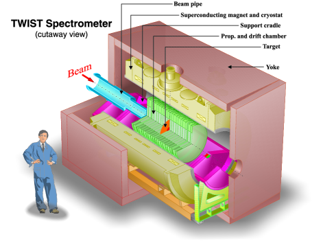
An overview of the TWIST apparatus is shown in Fig. 1; it was installed on the M13 beamline at TRIUMF, Vancouver, Canada. The 500 MeV proton beam from the TRIUMF cyclotron hit a carbon target producing pions, some of which stopped and decayed near the surface of the target to create 29.79 MeV/ muons with 100% polarization. The beamline was tuned to transport these highly polarized muons with a central momentum of 29.6 MeV/ and a momentum bite of 0.7% FWHM. The beam also contained several times as many positrons as muons, with the ratio varying with different tuning conditions. After passing through the beamline, the muons stopped at a rate between 2000 s-1 and 5000 s-1 in a thin target foil located in the center of the highly symmetric array of 44 planar drift chambers (DCs) Davydov and 12 planar proportional chambers (PCs) composing the TWIST detector (Fig. 2). The DCs and the PCs had an active region of 32 cm diameter and contained respectively 80 and 160 parallel sense wires separated by 0.4 cm and 0.2 cm.
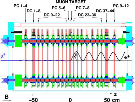
The DCs were filled with dimethyl ether gas and were assembled in modules of two or eight chambers in which the aluminized Mylar cathode foils were shared by neighboring chambers. DC 9-22 and 23-36, installed in two-chamber modules, formed a sparse stack covering most of the tracking region. The two eight-chamber DC 1-8 and 37-44 modules instrumented the end of the tracking region Jamespmuxi . PC 1-4 and 9-12 were installed at the ends of the detector for particle identification purposes. The PC 5-8 module had the target foil as central cathode foil and was installed in the center of the detector stack to make the entire array symmetric. The PCs were filled with a mixture of CF4 and isobutane. The array of low mass chambers was installed in a frame referred to as the cradle, filled with helium to further reduce the amount of material traversed by the muons and positrons. Two different target foils were used over two run periods to study the effects of the target material on the decay parameters measurement: a (30.9 0.6) m thick silver foil and the (71.6 0.5) m thick aluminum foil used for the intermediate TWIST measurement Robpaper . Both metal targets had purity exceeding 99.999% and featured minimal depolarization of the muons after stopping JamesPRB .
The detector was installed in a superconducting solenoid producing a magnetic field of 2 T that was highly uniform over the tracking region and aligned with the beam direction. In order to obtain the required field uniformity and also to reduce fringe fields, it was necessary to surround the solenoid cryostat with a cube-shaped yoke of approximately 3 m on a side. Two NMR probes were installed slightly beyond the radius of the tracking region in the cradle to monitor constantly the magnetic field strength during data taking.
The magnetic field was mapped using a rotating arm equipped with Hall probes to measure the longitudinal component with a precision of 0.1 mT and an NMR probe for the total field. The Hall probes were separated by about 4.13 cm on the arm. A full rotation was performed every 5.0 cm along for the central part of the tracking region, and every 2.5 cm for the edges of the region. The tracking region was fully mapped for each of the three field strengths used during data taking, 1.96 T, 2.00 T, and 2.04 T. A smooth and higher granularity field map, including the relatively small transverse field components, was calculated using the Opera-3D software opera , matching the measured magnetic field map within 0.2 mT over the drift chamber region.
The beamline vacuum pipe was extended through the fringe field region as close as possible to the end of the detector array. Upon exit from the vacuum, muons passed through elements of a “beam package,” including a 20 cm length of gas degrader filled with an adjustable mixture of He and CO2 gas, a film strip degrader, and a muon scintillator that triggered the data acquisition system. The film strip degrader consisted of a roll of plastic film containing holes covered with Mylar degraders of varying thicknesses up to 0.1 cm. It could be rolled from outside the magnet yoke to choose which degrader was in the muon path. It was used to significantly degrade the muon beam momentum in order to stop muons well upstream of the target at the detector center, for special runs used for positron interaction studies (Sec. IV.1). The film degrader was set to an empty hole of the film strip for the normal acquisition of muon decay data. The muons traversed a total of 140 mg/cm2 of material, including the beam package and the upstream half of the detector, before stopping in the target. The transverse size of the beam spot was 1.6 cm FWHM. Because the chambers were operated at atmospheric pressure and thus the gas density varied with time, the ratio between the two gases in the gas degrader was automatically changed by a feedback loop to set and maintain the muon stopping distribution in the target.
The downstream end of the detector was equipped with a second beam package during one data set to test the impact on the data of the asymmetry due to the presence of the upstream beam package. Two removable time expansion chambers (TECs) were installed in the beam in the upstream fringe field region at the beginning and the end of each data set to characterize the muon beam properties Hu:2006 .
II.2 Experimental data
The data used for the final phase were taken during fall 2006 for the Ag target and in summer 2007 for the Al target (see Tables 1 and 2; the numbering of sets is not necessarily sequential). Monitor information was recorded during all runs for variables such as spectrometer temperatures, gas pressures and flows, and muon beamline element settings, and was later evaluated to identify any instabilities that could signify a low quality of data. Approximately 10% to 30% of runs in each set were discarded prior to the analysis to guarantee stable run conditions during the period of typically one week necessary to take a set. The criteria for rejection were conservative and unbiased; for example, they identified runs with a problem in the data acquisition system, runs with a noisy chamber, or runs before the gas degrader feedback loop was fully locked.
The four nominal sets 74, 75, 84 and 87 were taken with optimal conditions for the measurement of decay parameters. For set 68, the degrader was changed so that the center of the muon stopping distribution was moved from near the middle of the target to a point only 1/3 of the way through, to determine the sensitivity to stopping position variations. Set 83 was taken with a downstream beam package mirroring the upstream beam package to test the impact of the positrons backscattering into the spectrometer and the consistency of the results with or without a symmetric apparatus. Two sets (70 and 71) were taken with different solenoid magnetic field strengths to verify that the decay parameters are insensitive to the transverse scale of the helices.
Set 72 was unique in that it was taken with the TECs in place in the beamline, in order to test the effects of extra multiple scattering of the muon beam on the parameter through the depolarization of the muons, and also to monitor the stability of the muon beam position and angle over an entire week. The muon beam was steered off the detector axis with an angle 30 mrad for set 76 and with a position -1 cm and an angle -10 mrad for set 86 to study the depolarization in the fringe field in simulation. Sets 70, 71, 72, 76 and 86 were discarded from the measurement and used for systematic uncertainties studies due to their large depolarization uncertainties Jamespmuxi , but were used for and since these parameters are insensitive to the muon polarization.
The M13 central momentum was reduced to 28.75 MeV/ for set 91 and to 28.85 MeV/ for sets 92-93 to study the effect of multiple scattering of the muons exiting the production target. The muons were stopped at the entrance of the detector for sets 73 and 80 by changing the momentum selection and introducing a film degrader in the beamline. These special sets of data are used to validate the simulation (Sec. IV).
| Data | Description | Events () | |
|---|---|---|---|
| set | |||
| Before | Final | ||
| cuts | spectrum | ||
| 68 | Bragg peak | 741 | 32 |
| into target | |||
| 70 | Central field at 1.96 T | 952 | 50 |
| 71 | Central field at 2.04 T | 879 | 45 |
| 72 | TECs in place, nominal beam | 926 | 49 |
| 73 | Muons stopped at detector entrance | 1113 | |
| 74 | Nominal | 580 | 32 |
| 75 | Nominal | 834 | 49 |
| 76 | Off-axis beam | 685 | 39 |
| Data | Description | Events () | |
|---|---|---|---|
| set | |||
| Before | Final | ||
| cuts | spectrum | ||
| 80 | Muons stopped at | 363 | |
| detector entrance | |||
| 83 | Downstream beam package in place | 943 | 49 |
| 84 | Nominal | 1029 | 43 |
| 86 | Off-axis beam | 1099 | 58 |
| 87 | Nominal | 854 | 45 |
| 91 | Lower momentum I | 225 | 11 |
| 92 | Lower momentum II | 322 | 15 |
| 93 | Lower momentum III | 503 | 26 |
III Analysis
The muon decay parameters are extracted from the momentum-angle (-) spectrum of the decay positrons measured in the TWIST spectrometer. More precisely the difference in shape between the - spectra from the data and from a full simulation of the TWIST apparatus is interpreted in terms of a difference in decay parameters. A blind analysis is performed by using hidden decay parameters for the generation of the simulation AndreiPhD . These parameters remain hidden until the end of the analysis when all systematic uncertainties and corrections have been determined to minimize the possibility that the results are affected by human bias.
The simulation is analyzed using the same reconstruction and event selection that is applied to the data, and reproduces very closely the detector response. Differences between data and simulation arise from differences in the muon decay parameters and radiative corrections, and additionally from uncertainties in the simulation inputs. The latter are the source of most of the systematic uncertainties.
III.1 Simulation
The Monte Carlo simulation of the TWIST experiment uses the geant 3.21 package Geant321 to simulate the particle interactions, the detector geometry, and its electronics. None of the physics processes undergone by the particles such as bremsstrahlung or -electron production are modified or tuned from their definitions in geant 3.21. Since our apparatus had very thin scattering layers, for the energy loss we used the optional simulation of reduced Landau fluctuations with delta rays.
The simulation includes all the elements necessary to reproduce accurately the muon and positron trajectories. The particles are transported in the Opera-3D magnetic field map using a classical fourth order Runge-Kutta numerical method. The description of the wire chambers includes the cathode planes and the wires, as well as their positions measured by the alignment calibration (Sec. III.6). The discontinuous behavior of the ionization of the wire chamber gas is simulated with ionization clusters generated randomly along the path of the charged particles. The ion cluster separation is matched to the data by comparing the timing of hits close to the wire in data and simulation. The drift time of each cluster is calculated from DC space-time relations (STRs) created by a Garfield simulation Garfield of the DCs. The effect of regions of the sense wires becoming temporarily inefficient due to the presence of ionization from previous muon hits is also simulated. The data acquisition digitization is part of the simulation in order to have output identical in format to that of the apparatus.
For each data set, a corresponding simulation is generated with its input parameters matched to the specific data taking conditions for that set, as needed. The fractions of He and CO2 in the gas degrader are set to time averaged values from the data. The muon beam profile measured by the TECs is used to generate the initial muon directions Jamespmuxi . The muon and positron beam rates are matched to the data to simulate accurately the overlap in time of the hits in the DCs. Pions and cloud muons111Cloud muons originate from pions decaying in flight as they move from the production target to the M13 beamline. These muons have a low polarization and are therefore removed during the analysis of the data with a time of flight cut. are beam particles that are not simulated because they can be effectively eliminated from the experimental data. The magnetic field strength is matched to the cradle NMR probe measurements performed during each data set. Energy loss in some components outside of the tracking region is also simulated. For example, the upstream beam package had to be simulated in detail to reproduce the positrons scattering back into the detector and affecting the track reconstruction. The entire downstream beam package was also included in the simulation matching set 83.
Individual muons are generated at the location of the TECs, where the real beam has been well characterized, with polarization of 100% in a direction opposite to their momentum. The initial momentum and angle of the decay positron are generated with an independent program in order to isolate the hidden parameters of the blind analysis. The hidden parameters are chosen randomly within a range of from the SM values and remain encrypted during the whole analysis. The algorithm uses an accept-reject Monte Carlo technique with the theoretical - spectrum including full radiative corrections with exact electron mass dependence, the leading logarithmic terms of , the next-to-leading logarithmic terms of , leading logarithmic terms of , correction for soft pairs and virtual pairs, and an ad-hoc exponentiation Arbuzov . The boson’s mass and the strong interaction contributions to the decay through loops are respectively on the order of and Davydychev et al. (2001), orders of magnitude smaller than our precision goal, and are therefore ignored for this measurement.
III.2 Event and track reconstruction
The reconstruction software is composed of three main algorithms. It begins by grouping the hits in the spectrometer into different time windows and by identifying the type of particle (e.g., decay positron, beam positron, incident muon, secondary electron, etc.) causing the hits. Then a pattern recognition algorithm uses the positions of the hit wires to define helical tracks within each time window, using spatial information to separate the hits from two particles completely overlapped in time if necessary. Electron and positron tracks are finally reconstructed with high precision using the drift information in the DCs to extract the momentum and direction of the particles.
Information from a 16 s interval is recorded for each event (from 6 s before to 10 s after the muon trigger) and divided into time windows designed to group together the signals coming from each particle. The signals from the PCs define the beginning of the time windows because their time resolution is ns. The time windows are by default 1050 ns long to include the longest drift times in the DCs (50 ns before and 1000 ns after the first PC hit time). However if two particles are separated in time by less than 1000 ns but more than 100 ns, the first time window stops at the beginning of the second window. This type of event is rejected later in the analysis because signals of the particle in the first window can end up in the second window, confusing the track reconstruction. On the other hand, a time separation of less than 100 ns is not considered long enough for the PCs to identify two different particles and only one time window is created. In this case the signals corresponding to each particle are separated by the pattern recognition using spatial information. This topology also includes the backscatter of a decay positron from material outside the tracking region creating two independent tracks overlapping in time, as well as delta rays emitted in the tracking region.
The particle identification algorithm uses the pulse widths in the PCs, roughly proportional to the energy deposited, to separate muons from positrons since the two particles deposit different amounts of energy. Beam positrons are identified using the fact that they traverse the entire detector while the decay positrons originate from the target foil region in the middle of the chamber stack. The events are classified according to the particle content and the length of the time windows.
The track reconstruction algorithm is performed on the signals in each time window. The first part of this algorithm is a pattern recognition, which combines hits on adjacent wires and associates signals together to form a coarse estimate of the helical track. The drift times are ignored at this stage and for this reason the Chebyshev norm is used as a fit optimizer F_James . This pattern recognition identifies and separates the tracks from the different particles contained in a time window, including -ray electrons. A particle undergoing a large enough scattering or energy loss due to the emission of a bremsstrahlung photon or a -ray electron is reconstructed as two individual tracks by the algorithm.
The next stage of the track reconstruction uses a minimization to refine the helical trajectory identified by the pattern recognition. This helix fitter minimizes the residuals at each DC plane as well as kink angles in the center of each DC module, and includes as a fit parameter the decay time of the muon. The time of flight of the decay positron to each DC plane is included in this calculation. The kink approach is well adapted to the TWIST spectrometer since the scattering masses are discrete Lutz . The kink angles are weighted in the minimization by the inverse of the width of the Gaussian approximation calculated using the formula for multiple scattering through small angles PDG Thru Matter . For this analysis the space-time relationships used to convert the drift times into drift distances were measured using decay positron tracks (see Sec. III.6). The trajectories between the DCs are calculated using the Opera-3D magnetic field map to account for the inhomogeneities of the solenoid magnetic field. The algorithm uses an arc step approximation with variable size steps to integrate the magnetic field features. The energy lost by the positron through ionization is taken into account in the fitting procedure using
| (7) |
with the average energy loss of a track segment, the thickness of the material , and the ionization energy lost per unit of thickness in the material calculated from the mean energy loss formulas PDG Thru Matter . The track reconstruction has an inefficiency of a few , and an angle-dependent resolution at the end point (52.8 MeV/), which is 58 keV/ when extrapolated to . From simulation, the absolute accuracy of the reconstructed momentum is better than .
III.3 Event selection
It is desirable to select classes of events that are very simple and therefore well simulated to reduce discrepancies between data and simulation. Our main selection is to find one muon and one decay positron separated by more than 1 s. Events also containing a beam positron are kept only if the beam particle is separated from the incident muon and decay positron by more than 1 s or less than 100 ns. A track from a decay positron backscattering at the upstream end of the detector and a beam positron track are indiscernible by the particle identification. The backscattering depends strongly on the decay positron momentum and angle. Thus events with a backscattered positron and events with overlap of decay and beam positrons within 100 ns are included in the analysis. These choices reduce the sensitivity of the analysis to the accuracy in the simulation of these processes.
The highly polarized surface muons are selected using time of flight of the particles in the M13 beamline Jamespmuxi . A highly polarized muon beam is crucial for the measurement of , but also increases the sensitivity to the parameter. The muons stopping in the target foil are selected by the next series of cuts. The first PC downstream and adjacent to the target acts as a veto for muons stopping too far downstream. The pulse widths in the two PCs just upstream of the target are used to eliminate muons that stopped in the gas or the wires of those chambers Jamespmuxi . Also the muon position on the target measured by the two PCs upstream is used to reject muons stopping more than 2.5 cm away from the central axis of the detector. Decay positrons from these rejected muons might not be contained within the tracking region.
The purpose of the following selections is to identify which track corresponds to the decay positron. Tracks that failed the second stage of the track reconstruction and tracks corresponding to negatively charged particles are rejected. The event classification determined on which side of the target the decay positron was emitted based on the side containing most of the hits. Tracks located on the opposite side are discarded. The next selection tries to match together tracks to check whether they originated from the same particle. In particular, the algorithm tries to match tracks from opposite sides of the target (using previously discarded tracks) to identify beam positron tracks and remove them from the analysis. In this case the criteria for a match are a time separation of less than 60 ns for the track times and a closest distance of approach of the two extrapolations of the tracks of less than 0.5 cm. The matching can also identify trajectories split in two tracks (both located on one side of the target) due to a large scattering in a DC. In this case the closest distance of approach is only required to be 2 cm. The position at the target of the muon as measured by the target PCs is compared to the extrapolation of the positron track back to the target to determine the vertex distance. An angle-dependent cut is applied to this vertex distance. If more than one track candidate was selected, two more selections determine a single track corresponding to the decay positron. The tracks that are farthest from the target plane are discarded. If multiple tracks are equally close to target, the selected track candidate is the one with the shortest muon-positron vertex distance. Finally only the decays happening between 1050 ns and 9000 ns are selected. Earlier tracks might overlap with DC signals from the muon. DC signals from later tracks may occur after the end of the event recording.
It is important to recall that exactly the same algorithms are applied to data and simulation, reducing the dependence of our muon decay results on the precision of the algorithms. The evaluation of the systematic uncertainties from the detector response is accomplished using event selection criteria identical to that of the analysis, and therefore integrates the effect of the cuts in the uncertainties (Sec. V).
III.4 Muon decay parameter fit
The - spectra obtained for data and simulation are now compared to perform a momentum calibration and to extract their difference in terms of decay parameters. The data and simulation spectra have very different muon decay parameters, compared to the precision of the measurement, because of the hidden parameters in simulation. This difference is typically a few parts in and it biases the edge fit of the momentum calibration performed at the kinematic end-point of the two spectra. The shape of the spectrum near the end-point is sensitive to this difference, so it is necessary to include in the simulation the derivatives weighted according to the results from a prior decay parameter fit. For this reason the two fitting procedures are applied iteratively, starting with the decay parameter fit. Only one iteration of the momentum calibration is needed to reach convergence.
The muon decay parameter fit procedure exploits the linearity in the decay parameters , and the products and [Eq. (4)]. The difference between the data spectrum () and the Monte Carlo simulation spectrum () can be expressed in terms of derivative spectra of the decay parameters AndreiPhD . Schematically:
| (8) | |||||
where the are the free parameters of the fit. The effect of the detector response on the - derivative spectra is simulated using the same code as is used for the muon decay spectrum. However, unlike the decay spectrum, the derivatives are not positive definite, and additional sign information must be passed to the fitting software. The radiative corrections are already taken into account in the simulation.
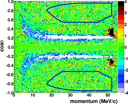
Fiducial regions in the - spectrum are defined to reduce bias while maximizing resolution and sensitivities to the decay parameters. Only the bins whose center is contained in the fiducial regions are used in the decay parameters fit. The maximum momentum cut () avoided the region of the spectrum that was used in a momentum calibration procedure (described below). The longitudinal momentum cut () avoided the region where the helix wavelength was difficult to determine. The requirement removed small angle tracks where the wavelength was poorly resolved, and eliminated large angle tracks with less reliable reconstruction due to multiple Coulomb scattering as the path length through the chambers became too large. The maximum transverse momentum cut () retained only the positrons within the instrumented regions of the detector. The minimum transverse momentum cut () removed tracks where the helix radius became comparable to the wire spacing. The upstream and downstream fiducial regions are symmetric about (Fig. 3). We studied the stability of the decay parameters with respect to the definition of the regions by varying by a few percent all the fiducial boundaries. These boundaries were slightly modified for this analysis compared to the ones used for the intermediate measurement Robpaper .
A minimization, using MINUIT MINUIT , of Eq. (8) to the data is used to determine the muon decay parameter differences. The correlations between the parameters as returned by the fitting algorithm are 0.19 for -, 0.21 for - and for -. The parameter is not part of the fit in this analysis because it is strongly correlated to the parameters and (Sec. I) and the fiducial regions exclude the low momentum part of the spectrum, which is the most sensitive to this parameter. The final determination of from is only possible using the hidden parameters and in the formula:
| (9) |
However, before unblinding it is sufficient to use the SM values to estimate . The final value of is recalculated after the hidden parameters have been revealed.
III.5 Momentum calibration
The momentum calibration exploits the kinematic end-point of the decay positron momentum at 52.83 MeV/ to measure the mismatch between the data and simulation detector responses. Because the planar geometry of the TWIST detector, the momentum loss of the positrons exiting the target will have a dependence. Histograms of the edge region with 10 keV/ momentum binning and bins in of width 0.0636 in the range () are produced. For each slice the simulated edge histogram is shifted in 10 keV/ steps with respect to the data histogram. At each step a statistic is calculated using the difference in bin contents between the spectra. The resulting distribution is fitted with a second-order polynomial to determine the momentum shift required to minimize the . The momentum mismatch between data and simulation versus (see Fig. 4) is fitted independently upstream and downstream with straight lines,
| (10) |
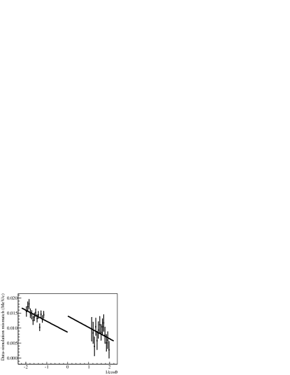
A new data - spectrum is produced by applying the momentum calibration for each set on an event-by-event basis, and the statistical uncertainties and correlations of the calibration parameters are propagated to the muon decay parameter error budget. Table 3 shows the mean values of the momentum calibration parameters.
| Target | ||||
|---|---|---|---|---|
| keV/ | keV/ | keV/ | keV/ | |
| Ag | 1.8 0.5 | -10.0 0.8 | -3.1 1.3 | -1.7 2.0 |
| Al | 4.8 0.6 | -6.9 0.9 | -0.2 1.4 | -11.0 2.3 |
The model used for the propagation of the momentum mismatch to the entire spectrum depends on the source or sources of the mismatch, which could not be uniquely identified. For this reason the final muon decay parameter results are the average of the analyses calibrated using a shift that was either constant or scaled with momentum. Systematic uncertainties associated with the momentum calibration are discussed in Sec. V.3.
III.6 Drift chamber calibration
Improvements to the DC calibration procedures have been crucial to reach our final precision for the decay parameters. First of all the wire time offsets, which correct for the different propagation times of the signals from different sense wires, were measured directly from the decay positrons in the physics data. Previously the wire time offsets were determined from special pion data taken only at the beginning and the end of run periods, leading to a dominant systematic uncertainty from the time dependence of these offsets. For this measurement, a downstream scintillator was used in addition to the existing upstream scintillator. Both scintillators recorded the arrival time of the decay positron as a reference. The upstream scintillator is an annular shaped positron scintillator installed around the main muon trigger scintillator. The downstream scintillator on the other hand is installed outside of the steel yoke and covers most of the yoke downstream opening.
The wire time offsets were extracted from the decay positron signals after a time of flight correction. The algorithm for fitting these time distributions, which are broadened by the drift times of the electrons in the DCs, was significantly improved. The mismatch of the offsets between data and simulation was estimated to be less than 0.5 ns channel-by-channel based on the difference in the fit parameter describing the steepness of the DC signal rising edge.
The relative misalignment of the DCs was measured and corrected in the analysis to improve the reconstruction resolution. A special set of data was taken with 120 MeV/ pions and with no magnetic field. The straight tracks produced by the pions traveling through the entire chamber stack were reconstructed. At each wire chamber, the residuals were used in an iterative process to determine the misalignment in translation in the direction measured by the chamber (perpendicular to the wires) and in rotation around the detector axis with a precision respectively of 10 m and 0.03 mrad. The target PCs misalignment was also corrected due to their importance to measure the muon-positron vertex distance. The misalignment between the spectrometer and the magnetic field axis was measured on muon decay data using a special helix fitting algorithm allowing for a rotated helix axis. This measurement was performed 3 times, each time that the spectrometer was removed from inside the coils. The three misalignments showed remarkable reproducibility, being consistent within the 0.03 mrad uncertainty, with an average value of 0.31 mrad in and 1.15 mrad in .
The previous TWIST analyses used STRs extracted from Garfield simulations. This analysis measured effective STRs independently for both simulated and real data from the time residuals of the helix fitter on decay positron tracks AlexNIM . An iterative procedure modified the STRs to reduce the time residuals in subcells of the drift cell surrounding the sense wire. All the drift cells are averaged for each plane. The main advantages of the new procedure are to correct for a bias from the helix fitter, which systematically defines the closest distance of approach of the track to the wire to be less than the actual ion cluster distance to the wire, and to allow data and simulation to be treated in a more equivalent way in the analysis. Furthermore the STRs were measured for each plane in data to take into account imperfections in the DCs construction such as the cathode foil position relative to the wires. On the other hand, one set of STRs, measured from the simulation, was applied to all the DCs in the simulation analysis since in that case the geometry is identical for all chambers.
The position resolution used during the helix fitting to weight the residuals was changed from a constant 100 m to an ad hoc expression determined by optimizing the momentum bias and resolution in the simulation,
| (11) |
where is the distance between the wire and the ionization in cm. Equation (11) assigns a larger uncertainty to hits that are far from the wire, which are affected more by diffusion. For there is little sensitivity to the position resolution function since a left-right ambiguity222Only the drift time and therefore the distance to the wire are known. In those conditions, the left-right ambiguity corresponds to the difficulty for the reconstruction algorithm to determine on which side of the sense wire the track of the particle occurs. dominates. The improved resolution dependence modified the weights used for the track fitting and resulted in a difference between data and simulation momentum resolutions of 2 keV/ at the kinematic end-point.
IV Validations
Many low-level histograms, such as distributions of chamber hits and track lengths, were examined to ensure that the simulation accurately reproduced the data. Very little tuning of the simulation was required. As mentioned above, none of the physics processes were tuned from their GEANT defaults. Because the systematic uncertainty for positron interactions was a leading term for our intermediate results, this section includes a detailed description of the results of special data taken to test the ability of the simulation to reproduce positron interactions in the detector. These data also allow a precision test of reconstruction inefficiencies in data and simulation. A third subsection describes time spectrum fits, which tested the purity of the events in the fiducial region as positrons from muon decay.
IV.1 Positron interactions
A special data set where the muons are stopped far upstream in the muon counter and upstream PCs before reaching the DCs is used to validate the relevant positron interactions in the simulation, independent of the muon decay parameters. In this configuration, a positron from a muon decay traverses the entire detector and provides two track segments, one on each side of the target. The comparison is restricted to single upstream and downstream tracks with hits on at least 16 DC planes and on an outer PC plane. The positron track is also required to pass within 4 cm of the target center, which limits the - phase space over which this comparison can be made. The fitted tracks return the position and momentum at the drift chamber nearest to the stopping target.
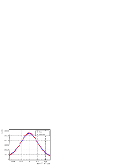
The difference in angle between the two reconstructed tracks provides a test of the ability of the simulation to reproduce multiple scattering through the target module. The distribution of the change in angle is presented for the silver target module in Fig. 5. The central width and most probable value (MPV) of this distribution are obtained from a fit to a Gaussian function. To minimize the effects of non-Gaussian tails to this value, the fit region is restricted to about its central value. The agreement in both width and MPV is shown in Table 4.
| Silver | Aluminium | |||||||
| Peak keV/ | Width keV/ | Peak mrad | Width mrad | Peak keV/ | Width keV/ | Peak mrad | Width mrad | |
| Data | 40.37 0.46 | 55.46 0.20 | -0.00 0.14 | 21.09 0.08 | 32.25 0.42 | 53.28 0.26 | 0.13 0.15 | 11.43 0.06 |
| Simulation | 43.36 0.43 | 54.84 0.26 | -0.20 0.11 | 20.65 0.10 | 32.98 0.57 | 52.21 0.25 | -0.09 0.12 | 11.30 0.05 |
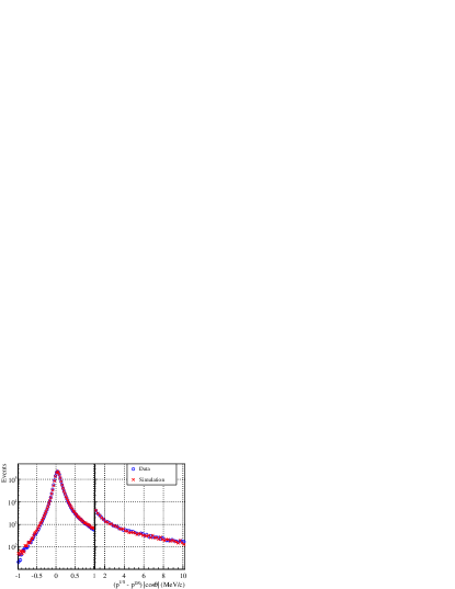
The second measurement comes from the change in momentum, which tests the validity of the simulation’s positron momentum loss. The measured momentum difference shows a dependence due to the planar geometry of the detector. The momentum loss is therefore studied using the quantity as shown for the silver target module in Fig. 6. Again a truncated Gaussian fit is used to determine the MPV and width of the central peak, which measures soft momentum loss processes. For Al there is agreement at the 1 keV/ level. For Ag there is a 3 keV/ difference in the MPV momentum loss, which is within the uncertainty of 3.5 keV/ for the simulated positron momentum loss Berger . The high momentum loss tail extending 10 MeV/ above the peak and 3 orders of magnitude below the peak height is due primarily to bremsstrahlung processes. The integrated counts in this tail validate the bremsstrahlung rate at the 1% level, in agreement with a separate evaluation based on broken tracks (Sec. V.2).
IV.2 Reconstruction Inefficiencies
The analysis of the far upstream stops data also determines the probability of not finding a track in one-half of the detector when it is successfully reconstructed in the other half. This inefficiency includes the possibility that the tracks physically scatter into or out of the fiducial region but it is dominated by the possibility of not reconstructing an existing track. The double difference between upstream and downstream halves of the detector and between data and simulation would affect the muon decay parameters, in particular.
A weighted average of the track inefficiency was compiled from the events that fall within the fiducial region for both data and the simulation for each target module (Table 5). The weighting was defined using the Bayesian interval for the ratio of the failed tracks over the total tracks for a given bin. Beam positron tracks are localized at the fiducial boundary and are therefore rather sensitive to inscattering and outscattering; for this reason they were removed from the calculation. Table 5 shows a clear difference in the upstream and downstream inefficiencies due to positron interactions in the target, but is reproduced by the simulation at the level. Positron interactions in the target module or first downstream chambers, including annihilation-in-flight, large angle scattering, or production of secondaries that confound the reconstruction, will produce such a difference in our inefficiency measurements.
| Target | Detector | Inefficiency () | ||
|---|---|---|---|---|
| half | Simulation | Data | Difference | |
| Al | US | 3.96 0.16 | 3.74 0.16 | 0.36 0.23 |
| DS | 5.71 0.18 | 6.15 0.19 | -0.30 0.28 | |
| Ag | US | 4.54 0.16 | 3.74 0.11 | -0.30 0.20 |
| DS | 7.13 0.18 | 7.47 0.15 | -0.58 0.25 | |
IV.3 Time Spectrum Fits
To check the consistency of data and simulation, of time calibration, and the absence of time-independent backgrounds in the data, fits of the selected events to the time dependence were performed for a typical data set and also for a simulation set. The fits included an overall normalization, the degree of initial muon polarization, and also a small time-dependent relaxation of the asymmetry Jamespmuxi . The fit range was from 2 s to 9 s following muon arrival to avoid a small decay time distribution bias below 1 from the algorithm that rejected beam positron pileup. Assuming zero uniform background and the accepted value of the muon lifetime, acceptable fit qualities were obtained for events in the decay parameter fit region. The confidence levels are 75% for set 84 and 6% for the corresponding simulation, using only statistical uncertainties. These results confirm that the tracks selected by the fiducial region in data are consistent with a pure sample of positrons from muon decays. However, no systematic evaluation of the lifetime measurement was attempted, as it was beyond the scope of our physics goals and not intrinsically relevant to the measurement of decay parameters.
V Blind analysis uncertainties and corrections
Most of the systematic uncertainties originate from a mismatch in the apparatus or in physics processes between the simulation and the experiment. These uncertainties are evaluated by purposely exaggerating the mismatch in a simulation and measuring the change in decay parameters between this modified simulation and a nominal simulation. The difference is the sensitivity of the decay parameter to this mismatch. The exaggeration produces statistically well determined sensitivities. A factor corresponding to the ratio between the exaggerated mismatch and the estimation of the real mismatch is used to rescale the sensitivity to obtain the systematic uncertainty. The sensitivity to a component of the analysis can be obtained by comparing via a decay parameter fit the spectra from a standard analysis and from an analysis with that component exaggerated, using the same data for both analyses. This approach, when possible, reduces the statistical uncertainties from the sensitivity evaluation. It relies on the assumption of linearity of the systematic uncertainties evaluated, which was verified to be valid for large uncertainties such as the bremsstrahlung production rate (Sec. V.2). Special attention was also given to avoid the double counting of a systematic uncertainty as in the case of the momentum resolution during the evaluation of the DC STRs (Sec. V.4). Table 6 summarizes the systematic uncertainties by categories that typically contain multiple independent uncertainties.
The weighted statistical uncertainties in Table 6 are computed from the statistical errors for the two targets, weighted according to the target dependent systematic errors. The weighted systematic uncertainties are the quadrature sum of the target independent systematic uncertainties and the appropriately weighted target dependent systematic uncertainties.
As described above, we calculate the systematic uncertainties for and due to a mismatch as and , where is our estimate of the possible size of the mismatch. is common to the and systematics, so represents a contribution to the correlation between and . The correlation for the Ag (Al) target measurement is given by the sum of the Ag (Al) and target independent correlations normalized by the quadratic sum of the Ag (Al) and target independent systematic uncertainties. The final total correlation is the sum of the Ag and Al target correlations weighted by the statistical weights used to determine the final decay parameter measurement.
| Category | Uncertainty () | |
|---|---|---|
| Target independent | ||
| Radiative corrections and | 1.3 | 0.6 |
| Momentum calibration | 1.2 | 1.2 |
| Chamber response | 1.0 | 1.8 |
| Resolution | 0.6 | 0.7 |
| Positron interactions111excluding bremsstrahlung | 0.5 | 0.1 |
| Others | 0.3 | 0.4 |
| Ag target | ||
| Bremsstrahlung rate | 1.8 | 1.6 |
| Stopping position | 2.0 | 6.0 |
| Target thickness | 3.2 | 2.2 |
| Statistical | 1.2 | 2.1 |
| Al target | ||
| Bremsstrahlung rate | 0.7 | 0.7 |
| Stopping position | 0.2 | 0.8 |
| Statistical | 1.3 | 2.4 |
| Weighted systematic uncertainty | 2.3 | 2.7 |
| Weighted statistical uncertainty | 1.2 | 2.1 |
| Total uncertainty | 2.6 | 3.4 |
V.1 Target independent uncertainties
Two systematic uncertainties are external to the TWIST measurement. The uncertainty on the radiative corrections is given by the effect of the missing leading term on the decay parameters Anastasiou . A numerical integration of this term in the TWIST fiducial regions showed that it has a similar shape, 5 times smaller than the term. The spectrum shape of the term is used to evaluate the change in decay parameters which gave a systematic uncertainty of () for (). The second external uncertainty is due to the significant correlation factor of 0.94 between the and the parameters. The impact of this correlation on the decay parameters is evaluated by performing the decay spectra fit with fixed at the world average value lowered or raised by 1 standard deviation. The changes in decay parameters are used as systematic uncertainties and are equal to () for ().
The chamber response category contains the systematic uncertainties for the STRs and the cathode foil position presented below, and also the asymmetry between upstream and downstream efficiency, the crosstalk, and the wire time offsets. The upstream-downstream asymmetry uncertainty is measured by scaling the upstream half of the - spectrum with respect to the downstream half according to the difference in inefficiencies between data and simulation extracted from the far upstream stops data (Sec. IV.2). The corresponding systematic uncertainty for () is (). All crosstalk in the electronics of nearby wires in the drift chambers should be removed by the analysis software. An upper limit on a potential systematic uncertainty due to remaining crosstalk is obtained by disabling the crosstalk removal and using the full change of () for () as the uncertainty. The wire time offsets are measured using different scintillators for the upstream and downstream halves of the detector which can lead to an asymmetry. The potential difference in this asymmetry between data and simulation (which was also calibrated) is responsible for a systematic uncertainty of () for ().
The spectrometer’s reconstruction resolution in angle and momentum is obtained from the far upstream stops data (Sec. IV). The - spectrum is smeared on an event-by-event basis to exaggerate the effect of a resolution mismatch. The rescaled sensitivity provides a systematic uncertainty for the momentum resolution of () for (). The angle resolution mismatch leads to a systematic uncertainty for both parameters.
The positron interaction category (Table 6) includes the systematic uncertainty for the backscattering of decay positrons from outside material that adds confusion to the track reconstruction. The rate of backscattering positrons normalized to the muons stopping in the target is used to measure the mismatch in outside material between data and simulation. The systematic effect of the outside material is determined by comparing a nominal simulation and the simulation matching set 83 in which the downstream beam package is added (Table 2). The corresponding systematic uncertainty for () is (). The decay parameter difference between sets 83 and 84, respectively with and without downstream beam package, is consistent with this uncertainty.
The category of systematic uncertainties under the name “others” in Table 6 contains uncertainties that are for both and . The overall spacing in of the wire chamber planes was established to a fractional accuracy of . An analysis with the positions exaggerated by a fractional change of showed a corresponding change in the momentum calibration. The changes in and were negligible. A small correction to the magnetic field is obtained by fitting an analytic function to the difference between the measured field map and the Opera-3D map. A comparison of set 84 analyzed with this correction with the nominal analysis is used to obtain corrections and associated uncertainties. This analysis shows significant corrections to the energy calibration parameters. However, after the new calibration is applied, the change to and is . Finally, the uncertainties for the muon and positron beam intensities are also part of this category and are negligible.
V.2 Bremsstrahlung and -electron production rate
A difference between data and simulation in the rates for the emission of bremsstrahlung photons or electrons would affect the decay parameter measurement. Primarily these processes modify the positron momentum and angle between the muon decay vertex and the beginning of the tracking region, thus altering the reconstructed - spectrum shape. Additionally a large change in positron momentum within the tracking region can lead to the identification of two separate track segments by the reconstruction algorithm. This second effect reduces the reconstruction resolution by shortening the primary decay positron track, but it can also be used to compare the bremsstrahlung and -electron production rates for data and simulation.
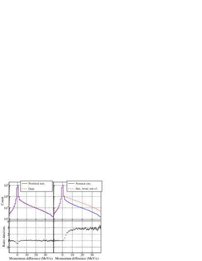
The bremsstrahlung production rate is evaluated by counting the number of events containing two reconstructed tracks from a single decay positron. The data and simulation counts are normalized to the number of muons stopping in the target. The momentum of the bremsstrahlung photon is deduced from the momentum difference between the two tracks and is shown in the left panel of Fig. 7. The agreement between data and simulation is excellent except near . The discrepancy there could be due to the loss of hits from corners of the drift cells, which happens more in data than in the simulation. These additional hits lead to a higher rate of broken tracks with very little momentum difference between the two track segments in the simulation. Events with a between 15 and 35 MeV/ are used for the comparison. The average ratio of the bremsstrahlung production rates from all the data sets to their corresponding simulations is equal to . Although this ratio is measured for the relatively low Z materials of the chambers, it is assumed to be applicable for the full range of materials in the detector. This assumption is supported by the target energy loss measurements (Sec. IV). The bremsstrahlung rate is strongly dependent on the target material. Thus the sensitivities to the production rate are measured separately for each target, from the difference in decay parameters between a nominal simulation and a simulation with the bremsstrahlung production rate exaggerated by a factor of 3. See the right panel of Fig. 7. The systematic uncertainties (Table 6) are given by the sensitivities rescaled by the factor . A simulation with a smaller exaggeration factor of 2 was also generated and analyzed, and its results confirm the assumption of linearity of the systematic uncertainty.
Evaluation of the electron production rate uncertainty is done similarly to that of the bremsstrahlung. The production rate is measured by requiring a third track from a negatively charged particle along with the two track segments from the decay positron. The momentum of the electron is measured directly from the reconstruction of the negatively charged track and used to select events with electrons in the momentum range () MeV/. The average ratio from all the data sets and their corresponding simulations is equal to . The sensitivities to the electron production rate are also evaluated using a simulation with a threefold exaggerated rate. The contribution is () for () to the Table 6 positron interaction uncertainties.
V.3 Momentum calibration
V.3.1 End points fits
The momentum mismatch between data and simulation at the end point, which is assumed to be linear with respect to based on geometrical considerations, is characterized by the parameters , and as shown in Eq. (10). However, if one assumes that the uncertainties are purely statistical, the linear fits result in a total of 212.9 for 168 degrees of freedom, corresponding to a value from all the data sets equal to 0.011. Evidently the behavior of the mismatch is not linear, possibly due to higher order effects or perhaps some underlying fine structure in the momentum spectrum for each angle bin. The manifest nonlinearity stems from the upstream end-point portions of the fits, while the downstream portions have larger statistical uncertainties that could mask any nonlinear behavior.
To account for this nonlinearity we add in quadrature an uncertainty of 1.6 keV/ to the statistical uncertainty of the momentum mismatch at each bin, in order to achieve an upstream reduced of one. When propagated to the uncertainties of the decay parameters, this results in systematic uncertainties of () in ().
The observed offset at the end-point between data and simulation is 10 keV/. To understand this difference quantitatively, a number of sources of systematic corrections and uncertainties must be considered. Approximately 4 keV/ of this total is due to a slightly incorrect scale used for the magnetic field in the simulation. Small corrections to the momentum calibration parameters were calculated from the best values for the target thicknesses, magnetic field map, and match of the muon stopping distribution (to be described in Sec. VI.1). Systematic uncertainties for these parameters have been determined using the same simulation studies that were used to determine the muon decay parameter uncertainties. The most significant items are from the magnetic field map, the STRs, the spacing of the chambers, the match of the muon stopping distribution, and the target thicknesses. Additionally, there is an uncertainty from soft momentum loss in the simulation, consisting of an ionization momentum loss uncertainty of 2% and a radiative momentum loss uncertainty of 3% Berger for the drift chamber and target materials used. After corrections, the magnitude of the mean slope parameters for each target is less than 5 keV/, and the mean offset magnitude is less than 7 keV/, both with systematic errors of 5 keV/. This level of agreement shows acceptable consistency of the data with the expected accuracy of the simulation.
V.3.2 Propagation model
The momentum mismatch between data and simulation is measured only at the kinematic end-point but is corrected over the entire spectrum. The predicted momentum dependence of this calibration depends on the source of the momentum mismatch between data and simulation. For instance, a difference in solenoid magnetic field strength leads to a momentum mismatch that depends linearly on the momentum and is referred to as a scale. Another example is a mismatch in target thickness, which translates into an angle-dependent shift of the momentum (to first order), with the angle dependence measured by the slopes and . Most of the observed offset at the end-point could not be attributed to a unique source. Therefore it was assumed that the propagation of the momentum mismatch is a mixture of shift and scale.
For this reason the decay parameters were computed for the two extreme cases of propagation which correspond to a pure shift with the form
| (12) |
or a pure scale, given by
| (13) |
where and were defined in the context of Eq. 4. The average values of the and parameters using the shift and the scale propagations are different respectively by and . Their mean is used for the decay parameter. Half of the difference between shift and scale is used as the uncertainty to cover the two extreme possibilities. Therefore the systematic uncertainty from the propagation model is () for ().
V.4 DC STRs
The accuracy of the helix reconstruction depends on the quality of the STRs. In particular, differences between the respective accuracies of data and simulation STRs can lead to a bias in the decay parameter measurement. The STRs were derived in both cases using the two-dimensional time residual distributions covering the entire drift cell () from the helix fitter. The sensitivity to a mismatch in STRs is measured by creating simulation STRs containing the difference between data and simulation STRs. First 44 are created by taking the difference between the data and the simulation for each DC. The 44 are fitted with a fifth order polynomial function to guarantee the smoothness of the STRs created in the next step. Second 44 STR tables are created by adding the 44 polynomial functions exaggerated by a factor of ten to 44 duplicates of the simulation STRs. A simulation is reanalyzed with these new STRs and this set is fitted against the unmodified set to measure a change in decay parameters. The corresponding sensitivity of the decay parameters to the STRs changes significantly if the propagation model for the momentum calibration is a shift or a scale. For this reason the sensitivities from both models are averaged and the total sensitivity is () for () to STRs exaggerated by a factor of 10.
The momentum resolution at the kinematic end-point is very different between the standard and these exaggerated-STR analyses of the simulation. However the impact of the resolution on the decay parameters is already taken into account in a separate systematic uncertainty. The systematic effect from the resolution must be subtracted from the STR sensitivities evaluated in this section to avoid double counting.
The sensitivities to the reconstruction resolution are evaluated from the differences in decay parameters between a nominal spectrum and spectra created with the events smeared in momentum by different values. This procedure is equivalent to a degradation in resolution. The contributions of the resolution to the STR sensitivities, which must be subtracted from the total sensitivities, are and for and . Finally each sensitivity is scaled down by the exaggeration factor of 10 to give the systematic uncertainty for the DC STRs of () for ().
V.5 Cathode foil position
The relative position of each cathode foil with respect to adjacent anode wires has two effects on the detector response. First of all it modifies the electric field and consequently the STRs. This effect is included in the plane dependent measurement of the STRs in data and therefore does not lead to any additional systematic uncertainty. The second effect is the change of the drift cell size which can change the number of cells crossed by each positron. This has an impact on the track reconstruction, in particular on the resolution of the left-right ambiguity in the helix fitter.
In the apparatus there are two different sources of uncertainty on the foil position. The first uncertainty is due to the DC outer foil bulging toward or away from the wires as a result of the differential pressure between the DCs and the helium-nitrogen gas mixture surrounding the chambers. The permanent foil bulge was toward the wires (6022) m (average) during the 2006 run period, and away from the wires (822) m during 2007. The second source of uncertainty comes from the construction of the chambers and was estimated to be 100 m on average.
The sensitivity of the decay parameters to the cathode foil position is evaluated by generating a simulation with cathode foils moved toward the wires by 500 m, without modifying the STRs. The fit of this exaggerated simulation against the corresponding nominal simulation gives a sensitivity of and for and . In this modified simulation the drift cell size is reduced for all the planes but in reality some drift cells are potentially larger in data than they are in simulation. Therefore the average systematic effect is smaller than the estimated sensitivity. For this reason the cathode foil position uncertainties from the bulge and the chamber construction are not added in quadrature but instead only the largest uncertainty of 100 m is considered, leading to an exaggeration factor of 5. The corresponding rescaled systematic uncertainty is () for ().
V.6 Statistics bias correction
A sensitivity to the difference in statistics between data and simulation was discovered in the minimization technique used by the decay parameter fit and the momentum calibration. In the situation where the data and simulation spectra have the same number of events, the difference of the two asymmetric Poisson distributions of two bins leads to a symmetric probability distribution for the residuals. However all the simulations contain 2 to 3 times more events than their corresponding data set to reduce the statistical uncertainty for the decay parameters. This creates an asymmetric distribution for the residuals and a bias in the minimization Barlow .
The biases of the decay parameter fit and the momentum calibration fit were evaluated by performing the fits between a data set and subsets of the simulation with matching statistics. For each fit parameter, the difference between the average of the subsets and the results using the whole simulation corresponds to the bias. Corrections of and for and were applied to account for the average fitting bias of the decay parameters. The momentum calibration fitting bias corrections were applied differently, on a set by set basis, and on the decay parameter measurements from the shift and the scale propagation of the calibration to the spectrum. The values of the corrections range between and ( and ) for ().
VI Postblind analysis
The hidden parameters of the blind analysis were revealed once the differences of the three decay parameters between data and simulation were confirmed and the systematic uncertainties were fully evaluated. The results for the three parameters were consistent with the SM. However, the product was . Although the sign of the deviations of the individual decay parameters from the SM is not constrained in the generalized matrix element treatment Fetscher:1986 , the product must be . This product can be identified with the asymmetry between the extremes of and evaluated at by using Eqs. (4), (5), and (6).
A measurement of could have been due to the matrix element treatment or the momentum-angle functional form being inadequate to describe the data, but it could also have been due to a systematic uncertainty or correction missing or not evaluated properly in the analysis. Furthermore, from the blind analysis was different for the Ag and Al target data by 3.8 . Both the large value of and the mismatch between Ag and Al target data triggered an exhaustive review of the blind analysis and special scrutiny of various systematic effects that could explain these results. Among the tests performed, effects such as decays (where is a long-lived unobserved particle), an incorrect value of the parameter, or plausible errors in the radiative correction implementation, did not resolve the mismatch. However we found two corrections that were missed during the blind analysis.
VI.1 Additional systematic uncertainties and corrections
The effect of the muon radiative decay on the - spectrum is included in the radiative corrections of the decay positron spectrum of the simulation (Sec. III.1). However we neglected to simulate the photon from radiative decays. Although the wire chambers are insensitive to photons, the electrons and positrons from pair production or Compton scattering of the photons can affect the track reconstruction. These processes occur at different rates in Ag and Al and therefore potentially bias the Ag and Al measurements differently. The effect on the decay parameters is measured using two simulations of pure muon radiative decay using the Fronsdal and Überall formula fron59 to calculate the momentum and angle of the decay positrons and the photons. One simulation contains all the standard physics processes while the second simulation does not include the pair production and the Compton scattering of the photon so that, as in the nominal simulation, the radiative decay photons are absent. The decay parameter difference is renormalized using the branching ratio of % from PDG . The corrections to and for the Ag data are and , and they are negligible for the Al data.
The second category of corrections and related refinement of systematic uncertainties is due to the large sensitivity to energy loss through bremsstrahlung emission by the positron as it travels through the target. We expected the momentum calibration to correct for a mean muon stopping position difference (MSPD) between data and simulation. A match with precision at the level of 1 m is required, but the kinematic edge was not very sensitive to the large changes in momentum due to bremsstrahlung that can affect the spectrum in the fiducial region. Also, we assumed that corresponded to MSPD , which turned out not to be true. An improved technique was developed to determine MSPD. For the blind analysis the systematic uncertainty for a mismatch in bremsstrahlung production rate was evaluated only for the Ag target and applied to all the data. In the postblind procedure, it is evaluated for each target, and a separate uncertainty is added for a mismatch in target thickness.
A measurement based on the distribution of the last wire plane hit by the muons is used to evaluate the muon’s MSPD between data and simulation. The last wire plane distributions are normalized to the number of muons stopping in the target defined by the counts in PC 6 (wire plane 28) which is located just upstream of the target (Fig. 8).
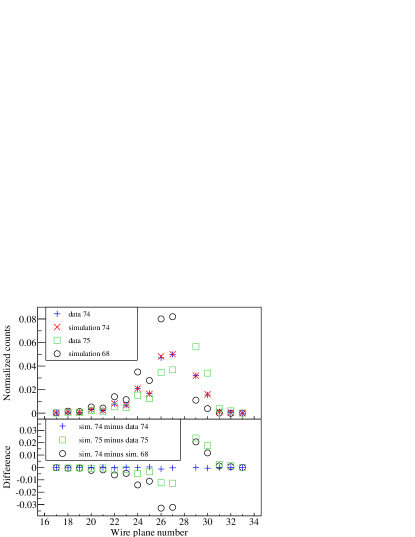
The differences between data and simulation last wire plane distributions show agreement at the percent level for all planes for data sets 68, 74 and 76, which confirms a match in the mean and the widths of the stopping distributions. However, disagreements for other sets identified a sensitivity to MSPD. Different methods were tested to establish MSPD with improved precision. It was found that MSPD could be measured using an average of the PC 5 and PC 7 fractional differences (wire planes 27 and 29) where the sensitivity is the highest. We verified that MSPD measurements from other planes are consistent with the measurement from PC 5 and PC 7. The relationship between the average fractional difference and the MSPD is extracted from the comparison of simulations with known non-zero MSPDs such as between the simulations of the data sets 68 and 74 shown Fig. 8. Each data set and its corresponding simulation were compared and MSPDs of up to 1.6 m were determined for the Ag target and 3.8 m for the Al target. The sensitivity of the decay parameters to MSPD is determined by creating - spectra for different depth intervals in the target using the true stopping position of the muons in the simulation. Set by set corrections are applied and range from 0.0 to (0.0 to ) for (). Although MSPD is larger in Al, the largest corrections are for the Ag target (set 75) because of a higher density and bremsstrahlung production rate in Ag. We estimate the MSPD uncertainty to be 1 m for Ag and 2 m for Al. The systematic uncertainties on the correction, determined from the sensitivity to MSPD, are respectively for the Ag and Al targets () and () for () (under “stopping position” in Table 6).
The accurate measurement of target thickness is based on a destructive test that could only be performed after the experiment. It gives a thickness of m and m for the Ag and Al targets respectively. The simulation used the prior estimate of the Ag (Al) target thickness of 29.5 m (71.0 m), which was based on measurements of material samples that were similar to the targets, but obviously not identical. The impact on the decay parameters of the mismatch in Ag target thickness was determined by generating a simulation with a 65 m thick target. The corresponding systematic uncertainty for () is (). On the other hand, the systematic uncertainties for the mismatch in Al target thickness were negligible with values .
VI.2 Results
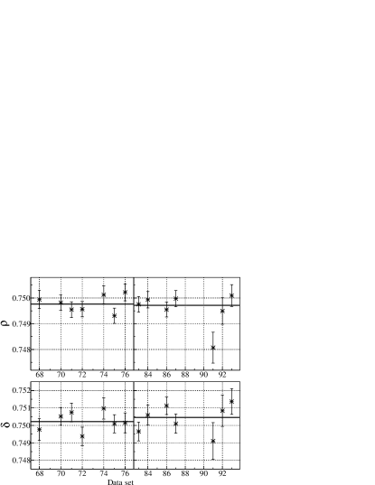
The final results are extracted from all data sets identified as valid for analysis of and . These sets are unchanged from the blind analysis. However, the postblind result for includes correlation information from the measurement of in five data sets not used for , which reduces its statistical uncertainty but does not change the central value. This analysis has already been published separately Jamespmuxi . The consistency is shown in Fig. 9 for measurements taken under various experimental conditions (Tables 1 and 2), demonstrating that the simulation reproduces these conditions accurately. The Ag and Al data are fitted separately and then are combined using the target dependent systematic uncertainties.
The additional corrections and systematic uncertainties determined during the reevaluation of the analysis (Sec. VI.1) change the central values of and by and ; both changes are less than the total assessed systematic uncertainties, which themselves changed by less than . The modified values of for Ag and Al data are now consistent within , while has decreased but remains somewhat greater than unity. The final TWIST results for and are
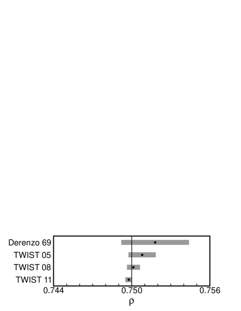
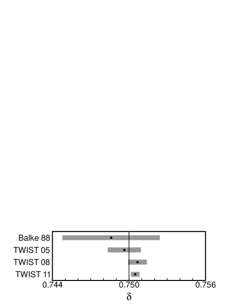
These results represent an improvement of a factor of respectively 14 and 11 over the pre-TWIST direct measurements. They are consistent with the SM predictions of and furthermore agree with previous measurements (Fig. 10).
VII Theoretical implications
VII.1 Global Analysis of Muon Decay
A new global analysis of all available muon decay data has been performed including the final TWIST results for the decay parameters and their correlations Jamespmuxi . All other input values are the same as in the analysis of gagliardi:2005 . The global analysis used a Monte Carlo method similar to that of burkard:1985 to map out the joint probability distributions for 10 variables (see Table 7), each of which is a bilinear combination of the weak coupling constants . The constraint of is applied (see Eq. (2)), resulting in 9 independent variables; the best fit values and 90% confidence limits are given in Table 7. The decay parameters could then be written in terms of these independent variables, and the results are included in Table 7. The present analysis makes significant improvements in the limits on , , and compared to the 2005 analysis, and tightens several of the other limits.
| Parameter | Global analysis results () |
| Parameter | Global analysis results |
The results from this global analysis can be used in Eq. (2) to place limits on the magnitudes of the weak coupling constants ; the exceptions are and , which are determined more sensitively from inverse muon decay, . These limits are presented in Table 8. Tighter limits from the present analysis of up to a factor of 2 compared to the 2005 analysis are found in and .
A new indirect limit on the value of can be obtained from the global analysis. The linear combination
| (14) |
combined with the constraints , , and , builds in the physical condition , which is required to avoid a negative muon decay probability near the end point [see Eq. (4)]. We find or (90% C.L.). This is a significant improvement over the previous limit of Jodidio .
The quantity represents the total probability for a right-handed muon to decay into any type of electron, a process forbidden under the SM weak interaction. The new limits on and shown in Table 7 yield a new 90% confidence limit upper bound on the combined probability , a factor of 6 improvement over the limit from the pre-TWIST numbers.
VII.2 Neutrino mixing
It is now established that flavor mixing occurs in the neutrino states SuperK ; SNO . Thus the neutrino state summations in Eq. (4) need to extend over the additional kinematically allowed states and mixings since the matrix elements of Eq. (1) are evaluated in the flavor basis. Doi et al. Doi have calculated the dependence of the decay parameters on the neutrino masses and mixings when only chiral vector weak couplings are allowed. These calculations have shown that, when all of the neutrinos involved are much lighter than the muon mass, as is the case for , , and , the decay parameters in Eqs. (5) and (6) are unaffected. However if there are additional mixed neutrino states with large right-handed Majorana masses, the decay rate is modified. For seesaw model extensions of the SM, the effect on the muon decay parameters is below the precision of the present measurement.
VII.3 Nonlocal tensor interaction
The coupling constants and are set to zero in the general 4-fermion interaction [Eq. (1)] because their corresponding matrix elements cancel out. However by abandoning locality Chizhov94 ; Chizhov_Review , one can redefine the tensor interaction as
| (15) |
where is the momentum transfer of some virtual boson. This form of the tensor interaction permits nonzero contributions from and , in addition to and . If the tensor interaction couples equally to quarks and leptons, pion decay data require , , and to be very small Voloshin ; Chizhov_Review . The seesaw mechanism to generate neutrino masses would require these same three coupling constants to be identically zero in muon decay. For these reasons, Chizhov Chizhov_Review explored how the muon decay spectrum would be changed if the standard model were augmented by the addition of a single additional coupling constant, .
Nonzero requires the introduction of a new muon decay parameter, , in the differential muon decay spectrum, such that Eqs. (5) and (6) become:
| (16) | |||||
| (17) | |||||
The term in Eq. (16) introduces a negligible distortion in the isotropic distribution relative to the precision of TWIST. In contrast, the linear term in Eq. (17) represents a significant modification to . Chizhov Chizhov_Review finds that it increases the integral forward-backward asymmetry by a factor .
The three decay parameters measured by TWIST also receive direct contributions from :
| (18) |
Thus, provides both linear and quadratic modifications to the muon decay spectrum. This combination implies the linear fitting procedure used in this analysis [Eq. (8)] cannot be altered to fit directly.
A study Williams was performed using the theoretical - spectrum to determine how a nonzero value of would distort the values we obtain for , , and . We find
| (19) |
The latter two equations imply
| (20) |
When Eqs. (19) and (20) are combined with our measured values for , , , and their correlations to calculate the probability distribution for , we find (90% C.L.).
VIII Summary
These new measurements of the muon decay spectrum culminate the TWIST experimental program and are about 1 order of magnitude more precise for each one of the three decay parameters than measurements prior to TWIST. In fact, it has been more than 40 years since the previous precision measurement of , and no experimental effort in the intervening years has succeeded in surpassing the precision quoted in Ref. Derenzo , until TWIST. For , the interval has been more than 20 years since the last measurement Balke . Our final results supersede our intermediate values. They are consistent with SM predictions, placing more stringent limits on physics beyond the SM in the weak interaction.
Acknowledgments
We thank all early TWIST collaborators and students for their substantial contributions. We also thank C. Ballard, M. Goyette, S. Chan, A. Rose, P. Winslow, and the TRIUMF cyclotron operations, beamlines, and support personnel. Computing resources were provided by WestGrid and Compute/Calcul Canada. This work was supported in part by the Natural Sciences and Engineering Research Council and the National Research Council of Canada, the Russian Ministry of Science, and the U.S. Department of Energy.
References
- (1) W. Fetscher, H.-J. Gerber, and K.F. Johnson, Phys. Lett. B173, 102 (1986).
- (2) W. Fetscher and H.J. Gerber, in Review of Particle Physics, K. Nakamura et al. (Particle Data Group), J. Phys. G 37, 075021 (2010), p. 521.
- (3) L. Michel, Proc. Phys. Soc. A63, 514 (1950); C. Bouchiat and L. Michel, Phys. Rev. 106, 170 (1957); T. Kinoshita and A. Sirlin, Phys. Rev. 107, 593 (1957); T. Kinoshita and A. Sirlin, Phys. Rev. 108, 844 (1957).
- (4) M. V. Chizhov, Mod. Phys. Lett. A8, 2753 (1993).
- (5) M. V. Chizhov, Physics of Particles and Nuclei 42, 93 (2011).
- (6) J.R. Musser et al. (TWIST Collaboration), Phys. Rev. Lett. 94, 101805 (2005).
- (7) A. Gaponenko et al. (TWIST Collaboration), Phys. Rev. D 71, 071101(R) (2005).
- (8) R.P. MacDonald et al. (TWIST Collaboration), Phys. Rev. D 78, 032010 (2008).
- (9) R. Bayes et al. (TWIST Collaboration), Phys. Rev. Lett. 106, 041804 (2011).
- (10) J.F. Bueno et al. (TWIST Collaboration), Phys. Rev. D 84, 032005 (2011); 85, 039908(E) (2012).
- (11) C.A. Gagliardi, R.E. Tribble, and N.J. Williams, Phys. Rev. D 72, 073002 (2005).
- (12) R.S. Henderson et al., Nucl. Instrum. Methods A 548, 306 (2005).
- (13) Y. Davydov et al., Nucl. Instrum. Methods A 461, 68 (2001).
- (14) J.F. Bueno et al., Phys. Rev. B 83, 205121 (2011).
- (15) Opera 3D Simulation Software, Vector Fields.
- (16) J. Hu et al., Nucl. Instrum. Methods A 566, 563 (2006).
- (17) A. Gaponenko, arXiv:1104.2914 [hep-ex].
- (18) geant Detector Description and Simulation Tool, CERN Application Software Group, Geneva, Switzerland, 1994, Version 3.21.
- (19) R. Veenhof, Garfield: Simulation of gaseous detectors, CERN program Library long writeup W5050 (2003) (unpublished).
- (20) A. B. Arbuzov, Phys. Lett. B524, 99 (2002); A. Arbuzov, A. Czarnecki, and A. Gaponenko, Phys. Rev. D 65, 113006 (2002); A. Arbuzov and K. Melnikov, Phys. Rev. D 66, 093003 (2002); A. Arbuzov, J. High Energy Phys. 2003, 063 (2003).
- Davydychev et al. (2001) A. Davydychev, K. Schilcher, and H. Spiesberger, Eur. Phys. J. C 19, 99 (2001).
- (22) F. James, Nucl. Instrum. and Methods in Phys. Research 211, 145 (1983).
- (23) G. Lutz, Nucl. Instrum. and Methods A 273, 349 (1988).
- (24) H. Bichsel, D.E. Groom, and S.R. Klein, in Review of Particle Physics, K. Nakamura et al. (Particle Data Group), J. Phys. G 37, 075021 (2010), p. 285.
- (25) F. James, MINUIT: Function Minimization and Error Analysis, CERN Program Library Entry D 506 (1994).
- (26) A. Grossheim, J. Hu, and A. Olin, Nucl. Instrum. Methods A 623, 954 (2010).
- (27) M.J. Berger and S.M. Seltzer, National Academy of Sciences Report No. 39, 1964.
- (28) C. Anastasiou, K. Melnikov, and F. Petriello, J. High Energy Phys. 09, 14 (2007).
- (29) R. Barlow and C. Beeston, Computer Physics Communications 77, 219 (1993).
- (30) C. Fronsdal and H. Überall, Phys. Rev. 113, 654 (1959).
- (31) H. Burkard et al., Physics Letters B160, 343 (1985).
- (32) A. Jodidio et al., Phys. Rev. D 34, 1967 (1986); 37, 237(E) (1988).
- (33) Y. Fukuda et al., Phys. Rev. Lett. 81, 1562 (1998).
- (34) Q. R. Ahmad et al., Phys. Rev. Lett. 89, 011301 (2002).
- (35) M. Doi, T. Kotani, and H. Nishiura, Prog. Theor. Phys. 118, 1069 (2007); 122, 805(E) (2009).
- (36) M. B. Voloshin, Phys. Lett. B. 283, 120 (1992).
- (37) K.S. Williams, private communication (2006).
- (38) S.E. Derenzo, Phys. Rev. 181, 1854 (1969).
- (39) B. Balke et al., Phys. Rev. D 37, 587 (1988).