Abstract

We investigate both analytically and numerically the renormalization group equations in $2D$ $Z(N)$ vector models. The position of the critical points of the two phase transitions for $N>4$ is established and the critical index $\nu$ is computed. For $N$=7, 17 the critical points are located by Monte Carlo simulations and some of the corresponding critical indices are determined. The behavior of the helicity modulus is studied for $N$=5, 7, 17. Using these and other available Monte Carlo data we discuss the scaling of the critical points with $N$ and some other open theoretical problems.

  e-mail addresses:

^†oleg@bitp.kiev.ua,   ^∗vchelnokov@i.ua,   ^¶cortese, fiore, papa  @cs.infn.it,

^‡gravina@ucy.ac.cy

1 Introduction

The Berezinskii-Kosterlitz-Thouless (BKT) phase transition was originally discovered in the two-dimensional ($2D$) $XY$ model in the first half of the seventies [1, 2]. Since then it was realized that this type of phase transition takes place in a number of other models including discrete $2D$ $Z(N)$ models for large enough $N$ and even $3D$ gauge models at finite temperature (see [3, 4] for a recent study of the deconfinement transition in $3D$ $U(1)$ lattice gauge theory). Here we are interested in the phase structure of $2D$ $Z(N)$ vector models . On a $2D$ lattice $\Lambda=L^{2}$ with linear extension $L$ and periodic boundary conditions, the partition function of the model can be written as

$$Z(\Lambda,\beta)=\left[\prod_{x\in\Lambda}\frac{1}{N}\sum_{s(x)=0}^{N-1}\right]\ \exp\left[\sum_{x\in\Lambda}\ \sum_{n=1,2}\ \beta\ \cos\frac{2\pi}{N}(s(x)-s(x+e_{n}))\right]\ .$$ (1)

The BKT transition is of infinite order and is characterized by the essential singularity, i.e. the exponential divergence of the correlation length. The low-temperature or BKT phase is a massless phase with a power-law decay of the two-point correlation function governed by a critical index $\eta$. The $Z(N)$ spin model in the Villain formulation has been studied analytically in Refs. [6, 7]. It was shown that the model has at least two BKT-like phase transitions when $N\geq 5$. The critical index $\eta$ has been estimated both from the renormalization group (RG) approach of the Kosterlitz-Thouless type and from the weak-coupling series for the susceptibility. It turns out that $\eta(\beta^{(1)}_{\rm c})=1/4$ at the transition point from the strong coupling (high-temperature) phase to the massless phase, i.e. the behavior is similar to that of the $XY$ model. At the transition point $\beta^{(2)}_{\rm c}$ from the massless phase to the ordered low-temperature phase, one has $\eta(\beta^{(2)}_{\rm c})=4/N^{2}$. A rigorous proof that the BKT phase transition does take place, and so that the massless phase exists, has been constructed in Ref. [8] for both Villain and standard formulations. Monte Carlo simulations of the standard version with $N$=6, 8, 12 were performed in Ref. [9]. Results for the critical index $\eta$ agree well with the analytical predictions obtained from the Villain formulation of the model. In Refs. [10, 11] we have started a detailed numerical investigation of the BKT transition in $2D$ $Z(N)$ models for $N=5$, which is the lowest number where this transition can occur. Our findings support the scenario of two BKT transitions with conventional critical indices.

Despite of this progress, some theoretical issues remain unresolved.

• Status of the critical index $\nu$. This index governs the behavior of the correlation length $\xi$, namely it is expected that in the vicinity of the phase transition one has $\log\xi\sim a/(\beta_{c}-\beta)^{\nu}$. In all numerical studies one postulates the $XY$ value $\nu=1/2$. This value appears compatible with numerical data. However, no theoretical arguments exist which support this value. Moreover, the study of the Hamiltonian version of $Z(N)$ models via the strong coupling expansion combined with the Padé approximant points to a different value for $N$=5, 6. Only for $N=12$ one finds $\nu\approx 1/2$ [6].

• The scaling of critical points $\beta_{c}^{(1,2)}$ with $N$ is still unknown. What is seen from the available numerical data is that $\beta_{c}^{(1)}$ approaches the $XY$ critical point rather fast, probably exponentially with $N$, while $\beta_{c}^{(2)}$ scales like some power of $N$.

Most theoretical knowledge about the critical behavior of the $XY$ model comes from the solution of the RG equations [2]. Explicit solutions for the RG equations of the arbitrary $Z(N)$ model are unknown. Moreover, to the best of our knowledge, even approximate and/or numerical solutions have not been obtained.

One of the goals of the present paper is to fill this gap by constructing both numerical and approximate analytical solutions to the RG equations. Another goal is to continue the numerical study of $2D$ $Z(N)$ vector models and to compare results with analytical predictions.

The paper is organized as follows. In the next section we investigate the system of RG equations describing the critical behavior of $Z(N)$ models in the Villain formulation. This allows us to calculate the position of critical points for all $N$ and to compute the critical index $\nu$. In the section 3 we study numerically the models for $N$=7 and 17 . We locate the transition points and compute some critical indices. Then we present and discuss our results for the helicity modulus. Section 4 is devoted to the analysis of the dependence of the critical points on $N$ and the comparison with the RG prediction. Finally, we summarize our results in section 5.

2 Analysis of RG equations

The system of RG equations describing the critical behavior of $2D$ $Z(N)$ models is given by [6]

$$\frac{dx}{d\tau}\ =\ \frac{N^{2}}{4}\ z^{2}-x^{2}y^{2}\ \ ,\;\;\;\;\;\;\;\frac{dy}{d\tau}\ =\ (2-x)y\ \ ,\;\;\;\;\;\;\;\frac{dz}{d\tau}\ =\ \left(2-\frac{N^{2}}{4x}\right)z\ ,$$ (2)

where the parameters $x,y,z$ are initially defined as

$$x=\pi\beta\ ,\;\;\;\;\;\;\;y=2\pi\exp\left(-\frac{1}{2}\pi^{2}\beta\right)\ ,\;\;\;\;\;\;\;z=2\pi\exp\left(-\frac{N^{2}}{8\beta}\right)\ ,$$ (3)

and $a=\exp(\tau)$ is the lattice spacing .

This system of RG equations has been obtained for the Villain formulation of the model. All available numerical data show that the standard and the Villain formulations belong to the same universality class in the case of the $XY$ model. This probably holds also for $Z(N)$ models. The only case where universality has been questioned is $Z(5)$, where it was found numerically that the helicity modulus has a different behavior in the vicinity of $\beta_{c}^{(1)}$: while it jumps to zero crossing the critical point in the Villain formulation, it goes to zero smoothly in the standard formulation [12].

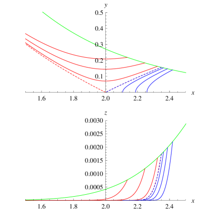
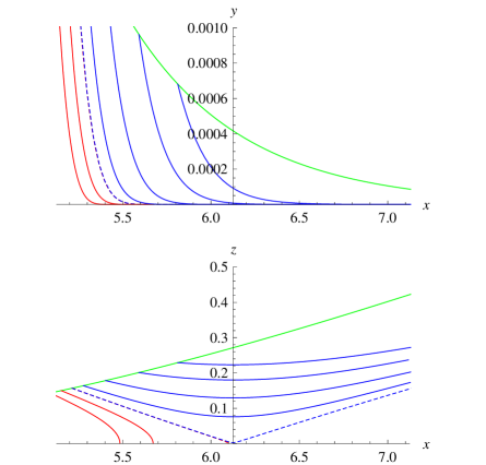
Figure 1: (Color online) Renormalization group trajectories for $N=7$ in the vicinity of the first phase transition (left) and in the vicinity of the second phase transition (right). The upper line shows initial values.

Table 1: Values of $\beta_{c}^{(1,2)}$ obtained from analytical and numerical solutions of Eqs. (2) for various values of $N$.

$N$	$\beta_{c\ \rm an}^{(1)}$	$\beta_{c\ \rm num}^{(1)}$	$\beta_{c\ \rm an}^{(2)}$	$\beta_{c\ \rm num}^{(2)}$
5	0.726050	0.741654	0.841969	0.853845
6	0.739670	0.747749	1.212435	1.219515
7	0.740256	0.747851	1.650259	1.659667
8	0.740266	0.747853	2.155441	2.167726
9	0.740266	0.747853	2.727980	2.743528
$\infty$	0.7403	0.7479	-	-

The system (2) has two sets of the fixed points. The first one

$$x=2\ ,\;\;\;\;\;y=0\ ,\;\;\;\;\;z=0\ ,$$ (4)

corresponds to a transition from the massive to the massless phase. The second one

$$x=\frac{N^{2}}{8}\ ,\;\;\;\;\;y=0\ ,\;\;\;\;\;z=0\ ,$$ (5)

describes the transition from the massless to the ordered phase. One can see that in the vicinity of the first fixed point the behavior of the solution in the $\tau\to\infty$ limit is the same as in the $XY$ model, i.e for $\beta\geqslant\beta_{c}^{(1)}$, $x$ tends to $x_{\infty}\geqslant 2$, $y$ tends to $0$, and for $\beta<\beta_{c}^{(1)}$, $y$ tends to infinity ($z$ tends to zero in both cases). Thus, $\beta_{c}^{(1)}$ may be determined as the value of $\beta$ at which the solution goes to the point $x=2,\ y=z=0$. Clearly, $\beta_{c}^{(2)}$ can be determined in a similar fashion, studying the system around the second fixed point $\beta=\frac{N^{2}}{8\pi}$ (the behavior of $y$ and $z$ is reversed). Then, one can easily compute the RG trajectories starting from the initial values (3). As an example, RG trajectories, projected onto $x$-$y$ and $x$-$z$ planes, are shown in Fig. 1 for $N=7$. Dashed lines show the trajectory at the critical point. Numerical values of critical points for various values of $N$ are given in Table 1.

To establish how the critical points scale with $N$ and to calculate the critical index $\nu$, it is desirable to have an analytical solution for the system (2). In the absence of the exact solution, we attempt here to construct an approximate solution, valid for large values of $N$. Making the following change of variables

$$x\ =\ 2+\frac{1}{2}\ \xi\ ,\;\;\;\;\;\;\;y\ =\ \sqrt{\frac{\omega}{8}}\ ,\;\;\;\;\;\;\;z\ =\ \exp\left[\left(2-\frac{N^{2}}{8}\right)\tau+\frac{N^{2}}{32}\ \eta\right]\;,$$ (6)

and then linearizing the system (2) around the first fixed point, one finds

$$\frac{d\xi}{d\tau}\ =\ -\omega+\frac{N^{2}}{2}\ \epsilon(\eta)\ \ ,\;\;\;\;\;\;\;\frac{d\omega}{d\tau}\ =\ -\xi\ \omega\ \ ,\;\;\;\;\;\;\;\frac{d\eta}{d\tau}\ =\ \xi\ .$$ (7)

Here

$$\epsilon(\eta)\ =\ \exp\left[\left(4-\frac{N^{2}}{4}\right)\tau+\frac{N^{2}}{16}\ \eta\right]\ =\ z^{2}$$ (8)

is treated as a small function for large $N$. This is valid in two cases: 1) $N\gg 4$ and 2) $\tau\to\infty$ if $N>4$.

To study the system around the second fixed point $x=\frac{N^{2}}{8}$, we make the following change of variables:

$$x\ =\ \frac{N^{2}}{8}\ (1-\xi/4)\ ,\;\;\;\;\;\;\;y\ =\ \exp\left[\left(2-\frac{N^{2}}{8}\right)\tau+\frac{N^{2}}{32}\ \eta\right]\ ,\;\;\;\;\;\;\;z\ =\ \sqrt{\frac{\omega}{8}}\ .$$ (9)

The linearization of the system (2) around the second fixed point leads to the same system of equations (7). This means that the solution of the system in terms of $\xi$, $\omega$ and $\epsilon$ will be the same as for the first critical point - we only have different initial conditions.

To the first order in $\epsilon(\eta)$, one obtains

$$x\ =\ 2+\frac{1}{2}\ (\xi_{0}+\xi_{1})\ ,\;\;\;\;\;\;\;\omega\ =\ -\frac{d\xi_{0}}{d\tau}-\frac{d\xi_{1}}{d\tau}+\frac{N^{2}}{2}\ \epsilon(\eta_{0})\ ,\;\;\;\;\;\;\;\eta_{0}\ =\ \int\xi_{0}d\tau\ +\ C_{3}\ .$$ (10)

Here $\xi_{0}$ is the solution of the system in the limit $N\to\infty$,

$$\frac{d\xi_{0}}{d\tau}+\frac{1}{2}\ \xi_{0}^{2}\ =\ C\ ,$$ (11)

$\xi_{1}$ describes the first nontrivial corrections and obeys the following linear equation:

$$\frac{d\xi_{1}}{d\tau}+\xi_{0}\xi_{1}\ =\ g(\tau)\ ,\;\;\;\;\;\;\;g(\tau)\ =\ \frac{N^{2}}{2}\ \epsilon(\eta_{0})+\frac{N^{2}}{2}\ \int\epsilon(\eta_{0})\ \xi_{0}\ d\tau\ .$$ (12)

The solution for $\xi_{0}$ reads

$$\xi_{0}\ =\ 2C_{1}\coth{C_{1}(\tau-\tau_{0})}\ ,\;\;\;\;\;\;\;C_{1}^{2}\ =\ \frac{1}{2}\ C\ ,$$ (13)

while the solution for $\xi_{1}$ vanishing for $N\to\infty$ can be presented as

$$\xi_{1}\ =\ \exp(-\eta_{0})\ \int g(\tau)\exp(\eta_{0})\ d\tau\ .$$ (14)

To find critical points, consider the zero-order approximation (13). In the limit $C\to 0$ (critical line of the model) and taking $C_{3}=-2\ln\sinh{C_{1}(C_{2}-\tau_{0})}$, the solution can be written as

$$\xi_{0}\ =\ \frac{2}{\tau-\tau_{0}}\ ,\;\;\;\;\;\;\;\omega_{0}\ =\ \frac{2}{\left(\tau-\tau_{0}\right)^{2}}\ ,\;\;\;\;\;\;\;\eta_{0}\ =\ 2\ln\frac{\tau-\tau_{0}}{C_{2}-\tau_{0}}\ .$$ (15)

We fix $\tau_{0}$ from the requirement that $\xi_{0}(0)$ and $\omega_{0}(0)$ satisfy the initial conditions for $x$ and $y$ given in (3) (this effectively means that $\xi_{0}$ and $\omega_{0}$ describe the critical trajectory of the $XY$ model). Hence,

$$2\pi\exp{\left(-\frac{1}{2}\pi\left(2-\frac{1}{\tau_{0}}\right)\right)}\ =\ -\frac{1}{2\tau_{0}}\ ,\;\;\;\;\;\;\;\ \tau_{0}=\frac{1}{2-\pi\beta_{c}^{XY}}\ .$$ (16)

From the last equation one finds $\beta_{c}^{XY}\approx 0.7403$. It is now straightforward to calculate first order corrections to this solution. After a long algebra one finds the following equation:

$$32\pi^{2}\ \exp{\left[-\pi^{2}\beta_{c}^{(1)}\right]}\ =\ \frac{2}{\tau_{0}^{2}}-\frac{4\pi}{\tau_{0}}\left(\beta_{c}^{(1)}-\beta_{c}^{XY}\right)+2\pi^{2}N^{2}\ \exp{\left[-\frac{N^{2}}{4\beta_{c}^{(1)}}\right]}\ .$$ (17)

An approximate solution is given by

$$\beta_{c}^{(1)}\ =\ \beta_{c}^{XY}-\frac{\pi N^{2}}{\left(\pi\beta_{c}^{XY}-2\right)\left(2-2\pi+\beta_{c}^{XY}\pi^{2}\right)}\ \exp{\left[-\frac{N^{2}}{4\beta_{c}^{XY}}\right]}\ .$$ (18)

The same strategy applied for the second fixed point leads to the equation for $\beta_{c}^{(2)}$:

$$\beta_{c}^{(2)}\ =\ \frac{N^{2}}{8\pi}\left(1+\frac{1}{2\tau_{0}}\right)-\frac{1}{2}\pi^{3}\tau_{0}N^{2}\ \exp{\left[-\frac{\pi N^{2}}{8}\left(1+\frac{1}{2\tau_{0}}\right)\right]}\ ,$$ (19)

where $\tau_{0}$ is a solution of the equation

$$\exp{\left[-\frac{2\pi\tau_{0}}{2\tau_{0}+1}\right]}\ =\ -\frac{1}{4\pi\tau_{0}}\ .$$ (20)

These results are summarized in the Table 1: $\beta_{c\ \rm an}^{(1,2)}$ is the approximate value computed from (17) (first critical point) and from (19)-(20) (second critical point); $\beta_{c\ \rm num}^{(1,2)}$ is the numerical value computed from the system (2). The last row gives the critical values for the $XY$ model: the analytical solution $\beta_{c}=0.7403$ of the linearized system and the numerical solution $\beta_{c}=0.7479$ of the exact equations (2). This RG prediction should be compared with the Monte Carlo result $\beta_{c}\approx 0.751$ for the Villain model [13].

Finally, we would like to gain some information on the critical index $\nu$. To compute $\nu$ one has to construct the solution in the region $y\to\infty$ for $\tau\to\infty$ (for the first transition) and $z\to\infty$ for $\tau\to\infty$ (for the second transition). These are the two regions with non-vanishing mass gap. The corresponding solutions can be easily derived from the solutions described above. It is clear, however, that by the very virtue of that construction, the leading singularity will be the same as in the $XY$ model. This means $\nu=1/2$ for all large enough $N$. Therefore, it is much more informative if we consider models with $N$ not too large and construct fits for $\tau$ from the numerical solutions of the RG equations (2) in the given regions. We remind that

$$\tau\ =\ \log a\ \sim\ \log\xi\ ,$$ (21)

where $\xi$ is the correlation length. Hence, we fit $\tau$ with the following function

$$\tau=A+\frac{B}{(\beta_{c}-\beta)^{\nu}}\ .$$ (22)

In Tables 2 and 3 we give results for $N$=5, 6, 7, 8, 9. The number of fitting points together with the maximal value $(\beta_{c}-\beta)$ are also shown in the Tables. Fitting points have been distributed uniformly between $\beta_{c}-\beta=0$ and $\max{(\beta_{c}-\beta)}$. Only central values for all coefficients in both Tables are shown.

Table 2: Index $\nu$ derived from (2) and (22) for the first phase transition.

$N$	$A$	$B$	$\nu$	$\beta_{c}$	$\chi^{2}$	points	$\max{(\beta_{c}-\beta)}$
5	$-$1.78073	0.76176	0.516378	0.741654	2.5613	150	0.01
5	$-$2.77757	0.834452	0.507893	0.741654	0.00627118	100	0.005
6	$-$3.03443	0.914498	0.506457	0.747749	0.00744256	100	0.01
7	$-$3.09949	0.928961	0.504642	0.747851	0.00454228	100	0.01
8	$-$3.01409	0.910821	0.507149	0.747853	0.00435793	100	0.01
9	$-$3.01271	0.910531	0.507189	0.747853	0.00422122	100	0.01

Table 3: Index $\nu$ derived from (2) and (22) for the second phase transition.

$N$	$A$	$B$	$\nu$	$\beta_{c}$	$\chi^{2}$	points	$\max{(\beta-\beta_{c})}$
5	$-$2.56099	0.874616	0.510268	0.853845	2.12609	150	0.01
5	$-$2.65193	0.888885	0.508654	0.853845	0.0243011	100	0.005
6	$-$3.07805	1.18864	0.504577	1.21951	0.0212314	100	0.01
7	$-$3.04924	1.38005	0.505627	1.65967	0.00454228	100	0.01
8	$-$3.22569	1.61538	0.502838	2.16773	0.0271673	100	0.01
9	$-$3.25341	1.82077	0.502766	2.74353	0.0212578	100	0.01

Deviations from the central values are in general very small, except for the coefficient $A$ for $N=5$ and when $\max{(\beta_{c}-\beta)}=0.01$. The situation is much improved if one takes $\max{(\beta_{c}-\beta)}=0.005$. This can indicate that the scaling region in $Z(5)$ model is somewhat narrower than for $N>5$. We have also tried to fit $\tau$ assuming the power-like singularity for the correlation length. The quality of fits is poor in this case and $\nu$ acquires a very large value which varies with varying $N$. This leaves no doubts that the correlation length diverges exponentially with $\nu=1/2$ for all $N>4$ in the vicinity of both phase transitions.

3 Numerical results

We simulated the model defined by Eq. (1) using the same cluster Monte Carlo algorithm adopted in the Refs. [10, 11] for the case $N=5$. We used several different observables to probe the two expected phase transitions. In order to detect the first transition (i.e. the one from the disordered to the massless phase) we used the absolute value $|M_{L}|$ of the complex magnetization,

$$M_{L}=\frac{1}{L^{2}}\sum_{i}\exp\left(i\frac{2\pi}{N}s_{i}\right)\equiv|M_{L}|e^{i\psi},$$ (23)

and the helicity modulus [14, 15]

$$\Upsilon=\left<e\right>-L^{2}\beta\left<s^{2}\right>,$$ (24)

where $e\equiv\frac{1}{L^{2}}\sum_{<ij>_{x}}\cos\left(\theta_{i}-\theta_{j}\right)$ and $s\equiv\frac{1}{L^{2}}\sum_{<ij>_{x}}\sin(\theta_{i}-\theta_{j})$ and the notation $<ij>_{x}$ means nearest-neighbors spins in the $x$-direction.

For the second transition (i.e. the one from the massless to the ordered phase) we adopted the real part of the ”rotated” magnetization,

$$M_{R}=|M_{L}|\cos(N\psi)\;,$$

and the order parameter

$$m_{\psi}=\cos(N\psi)$$

introduced in Ref. [16], where $\psi$ is the phase of the complex magnetization defined in Eq. (23). In this work, both for $N=7$ and $N=17$, we collected typically 100k measurements for each value of the coupling $\beta$, with 10 updating sweeps between each configuration. To ensure thermalization we discarded for each run the first 10k configurations. The jackknife method over bins at different blocking levels was used for the data analysis.

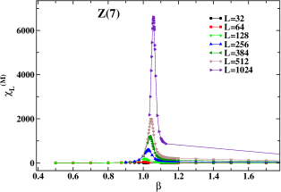
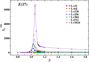
Figure 2: (Color online) Susceptibility $\chi_{L}^{(M)}$ versus $\beta$ in $Z(7)$ (left) and $Z(17)$ (right) on lattices with several values of $L$.

In Fig. 2 we show the behavior of the susceptibility $\chi_{L}^{(M)}\equiv L^{2}(\langle|M_{L}|^{2}\rangle-\langle|M_{L}|\rangle^{2})$ of the absolute value of the complex magnetization, which exhibits, for each volume considered, a clear peak signalling the first phase transition. The position of the peak in the thermodynamic limit defines the first critical coupling, $\beta_{c}^{(1)}$. Fig. 3 shows instead the behavior of $m_{\psi}$ versus $\beta$ on various lattice sizes; here the second critical coupling $\beta_{c}^{(2)}$ is identified by the crossing point (in the thermodynamic limit) of the curves formed by the data on different lattice sizes.

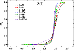
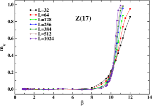
Figure 3: (Color online) Behavior of $m_{\psi}$ with $\beta$ in $Z(7)$ (left) and $Z(17)$ (right) on lattices with several values of $L$.

To determine the first critical coupling $\beta_{c}^{(1)}$, we could extrapolate to infinite volume the pseudo-critical couplings given by the position of the peaks of $\chi_{L}^{(M)}$. However, since the approach to the thermodynamic limit is rather slow (powers of $\log L$), we adopted a different method, based on the use of the “reduced fourth-order” Binder cumulant

$$U^{(M)}_{L}=1-\frac{\langle|M_{L}|^{4}\rangle}{3\langle|M_{L}|^{2}\rangle^{2}}\;,$$ (25)

the cumulant $B_{4}^{(M_{R})}$ defined as

$$B_{4}^{(M_{R})}=\frac{\langle|M_{R}-\langle M_{R}\rangle|^{4}\rangle}{\langle|M_{R}-\langle M_{R}\rangle|^{2}\rangle^{2}}\;,$$ (26)

and the helicity modulus $\Upsilon$. We estimated $\beta_{c}^{(1)}$ by looking for (i) the crossing point of the curves, obtained on different volumes, giving a Binder cumulant versus $\beta$ and (ii) the optimal overlap of the same curves after plotting them versus $(\beta-\beta_{c})(\log L)^{1/\nu}$, with $\nu$ fixed at 1/2. The method (ii) has been applied also to the helicity modulus $\Upsilon$. Our best values for $\beta_{c}^{(1)}$ are

$$N=7: \;\;\;\beta_{c}^{(1)}=1.1113(13)\;,$$

$$N=17: \;\;\;\beta_{c}^{(1)}=1.11375(250)\;.$$

Then, we performed the finite size scaling (FSS) analysis of the magnetization $|M_{L}|$ and the susceptibility $\chi_{L}^{(M)}$ at $\beta_{c}^{(1)}$ using the following laws:

$$|M_{L}|(\beta_{c}^{(1)})=AL^{-\beta/\nu}\;,$$ (27)

$$\chi_{L}^{(M)}(\beta_{c}^{(1)})=BL^{\gamma/\nu}\;,$$ (28)

where $\gamma/\nu=2-\eta$ and $\eta$ is the magnetic critical index. Results are summarized in Tables 4, 5, 6 and 7. We observe that the hyperscaling relation $\gamma/\nu+2\beta/\nu=d=2$ is nicely satisfied within statistical errors in both models.

Table 4: Results of the fit to the data of $|M_{L}|(\beta_{c}^{(1)})$ with the scaling law (27) on $L^{2}$ lattices with $L\geqslant L_{\rm min}$, for $N=7$.

$N=7$
$L_{\rm min}$	$A$	$\beta/\nu$	$\chi^{2}$/d.o.f.
32	1.00653(48)	0.12210(08)	5.5
64	1.00858(70)	0.12243(12)	3.7
128	1.01074(94)	0.12277(15)	2.0
256	1.0146(16)	0.12336(26)	0.40
384	1.0162(22)	0.12359(34)	0.19
512	1.0177(38)	0.12381(56)	0.16
640	1.0185(57)	0.12393(84)	0.28

Table 5: Results of the fit to the data of $|M_{L}|(\beta_{c}^{(1)})$ with the scaling law (27) on $L^{2}$ lattices with $L\geqslant L_{\rm min}$, for $N=17$.

$N=17$
$L_{\rm min}$	$A$	$\beta/\nu$	$\chi^{2}$/d.o.f.
32	1.00388(51)	0.12111(09)	7.98
64	1.00620(69)	0.12149(12)	3.58
128	1.0089(11)	0.12191(18)	1.54
256	1.0107(15)	0.12219(24)	0.74
384	1.0113(24)	0.12228(36)	1.36

Table 6: Results of the fit to the data of $\chi_{L}^{(M)}(\beta_{c}^{(1)})$ with the scaling law (28) on $L^{2}$ lattices with $L\geqslant L_{\rm min}$, for $N=7$.

$N=7$
$L_{\rm min}$	$B$	$\gamma/\nu$	$\chi^{2}$/d.o.f.
32	0.00558(07)	1.7402(23)	2.38
64	0.00540(09)	1.7457(29)	1.32
128	0.00522(12)	1.7508(38)	0.68
256	0.00518(20)	1.7520(61)	0.84
384	0.00546(33)	1.7443(93)	0.70
512	0.00489(52)	1.760(16)	0.28
640	0.00444(76)	1.775(25)	0.0066

Table 7: Results of the fit to the data of $\chi_{L}^{(M)}(\beta_{c}^{(1)})$ with the scaling law (28) on $L^{2}$ lattices with $L\geqslant L_{\rm min}$, for $N=17$.

$N=17$
$L_{\rm min}$	$B$	$\gamma/\nu$	$\chi^{2}$/d.o.f.
32	0.00559(08)	1.7372(26)	2.7
64	0.00532(11)	1.7453(35)	0.39
128	0.00521(15)	1.7484(46)	0.16
256	0.00514(23)	1.7507(71)	0.15
384	0.00522(31)	1.7483(92)	0.13

We can cross-check our determination of the critical exponent $\eta$ by an independent method, which does not rely on the prior knowledge of the critical coupling, but is based on the construction of a suitable universal quantity [17, 11]. The idea is to plot $\chi_{L}^{(M_{R})}L^{\eta-2}$ versus $B_{4}^{(M_{R})}$ and to look for the value of $\eta$ which optimizes the overlap of curves from different volumes. We found that, both in $Z(7)$ and $Z(17)$, $\eta=1/4$ is this optimal value, since it gives the best overlap of these curves in the region of values corresponding to the first phase transition, i.e. the lower branch of the curves of Fig. 4. This result for $\eta$ agrees with the determinations $\eta=2-\gamma/\nu$ from the FSS analysis.

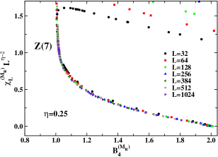
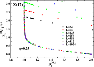
Figure 4: (Color online) Correlation between $\chi_{L}^{(M_{R})}L^{\eta-2}$ and the Binder cumulant $B_{4}^{(M_{R})}$ for $\eta=0.25$ in $Z(7)$ (left) and $Z(17)$ (right) on lattices with $L$ ranging from 128 to 1024.

As for the second critical coupling $\beta_{c}^{(2)}$, we used the same method adopted for $\beta_{c}^{(1)}$, but applied now to $B_{4}^{(M_{R})}$ and $m_{\psi}$. Our best estimates are

$$N=7:\;\;\;\beta_{c}^{(2)}=1.8775(75)\;,\;\;\;\;\;\;\;\;\;\;\;\;\;\;\;N=17:\;\;\;\beta_{c}^{(2)}=10.13(12)\;.$$

The standard FSS analysis applied to the susceptibility $\chi_{L}^{(M_{R})}$ of the rotated magnetization $M_{R}$ at $\beta_{c}^{(2)}$ leads to the result for the critical indices $\gamma/\nu$ given in Tables 8 and 9 .

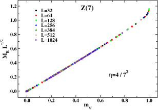
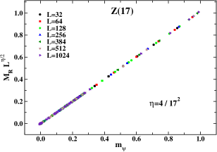
Figure 5: (Color online) Correlation between $M_{R}L^{\eta/2}$ and $m_{\psi}$ for $\eta=4/7^{2}$ in $Z(7)$ (left) and $\eta=4/17^{2}$ in $Z(17)$ (right), on lattices with L ranging from 128 to 1024.

Table 8: Results of the fit to the data of $\chi_{L}^{(M_{R})}(\beta_{c}^{(2)})$ with the scaling law (28) on $L^{2}$ lattices with $L\geqslant L_{min}$, for $N=7$.

$N=7$
$L_{min}$	$A$	$\gamma/\nu$	$\chi^{2}$/d.o.f.
32	0.8767(37)	1.92340(71)	2.02
64	0.8833(47)	1.92219(87)	1.41
128	0.8858(57)	1.9217(11)	1.57
256	0.8997(93)	1.9193(16)	1.02
384	0.916(15)	1.9166(25)	0.68
512	0.921(24)	1.9158(39)	0.98
640	0.942(34)	1.9124(54)	1.07

Table 9: Results of the fit to the data of $\chi_{L}^{(M_{R})}(\beta_{c}^{(2)})$ with the scaling law (28) on $L^{2}$ lattices with $L\geqslant L_{min}$, for $N=17$.

$N=17$
$L_{min}$	$B$	$\gamma/\nu$	$\chi^{2}$/d.o.f.
32	0.9319(47)	1.98933(89)	1.65
64	0.9408(68)	1.9878(12)	1.38
128	0.9533(89)	1.9857(16)	0.67
256	0.954(16)	1.9856(27)	0.83
384	0.950(24)	1.9861(40)	1.09
512	0.931(38)	1.9892(62)	1.44
640	0.911(59)	1.9925(98)	2.67

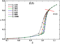
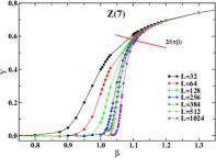
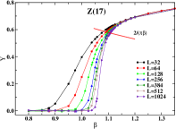
Figure 6: (Color online) Helicity modulus versus $\beta$ in $Z(5)$, $Z(7)$ and $Z(17)$ on lattices with various sizes.

Also in this case the critical index $\eta$ can be determined by an independent method, irrespectively of the knowledge of $\beta_{c}^{(2)}$: $M_{R}L^{\eta/2}$ is plotted versus $m_{\psi}$ and the value of $\eta$ is searched for, which optimizes the overlap of data points coming from different volumes. The results we found for $\eta$ in $Z(7)$ and $Z(17)$ are in perfect agreement with the theoretical prediction $\eta^{(2)}=4/N^{2}$ (see Fig. 5).

Finally, in Fig. 6 we present the behavior with $\beta$ of the helicity modulus (24). This quantity is constructed in such a way that it should exhibit a discontinuous jump (in the thermodynamic limit) at the critical temperature separating the disordered phase from the massless one, if the transition is of infinite order (BKT). Since the Kosterlitz-Thouless RG equations for the $XY$ model [1, 18, 19] lead to the prediction that the helicity modulus $\Upsilon$ jumps from the value $2/(\pi\beta)$ to zero at the critical temperature, one can check if the same occurs for vector Potts models. In Fig. 6 we plot a red line, representing the function $2/(\pi\beta)$; the crossing between this line and the curves formed by data points of $\Upsilon$ approaches indeed $\beta_{c}^{(1)}$ when the lattice size increases.

The knowledge of the behavior with $\beta$ of the helicity modulus provides us with another method for the determination of the critical index $\eta$. As shown in Ref. [19, 20] (see also Ref. [21]), the following relation holds,

$$\eta=\frac{1}{2\pi\beta\Upsilon}\;,$$ (29)

which allows us to get the value of $\eta$ at any fixed $\beta$ in the BKT phase, if the value of $\Upsilon$ at that $\beta$ is known. A simple inspection of the behavior of $\Upsilon$ with $\beta$, shown in Fig. 6, tells us that, for a given $N$, $\eta$ in the BKT phase decreases monotonically from a value compatible with $\eta^{(1)}=1/4$, taken at the first critical coupling $\beta_{c}^{(1)}$, to a value compatible with $\eta^{(2)}=4/N^{2}$, taken at the second critical coupling. In some sense, the $N^{2}$ drop of the value of $\eta$ at the second transition is related to increasing distance between $\beta_{c}^{(2)}$ and $\beta_{c}^{(1)}$.

We studied also the specific heat at the two transitions, finding that, in contrast to the case of first- and second-order phase transitions, it does not reflect any nonanalytical critical properties at the critical temperatures, thus confirming that only BKT transitions are at work here.

4 Behavior with $N$ of the critical couplings

The results of this work and those available in the literature allow us to make some considerations about the behavior with $N$ of the critical coupling $\beta_{c}^{(1)}$ and $\beta_{c}^{(2)}$. Examining Table 1 one concludes that formulae (18) and (19) give the correct qualitative prediction for the scaling of the $\beta_{c}^{(1,2)}$ with $N$ in the Villain formulation. Namely,

• $\beta_{c}^{(1)}$ converges to $XY$ value very fast, like $\exp(-aN^{2})$

• $\beta_{c}^{(2)}$ diverges like $N^{2}$  .

One should expect that the standard vector $Z(N)$ model possesses similar scaling, probably up to ${\cal{O}}(N)$ corrections. One could try therefore to fit available Monte Carlo data for $\beta_{c}^{(1,2)}$ with formulae (18) and (19) modified to account for such corrections.

In Table 10 and in Figs. 7, 8 we summarize the present knowledge about the position of the critical points for $2D$ $Z(N)$ vector models.

Table 10: Summary of the known values of the critical couplings $\beta_{c}^{(1)}$ and $\beta_{c}^{(2)}$ for $2D$ $Z(N)$ vector models.

$N$	$\beta_{c}^{(1)}$	$\beta_{c}^{(2)}$	Reference
5	1.0510(10)	1.1048(10)	[11]
6	1.11012(74)	1.4257(22)	[9]
7	1.1113(13)	1.8775(75)	this work
8	1.11907(88)	2.3480(22)	[9]
12	1.11894(88)	5.0556(128)	[9]
17	1.11375(250)	10.13(12)	this work
$\infty$	1.1199(1)	$\infty$	[22]

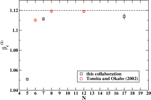
Figure 7: (Color online) Behavior with $N$ of the known values of the critical coupling $\beta_{c}^{(1)}$ in $2D$ $Z(N)$ vector models. The horizontal dashed line represents the critical coupling of $2D$ $XY$, $\beta_{XY}$=1.1199, taken from Ref. [22].

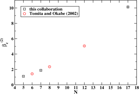
Figure 8: (Color online) Behavior with $N$ of the known values of the critical coupling $\beta_{c}^{(2)}$ in $2D$ $Z(N)$ vector models.

We can see from Fig. 7 that the approach of $\beta_{c}^{(1)}$ to the $N\to\infty$ limit, corresponding to the $2D$ $XY$ model, is indeed very fast. Introducing corrections into the scaling formula (18), we may conjecture the following general behavior:

$$\beta_{c}^{(1)}\ =\ A-(BN^{2}+CN+D)\exp{\left[-\frac{N^{2}}{E}\right]}\ .$$ (30)

Indeed, attempts to fit data with this formula give values for $A$ and $E$ compatible with $\beta_{c}^{XY}$. However, as is seen from Table 10, the combination of our Monte Carlo determinations and those of Ref. [9] leads to a fake non-monotonic approach to $\beta_{c}^{XY}$, in marked contradiction with our RG analysis. Looking separately at the two data sets given in Table 10, one can see that each set indeed satisfies monotonicity (taking into account the error bars in the case of data from Ref. [9]). We think, therefore, that the non-monotonicity of the combined set can be explained with the different systematics affecting the determinations of $\beta_{c}^{(1)}$ by the two collaborations. On our side, we have determined the location of $\beta_{c}^{(1)}$ by two different methods, using several observables and working on larger lattices, up to $L=1024$, thus making us very confident on the reliability of our results. In conclusion, a reliable check of the formula (30), based on all data given in Table 10, is not possible and that formula remains a conjecture.

In the case of $\beta_{c}^{(2)}$, instead, one can verify that, for example, the following extension of (19)

$$\beta_{c}^{(2)}\ =\ \frac{N^{2}}{A}+BN+C+De^{-\frac{\pi^{2}N^{2}}{A}}$$ (31)

fits the data rather well, although with a high $\chi^{2}$/d.o.f. probably reflecting the different systematics mentioned above,

$$A\ =\ 25.89(115)\ ,\;\;\;B\ =\ -0.040(23)\ ,\;\;\;C\ =\ 0.38(9)\ ,\;\;\;D\ =\ 227.7(634)\ ,\;\;\;\chi^{2}\ =\ 12.69\ .$$

The value of $A$ is close to $8\pi$, as is expected.

In general, however, we have to conclude that even if the scaling formulae (30) and (31) might be correct, more data for different $N$ are needed to determine all coefficients.

5 Summary

In this paper we have studied the RG equations describing the critical behavior of $2D$ $Z(N)$ vector models in the Villain formulation. The main original results are

• the RG trajectories in the vicinity of both phase transitions,

• the critical points as functions of $N$,

• the index $\nu$, which turns out to be equal to 1/2 for all $N>4$.

The numerical part of the work has been devoted to verify these theoretical expectations:

• We have determined numerically the two critical couplings of the $2D$ $Z(N=7,17)$ vector models and given estimates of the critical indices $\eta$ at both transitions. Our findings support for all $N\geq 5$ the standard scenario of three phases: a disordered phase at high temperatures, a massless or BKT one at intermediate temperatures and an ordered phase, occurring at lower and lower temperatures as $N$ increases. This matches perfectly with the $N\to\infty$ limit, i.e. the $2D$ $XY$ model, where the ordered phase is absent or, equivalently, appears at $\beta\to\infty$.

• We have found that the values of the critical index $\eta$ at the two transitions are compatible with the theoretical expectations.

• The index $\nu$ also appears to be compatible with the value $1/2$, in agreement with RG predictions.

On the basis of this study and taking into account previous works [9, 11], we are prompted to conclude that $2D$ $Z(N)$ vector models in the standard formulation undergo two phase transitions of the BKT type. Furthermore, the standard and the Villain formulations belong to the same universality class with $\nu=1/2$, $\eta^{(1)}=1/4$ and $\eta^{(2)}=4/N^{2}$.

Considering the determinations of the critical couplings as a function of $N$, we have calculated the leading dependences using RG equations and conjectured the approximate scaling for $\beta_{c}^{(1,2)}(N)$ in the standard version. The existing numerical values and their accuracy are not sufficient, however to reliably check the conjectured formulae.

6 Acknowledgments

The work of G.C. and M.G. was supported in part by the European Union under ITN STRONGnet (grant PITN-GA-2009-238353).

References

- [1] V. Berezinskii, Sov. Phys. JETP 32 (1971) 493.
- [2] J. Kosterlitz, D. Thouless, J. Phys. C6 (1973) 1181; J. Kosterlitz, J. Phys. C7 (1974) 1046.
- [3] O. Borisenko, M. Gravina, A. Papa, J. Stat. Mech. 2008 (2008) P08009 [arXiv:0806.2081 [hep-lat]].
- [4] O. Borisenko, R. Fiore, M. Gravina, A. Papa, J. Stat. Mech. 2010 (2010) P04015 [arXiv:1001.4979 [hep-lat]].
- [5] O. Borisenko, G. Cortese, R. Fiore, M. Gravina, A. Papa, PoS LATTICE2011 (2011) 304 [arXiv:1110.6385 [hep-lat]].
- [6] S. Elitzur, R.B. Pearson, J. Shigemitsu, Phys. Rev. D19 (1979) 3698.
- [7] M.B. Einhorn, R. Savit, A physical picture for the phase transitions in -symmetric models, Preprint UM HE 79-25; C.J. Hamer, J.B. Kogut, Phys. Rev. B22 (1980) 3378; B. Nienhuis, J. Statist. Phys. 34 (1984) 731; L.P. Kadanoff, J. Phys. A11 (1978) 1399.
- [8] J. Fröhlich, T. Spencer, Commun. Math. Phys. 81 (1981) 527.
- [9] Y. Tomita, Y. Okabe, Phys. Rev. B65 (2002) 184405.
- [10] O. Borisenko, G. Cortese, R. Fiore, M. Gravina, A. Papa, PoS(Lattice 2010)274 [arXiv:1101.0512 [hep-lat]].
- [11] O. Borisenko, G. Cortese, R. Fiore, M. Gravina, A. Papa, Phys. Rev. E83 (2011) 041120 [arXiv:1011.5806 [hep-lat]].
- [12] S.K. Baek and P. Minnhagen, Phys. Rev. E 82 (2010) 031102 [arXiv:1009.0356 [cond-mat.stat-mech]].
- [13] W. Janke and K. Nather, Phys. Rev. B48 (1993) (7419); M. Hasenbusch and K. Pinn, J. Phys. A30 (1997) 63.
- [14] P. Minnhagen, B.J. Kim, Phys. Rev. B67 (2003) 172509 [arXiv:cond-mat/0304226 [cond-mat.supr-con]].
- [15] M. Hasenbusch, J. Stat. Mech. (2008) P08003 [arXiv:0804.1880v1 [cond-mat.stat-mech]].
- [16] S.K. Baek, P. Minnhagen and B.J. Kim, Phys. Rev. E80 (2009) 060101(R) [arXiv:0912.2830v1 [cond-mat.stat-mech]].
- [17] D. Loison, J. Phys.: Condens. Matter 11 (1999) L401.
- [18] T. Ohta and D. Jasnow, Phys. Rev. B20 (1979) 139.
- [19] D.R. Nelson and J.M. Kosterlitz, Phys. Rev. Lett. 39 (1977) 1201.
- [20] J.E. van Himbergen, J. Phys. C17 (1984) 5039.
- [21] A. Yamagata and I. Ono, J. Phys. A24 (1991) 265.
- [22] M. Hasenbusch, J. Phys. A 38 (2005) 5869 [arXiv:cond-mat/0502556v2 [cond-mat.stat-mech]].