Exact Method for Determining Subsurface Radioactivity Depth Profiles from Gamma Spectroscopy Measurements

Abstract

Subsurface radioactivity may be due to transport of radionuclides from a contaminated surface into the solid volume, as occurs for radioactive fallout deposited on soil, or from fast neutron activation of a solid volume, as occurs in concrete blocks used for radiation shielding. For purposes including fate and transport studies of radionuclides in the environment, decommissioning and decontamination of radiation facilities, and nuclear forensics, an in situ, nondestructive method for ascertaining the subsurface distribution of radioactivity is desired. The method developed here obtains a polynomial expression for the radioactivity depth profile, using a small set of gamma-ray count rates measured by a collimated detector directed towards the surface at a variety of angles with respect to the surface normal. To demonstrate its capabilities, this polynomial method is applied to the simple case where the radioactivity is maximal at the surface and decreases exponentially with depth below the surface, and to the more difficult case where the maximal radioactivity is below the surface.

I Introduction

Nondestructive methods to determine the extent of subsurface radioactivity rely on the attenuation of characteristic gamma-rays emitted from the subsurface. Assuming the radionuclide distribution is reasonably uniform in the two dimensions parallel to the surface, the problem reduces to finding the (one-dimensional) depth profile of the radioactivity. To accomplish this, two general approaches have been taken: (i) A depth distribution function is assumed (from physical considerations), and spectroscopic measurements are made to determine the best-fit values for the function parameters. (ii) No depth distribution is assumed; rather, the subsurface volume is divided into voxels, and spectroscopic measurements are made to determine the activity of each voxel.

Often there is good reason to assume a particular depth distribution function. For example, Smith and Elder [1] consider several parameterized functions based on physical processes related to radionuclide mobility in soils. The review by MacDonald et al. [2] discusses three spectroscopic methods used to obtain the function parameters: (i) The “multiple peak method”, which uses the fact that the scatter cross-section of a gamma-ray is a function of its energy (so for example, the two parameters of an exponential decay function representing the radionuclide distribution are calculated from measurements of the count rates of two characteristic gamma-rays of different energy). (ii) The “peak to valley method”, which uses the fact that the ratio of counts in a characteristic gamma-ray peak to counts in the adjacent “valley” of slightly lower energy (due to forward scattering of the characteristic gamma-rays) decreases with increased attenuation of the characteristic gamma-rays (e.g. Gering et al. [3] who use a two-parameter Lorentz function for ¹³⁷Cs in soil). (iii) The “lead plate method”, where an absorbing lead plate inserted between the detector and the material surface allows the flux contribution from large angle (with respect to the surface normal) to be distinguished from that from small angle (e.g., Korun et al. [4] who use a three-parameter Gaussian function for ¹³⁷Cs and ¹³⁴Cs in soil; Dewey et al. [5] who fit a variety of analytical functions to simulated measurements for ¹³⁷Cs in soil; Benke and Kearfott [6],[7] who consider planar radiation sources at various depths).

When a particular depth distribution cannot be assumed, or none of a set of parameterized functions can be well matched to the spectroscopic measurements, the subsurface volume may be (virtually) divided into voxels, and the activity of each voxel determined by some variation of the following procedure. Count rates of a characteristic gamma-ray are obtained by a collimated detector directed at (or otherwise sensitive only to gamma-rays emitted at) particular angles $\theta$ with respect to the surface normal. By obtaining count rates for a number of different detector orientations, the response matrix equation $C=\mathbf{R}\Lambda$ can be constructed, where element $c_{i}$ of vector $C$ is the count rate obtained for angle $\theta_{i}$, the detector response matrix element $r_{ij}$ is the probability that a gamma-ray emitted from voxel $j$ will contribute to the count rate $c_{i}$ (so $r_{ij}$ accounts for scattering of that gamma-ray en route to the detector), and element $a_{j}$ of vector $\Lambda$ is the activity of voxel $j$. Given the vector $C$, the matrix equation is solved for the activity vector $\Lambda$. This “voxel approach” is taken by, e.g., Benke et al. [8],[9]; Whetstone et al. [10]; Charles et al. [11].

These approaches to finding the radioactivity depth profile are not entirely satisfactory for the following reasons. In the case of the “parameterized function approach”, the assumption of a particular depth distribution function is risky in general, even when best-fit parameter values are found that seem to bear out the assumption. By the nature of the measurements, the candidate functions are limited to those with very few parameters, so reasonable best-fit parameter values may be found for more than one of those functions. In the case of the “voxel approach”, the limited number of spectroscopic measurements greatly limits the number of voxels into which the subsurface is divided. In any event, the calculated activity $a_{j}$ (gamma-ray emissions per unit time) is evenly distributed over the entire volume of voxel $j$, so giving the calculated distribution a spatial resolution no better than the voxel size.

The new approach presented below is motivated by the expectation that the “true” depth profile function is smooth and continuous. Thus it can be closely approximated by a polynomial expression, with more or fewer terms depending on the complexity of the “true” function (for example, more terms are needed to approximate a Gaussian-like function than an exponential-like function). The success of this method is due to the novel way the coefficients of the terms in the polynomial are obtained from the spectroscopic measurements.

II Calculation of the polynomial profile function

For convenience, the surface is at $z=0$ and the radioactive material lies in the region $z\geq 0$. In what follows, $\rho(z)dV$ is the activity (number of gamma-rays emitted per second) of the infinitesimal volume $dV$ located in the subsurface layer $\left[z,z+dz\right]$; thus the distribution $\rho(z)$ is the activity per unit volume at depth $z$.

This “polynomial method” is most easily developed by considering the idealized case of a highly collimated, one-pixel gamma-ray detector pointing at the material surface. Due to the collimation, only those characteristic gamma-rays emitted from a thin “pencil” of material will be counted at the detector. Unless all radioactivity is on the surface, the detector counts will provide an underestimate of the total activity, due to attenuation (scattering) of the subsurface emissions. Different orientations of the detector with respect to the surface normal will thus produce different count rates, due to the different orientations of the pencil of material with respect to the subsurface radioactivity profile. As shown below, that radioactivity profile can be ascertained from the variation in count rate with detector orientation.

Consider that the highly collimated, one-pixel detector is pointing at the surface at an angle $\theta$ from the surface normal. The collimation ensures that all recorded characteristic gamma-rays originate from the thin pencil of material angled by $\theta$ with respect to the surface normal. Note that a gamma-ray emitted at depth $z$ and recorded at the detector has travelled a distance $z/\cos\theta$ to the surface. Thus the count rate $d(\theta)$ recorded at the detector is given by

$$d\left(\theta\right)=\varepsilon\int\limits_{z=0}^{z=\infty}\rho(z)\frac{A}{4\pi\left(\frac{z+R}{\cos\theta}\right)^{2}}\exp\left[-\mu\left(\frac{z}{\cos\theta}\right)\right]\frac{A}{\cos\theta}dz$$ (1)

where the (unknown) function $\rho(z)$ is the activity per unit volume at depth $z$; $\mu$ is the attenuation coefficient for the characteristic gamma-ray in the homogeneous material (attenuation in air is ignored); $R$ is the normal distance of the pixel center above the surface; $A$ is the cross-sectional area of the pencil volume, as well as the area of the detector pixel; and $\varepsilon$ is the detector efficiency (possibly multiplied by factors related to the system geometry and instrument characteristics). Note that the integration is over all infinitesimal volumes $dV=dz\cdot A/\cos\theta$ comprising the pencil volume. The ratio $A\left[4\pi\left(\frac{z+R}{\cos\theta}\right)^{2}\right]^{-1}$ is the fraction of emissions from the volume $dV$ that would reach the detector in the absence of attenuation, while the exponential factor accounts for the attenuation.

When count rates are obtained for several different detector orientations (several different $\theta$ values), a set of these integral equations is created, which in principle can be solved for the unknown radioactivity profile $\rho(z)$. The approach taken here is to approximate $\rho(z)$ by the polynomial $\rho^{\ast}(z)$ of degree $N$,

$$\rho^{\ast}(z)=\sum\limits_{j=0}^{N}c_{j}\cdot z^{j}=c_{0}+c_{1}z+c_{2}z^{2}+\ldots+c_{N}z^{N}$$ (2)

where the coefficients $c_{j}$ are determined from the detector count rates in the following manner.

Each detector orientation with respect to the surface normal produces a linear equation

$$d_{i}=\sum\limits_{j=0}^{N}K_{ij}c_{j}$$ (3)

where $d_{i}$ is the count rate $d\left(\theta_{i}\right)$, as the index $i$ distinguishes the different detector orientations; and the coefficients

$$K_{ij}=\varepsilon\int\limits_{z=0}^{z=\zeta}z^{j}\frac{A}{4\pi\left(\frac{z+R}{\cos\theta_{i}}\right)^{2}}\exp\left[-\mu\left(\frac{z}{\cos\theta_{i}}\right)\right]\frac{A}{\cos\theta_{i}}dz\text{.}$$ (4)

Note that the limit of integration $\zeta$ is the depth below which no radioactivity is present; this is a parameter that must be set (i.e., assumed) prior to the calculations. In the case of $n$ detector orientations, $n$ equations like Eq. (3) are created. Two additional linear equations are needed to force the function $\rho^{\ast}(z)$ to go smoothly to zero at $z=\zeta$. These are

$$d_{n}=0=\sum\limits_{j=0}^{N}K_{n,j}c_{j}$$ (5)

where the coefficients $K_{n,j}=\zeta^{j}$ [this is just the equation $\rho^{\ast}(\zeta)=0$], and

$$d_{n+1}=0=\sum\limits_{j=0}^{N}K_{n+1,j}c_{j}$$ (6)

where the coefficients $K_{n+1,j}=j\cdot\zeta^{j-1}$ [this is the equation $d\rho^{\ast}(z)/dz=0$ at $z=\zeta$, which ensures the slope of $\rho^{\ast}(z)$ is zero at $z=\zeta$].

The set of $n+2$ linear equations is then solved for the set $\left\{c_{j}\right\}$, thus producing the radioactivity profile $\rho^{\ast}(z)$ according to Eq. (2). This function reproduces the set $\left\{d_{i}\right\}$ of count-rate measurements, and goes smoothly to zero at $z=\zeta$.

Note that the total activity $\Lambda_{T}$ (number of characteristic gamma-rays emitted per second) of a “core” of cross-sectional area $A$ (taken perpendicular to the surface) is

$$\Lambda_{T} =A\int\limits_{z=0}^{z=\infty}\rho(z)dz$$

$$\approx A\int\limits_{z=0}^{z=\zeta}\rho^{\ast}(z)dz=A\sum\limits_{j=0}^{N}\frac{c_{j}}{j+1}\zeta^{j+1}\text{.}$$ (7)

The activity of any slice of that core is obtained by integrating $\rho^{\ast}(z)$ over the thickness of that slice.

A computational caution: When the integrals in Eq. (4) are evaluated to obtain the set $\left\{K_{ij}\right\}$, it may be found that those values range over several orders of magnitude. This makes it exceedingly difficult to solve the system of $n+2$ equations for the set $\left\{c_{j}\right\}$ by conventional methods. Thus an analytical, “term elimination sequence” method for solving a square system of linear equations was derived for this purpose. It is presented in the appendix in a form that is very easy to write into a computer code. All of the polynomial functions plotted in the following section were obtained by use of this method incorporated into a simple Mathematica code.

After this exposition of the polynomial method, it is interesting to briefly consider the “voxel approach” to determining the radioactivity depth profile mentioned in Section I. The set $\left\{d_{i}\right\}$ of count-rate measurements is related to the set $\left\{a_{j}\right\}$ of voxel activities by a set of linear equations of the sort

$$d_{i}=\sum\limits_{j=0}^{N}R_{ij}a_{j}$$ (8)

where the $N+1$ voxels are each of size $A\cdot\delta z$ and the dimensionless coefficients

$$R_{ij}=\varepsilon\frac{A}{4\pi\left(\frac{\delta z\cdot j+R}{\cos\theta_{i}}\right)^{2}}\exp\left[-\mu\left(\frac{\delta z\cdot j}{\cos\theta_{i}}\right)\right]\frac{1}{\cos\theta_{i}}\text{.}$$ (9)

Clearly the number of voxels cannot exceed the number of measurements (detector orientations), and the voxel thickness $\delta z\gg dz$ must be sufficient that the array of voxels fills the assumed radioactive volume. Of course, the polynomial method completely avoids discretization of that volume.

III Application of the polynomial method

Unfortunately, the functional requirements on $\rho^{\ast}(z)$ that it be continuous, go smoothly to zero at some depth $\zeta$, and reproduce the spectroscopic measurements $\left\{d_{i}\right\}$, do not automatically ensure that the unknown radioactivity profile function $\rho(z)$ is reproduced. The finite number of terms in the polynomial (limited by the number of measurements taken) may be insufficient to produce a complex function, or the finite depth $\zeta$ at which radioactivity is presumed negligible may be poorly chosen. Indeed, the exponential decay function, which is a typical radioactivity profile, is actually a polynomial with an infinite number of terms that goes to zero at infinity.

But fortunately, non-physical (nonsensical) $\rho^{\ast}(z)$ functions are easy to distinguish visually. In addition to the functional requirements on $\rho^{\ast}(z)$, the areas under the curves $\rho^{\ast}(z)$ and $\rho(z)$ are approximately equal [see Eq. (7)]. Thus either the curve $\rho^{\ast}(z)$ closely tracks the curve $\rho(z)$, or the constraints are accommodated by anomalous undulations of the curve $\rho^{\ast}(z)$. Examples of this behavior are evident in Fig. 1,

Figure 1: Fourth-degree polynomial representations of the radioactivity depth profile $\rho\left(z\right)=\exp\left[-z/0.003\right]$ (the thickest curve). The odd curve is $\rho^{\ast}\left(z\right)$ that terminates at $\zeta=0.01$; the $\rho^{\ast}\left(z\right)$ curves for $\zeta=0.015,0.02,0.025$ track the $\rho\left(z\right)$ curve fairly well. All the $\rho^{\ast}\left(z\right)$ curves are calculated from the count-rate measurements $\left\{d\left(i\frac{\pi}{16}\right)\right\}$.

where the radioactivity profile $\rho(z)=\exp[-z/0.003]$ is approximated by a 4th degree polynomial calculated from count-rate measurements at three detector orientations $\theta=0,\pi/16,\pi/8$. The four curves are $\rho^{\ast}(z)$ obtained for $\zeta=0.01,0.015,0.02,0.025$, respectively. Clearly the curve obtained for $\zeta=0.01$ is physically unlikely due to its hump, while the curve obtained for $\zeta=0.025$ actually goes slightly negative. In contrast, the curves obtained for $\zeta=0.015$ and $0.02$ look physically reasonable. Figures 2

Figure 2: Fifth-degree polynomial representations of the radioactivity depth profile $\rho\left(z\right)=\exp\left[-z/0.003\right]$ (the thickest curve). The $\rho^{\ast}\left(z\right)$ curve is actually three indistinguishable curves (for $\zeta=0.015$) calculated from count-rate measurements $\left\{d\left(i\frac{\pi}{20}\right)\right\},\left\{d\left(i\frac{\pi}{16}\right)\right\},\left\{d\left(i\frac{\pi}{12}\right)\right\}$, respectively.

and 3

Figure 3: Similar to Fig. 2, but the three indistinguishable $\rho^{\ast}\left(z\right)$ curves terminate at $\zeta=0.02$ rather than at $\zeta=0.015$. The absence of the non-physical hump evident in the curves of Fig. 2 suggests that the 5th degree polynomial $\rho^{\ast}\left(z\right)$ for $\zeta=0.02$ is a good representation of the radioactivity depth profile $\rho\left(z\right)$.

show the 5th degree polynomial $\rho^{\ast}(z)$ for $\zeta=0.015$ and $0.02$, respectively. Each figure shows three curves (impossible to distinguish since they’re essentially identical); each curve is calculated from count-rate measurements at detector orientations $\theta=0,\varphi,2\varphi,3\varphi$, where $\varphi$ is $\pi/20,\pi/16,\pi/12$ for the three curves, respectively. The $\rho^{\ast}(z)$ curves in Fig. 2 are physically unlikely (due to the hump), while there is nothing objectionable about the $\rho^{\ast}(z)$ curves in Fig. 3. Thus any one of the three 5th degree polynomials (for $\zeta=0.02$) shown in Fig. 3 should be a good match to the unknown profile function $\rho(z)$, as in fact is the case.

Note that the sets $\left\{d_{i}\right\}$ [AKA $\left\{d\left(\theta_{i}\right)\right\}$] of count-rate measurements used to produce the polynomial curves in these (and following) figures are obtained by solving Eq. (1) for various values of the detector orientation $\theta$. To specify those angles, it is convenient to use the notation $\left\{d\left(i\frac{\pi}{12}\right)\right\}_{i=0,\ldots,N-2}$ (for example) or just $\left\{d\left(i\frac{\pi}{12}\right)\right\}$ when the degree $N$ of the polynomial is otherwise noted (the degree of the polynomial is the number of detector orientations plus $1$). Also, the calculations use the attenuation coefficient $\mu=18$ m^-1 appropriate for the $662$ keV gamma-ray emitted by ¹³⁷Cs in concrete; detector-surface separation $R=0.02$ m; detector pixel area $A=\left(0.005\right)^{2}$ m²; detector efficiency $\varepsilon=1$.

A more challenging case is that of the radioactivity profile $\rho\left(z\right)=z\exp\left[-z/0.003\right]$, which goes steeply to zero at the material surface. A profile of this general shape may occur for neutron activated concrete shielding, due to thermalization and subsequent capture of fast neutrons incident on the concrete blocks (Kimura et al. [12], Masumoto et al. [13], Wang et al. [14]). Figure 4

Figure 4: Fourth-degree polynomial representations of the radioactivity depth profile $\rho\left(z\right)=z\exp\left[-z/0.003\right]$ (the thickest curve). The $\rho^{\ast}\left(z\right)$ curve is actually three indistinguishable curves (for $\zeta=0.025$) calculated from count-rate measurements $\left\{d\left(i\frac{\pi}{20}\right)\right\},\left\{d\left(i\frac{\pi}{16}\right)\right\},\left\{d\left(i\frac{\pi}{12}\right)\right\}$, respectively.

shows three (impossible to distinguish) 4th degree polynomials $\rho^{\ast}(z)$ for $\zeta=0.025$ (other, similar calculations showed the appropriate value for $\zeta$ to be $0.02<\zeta<0.03$) calculated from count-rate measurements $\left\{d\left(i\frac{\pi}{20}\right)\right\},\left\{d\left(i\frac{\pi}{16}\right)\right\},\left\{d\left(i\frac{\pi}{12}\right)\right\}$, respectively. These results show convincingly that the radioactivity is maximal below the surface, but one might wonder about the behavior very close to the surface, as a 4th degree polynomial has too few terms to effect a tight bend down to a very low surface value. Figure 5

Figure 5: Similar to Fig. 4, but the three $\rho^{\ast}\left(z\right)$ curves are fifth-degree polynomials.

shows the corresponding 5th degree polynomials $\rho^{\ast}(z)$, all of which go nearly to zero at the material surface.

It is interesting to consider higher-degree (beyond 5th) polynomial approximations to the profile function $\rho\left(z\right)=z\exp\left[-z/0.003\right]$ for their cautionary tales, even though it may be difficult to get more than four distinct measurements $d_{i}$ in practice. Figure 6

Figure 6: Similar to Figs. 4 and 5, but the three $\rho^{\ast}\left(z\right)$ curves are sixth-degree polynomials. The wildly undulating curves calculated from measurements $\left\{d\left(i\frac{\pi}{20}\right)\right\}$ and $\left\{d\left(i\frac{\pi}{16}\right)\right\}$ are clearly non-physical. In contrast, the reasonable behavior of the $\rho^{\ast}\left(z\right)$ curve calculated from the measurements $\left\{d\left(i\frac{\pi}{12}\right)\right\}$ suggests that it is a good representation of the radioactivity depth profile $\rho\left(z\right)$.

shows the corresponding 6th degree polynomials $\rho^{\ast}(z)$. That calculated from the measurement set $\left\{d\left(i\frac{\pi}{12}\right)\right\}$ tracks the $\rho\left(z\right)$ curve very nicely; the others are physically impossible! Figures 7

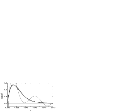
Figure 7: Similar to Figs. 4–6, but the three $\rho^{\ast}\left(z\right)$ curves are seventh-degree polynomials. The wildly undulating curve is calculated from the measurements $\left\{d\left(i\frac{\pi}{20}\right)\right\}$ (note that it closely resembles the corresponding curve in Fig. 6).

and 8

Figure 8: Similar to Figs. 4–7, but the two $\rho^{\ast}\left(z\right)$ curves are eighth-degree polynomials. Again, the wildly undulating curve is calculated from the measurements $\left\{d\left(i\frac{\pi}{20}\right)\right\}$, while the reasonable curve is calculated from the measurements $\left\{d\left(i\frac{\pi}{16}\right)\right\}$.

show the corresponding 7th and 8th degree polynomials $\rho^{\ast}(z)$, respectively. Clearly, use of the set $\left\{d\left(i\frac{\pi}{12}\right)\right\}$ is preferable, presumably due to its wider range of values (of course, all detector orientations must have $\theta<\pi/2$).

The polynomial method also handles the case of a uniform radioactivity distribution $\rho(z)=1$, as occurs for natural radioactivity in soils for example. Figure 9

Figure 9: Fourth-degree polynomial representations of the uniform radioactivity depth profile $\rho\left(z\right)=1$ (the thickest curve). The $\rho^{\ast}\left(z\right)$ curves for $\zeta=0.15,0.5,1,2$ are calculated from the count-rate measurements $\left\{d\left(i\frac{\pi}{16}\right)\right\}$.

shows the 4th degree polynomials $\rho^{\ast}(z)$ for $\zeta=0.15,0.5,1,2$ calculated from count-rate measurements $\left\{d\left(i\frac{\pi}{16}\right)\right\}$. From visual inspection of the curves, it is clear that the polynomial $\rho^{\ast}(z)\rightarrow\rho(z)$ as $\zeta\rightarrow\infty$.

IV Use of multi-pixel detectors

While a “highly collimated, one-pixel gamma-ray detector” is used in Section II to simplify the presentation of the method, in practice a collimated detector with many pixels is needed to accumulate sufficient counts in a reasonable time. Recall that collimation is necessary so that each pixel records only characteristic gamma-rays emitted at a particular angle $\theta$ with respect to the surface normal. This is perhaps most easily accomplished by a collimator that is a thick sheet of lead with a set of parallel holes (say, $M$ in number) drilled through it. This effectively converts a standard detector into an array of $M$ collimated, single-pixel detectors (the single pixel is the size of the hole cross-section). Of course, there being only a single detector behind the perforated lead collimator, only a total gamma-ray count is acquired; that is, the sum of the contributions of the $M$ single-pixel detectors is obtained.

Use of such a detector is easily accommodated by the mathematical development in Section II. In particular, the count rate $d_{i}$ [AKA $d\left(\theta_{i}\right)$, to make clear that the subscript $i$ identifies the particular value of $\theta$] in Eq. (3) is then the total counts recorded at the detector (that is, the sum of the contributions of the $M$ single-pixel detectors) over the time period, and Eq. (4) for the coefficients $K_{ij}$ becomes

$$K_{ij} =\varepsilon\int\limits_{z=0}^{z=\zeta}z^{j}\left[\sum\limits_{m=1}^{M}\frac{A}{4\pi\left(\frac{z+R_{i}^{(m)}}{\cos\theta_{i}}\right)^{2}}\right]$$

$$\exp\left[-\mu\left(\frac{z}{\cos\theta_{i}}\right)\right]\frac{A}{\cos\theta_{i}}dz$$ (10)

where $R_{i}^{(m)}$ is the normal distance of pixel $m$ above the surface.

V Incorporation of known surface conditions

The polynomial method is intended for use when the “true” radioactivity depth profile $\rho\left(z\right)$ is unknown. However, it is conceivable that the activity at the material surface is known (via a swipe test or a shallow core, for example), thus giving a value for the coefficient $c_{0}$. Then Eq. (3) is written

$$d_{i}-K_{i0}c_{0}=\sum\limits_{j=1}^{N}K_{ij}c_{j}$$ (11)

which is conveniently expressed as

$$\delta_{i}=\sum\limits_{j=1}^{N}K_{ij}c_{j}$$ (12)

where $\delta_{i}\equiv d_{i}-K_{i0}c_{0}$ and the index $i$ runs from $1$ to $N$, so that the term elimination sequence method (see appendix) can be used to solve the system of equations for the coefficients $c_{1},\ldots,c_{N}$. In the case of the radioactivity profile $\rho\left(z\right)=z\exp\left[-z/0.003\right]$ considered above, prior knowledge that $c_{0}=0$ would allow Eq. (12) to be used, with count-rate measurements $\left\{d\left(\left(i-1\right)\frac{\pi}{12}\right)\right\}_{i=1,\ldots,N-2}$, say.

Similarly, the slope $c_{1}$ of the radioactivity profile at the surface may be known as well (for example, buried radionuclides would have $c_{0}=c_{1}=0$), so Eq. (3) is expressed as

$$\delta_{i}=\sum\limits_{j=2}^{N}K_{ij}c_{j}$$ (13)

where $\delta_{i}\equiv d_{i}-K_{i0}c_{0}-K_{i1}c_{1}$ and the index $i$ runs from $2$ to $N$, and again the term elimination sequence method of solution can be used.

VI Concluding remarks

The expectation that the radioactivity depth profile is continuous and smooth leads to the “polynomial method” for determining that profile. Values for the coefficients of the terms in the polynomial are obtained in a clever way from a set of characteristic gamma-ray count-rate measurements such that the polynomial function exactly reproduces the measurements. Practical virtues of this approach include (i) it is non-destructive, (ii) no a priori assumptions regarding the functional form of the radioactivity depth profile are needed, and (iii) very few spectroscopic measurements are needed. In contrast, current non-destructive approaches assume a particular radioactivity depth profile function (which is then fitted to the measurements) or divide the subsurface volume into a small number of voxels (which cannot exceed the number of distinct measurements).

The polynomial method is particularly well suited to ascertaining the depth distribution of subsurface radioactivity due to neutron activation of radiation shielding (Kimura et al. [12], Masumoto et al. [13], Wang et al. [14], Žagar and Ravnik [15]) and structural materials (Nakanishi et al. [16]). Thus important applications are to decommissioning and decontamination of accelerators and other radiation facilities (e.g., enabling separation of radioactive portions from larger volumes), and nuclear forensics (e.g., determining the neutron fluence and energy spectrum after a nuclear event).

Appendix: Term elimination sequence method for solution of systems of linear equations

After obtaining the set $\left\{d_{i}\right\}$ of count-rate measurements and calculating the set $\left\{K_{ij}\right\}$ of coefficients, the system of equations of the sort Eq. (3) must be solved for the set $\left\{c_{j}\right\}$. Note that

$$d_{i}=\sum\limits_{j=0}^{N}K_{ij}c_{j}=K_{iN}c_{N}+\sum\limits_{j=0}^{N-1}K_{ij}c_{j}$$

$$\Rightarrow\frac{d_{N}}{K_{NN}}-\frac{d_{i}}{K_{iN}}=\sum\limits_{j=0}^{N-1}\left(\frac{K_{Nj}}{K_{NN}}-\frac{K_{ij}}{K_{iN}}\right)c_{j}$$

$$\text{with }i,j\leq N-1\text{.}$$ (14)

This last equation can be written

$$q_{i}=\sum\limits_{j=0}^{N-1}Q_{ij}c_{j}\text{ where }q_{i}\equiv\frac{d_{N}}{K_{NN}}-\frac{d_{i}}{K_{iN}}\text{ and}$$

$$Q_{ij}\equiv\frac{K_{Nj}}{K_{NN}}-\frac{K_{ij}}{K_{iN}}\text{ with }i,j\leq N-1\text{.}$$ (15)

Clearly this two-step procedure can be repeated until the number of terms in the summation is reduced to one. This suggests the following method of solution.

Consider the (square) system of linear equations of the sort

$$q_{i}^{(N)}=\sum\limits_{j=0}^{N}Q_{ij}^{(N)}c_{j}$$ (16)

where the superscripts on the quantities $q_{i}$ and $Q_{ij}$ are intended only to distinguish the sets $\left\{q_{i}^{(N)},Q_{ij}^{(N)}\right\}$, $\left\{q_{i}^{(N-1)},Q_{ij}^{(N-1)}\right\}$, etc., as needed below. The quantities $q_{i}^{(N)}$ and $Q_{ij}^{(N)}$ correspond to $d_{i}$ and $K_{ij}$, respectively, so the set $\left\{q_{i}^{(N)},Q_{ij}^{(N)}\right\}_{0\leq i,j\leq N}$ is already known. Then according to the two-step procedure above,

$$q_{i}^{(N-1)}\equiv\frac{q_{N}^{(N)}}{Q_{NN}^{(N)}}-\frac{q_{i}^{(N)}}{Q_{iN}^{(N)}}\text{ and}$$

$$Q_{ij}^{(N-1)}\equiv\frac{Q_{Nj}^{(N)}}{Q_{NN}^{(N)}}-\frac{Q_{ij}^{(N)}}{Q_{iN}^{(N)}}\text{ with }i,j\leq N-1$$ (17)

$$q_{i}^{(N-2)}\equiv\frac{q_{N-1}^{(N-1)}}{Q_{N-1,N-1}^{(N-1)}}-\frac{q_{i}^{(N-1)}}{Q_{i,N-1}^{(N-1)}}\text{ and}$$

$$Q_{ij}^{(N-2)}\equiv\frac{Q_{N-1,j}^{(N-1)}}{Q_{N-1,N-1}^{(N-1)}}-\frac{Q_{ij}^{(N-1)}}{Q_{i,N-1}^{(N-1)}}\text{ with }i,j\leq N-2$$ (18)

$$\vdots$$

$$q_{i}^{(1)}\equiv\frac{q_{2}^{(2)}}{Q_{22}^{(2)}}-\frac{q_{i}^{(2)}}{Q_{i2}^{(2)}}\text{ and}$$

$$Q_{ij}^{(1)}\equiv\frac{Q_{2j}^{(2)}}{Q_{22}^{(2)}}-\frac{Q_{ij}^{(2)}}{Q_{i2}^{(2)}}\text{ with }i,j\leq 1$$ (19)

$$q_{i}^{(0)}\equiv\frac{q_{1}^{(1)}}{Q_{11}^{(1)}}-\frac{q_{i}^{(1)}}{Q_{i1}^{(1)}}\text{ and}$$

$$Q_{ij}^{(0)}\equiv\frac{Q_{1j}^{(1)}}{Q_{11}^{(1)}}-\frac{Q_{ij}^{(1)}}{Q_{i1}^{(1)}}\text{ with }i,j=0$$ (20)

In this way all quantities $\left\{q_{i}^{(N-1)},Q_{ij}^{(N-1)}\right\}_{0\leq i,j\leq N-1},\ldots,\left\{q_{i}^{(0)},Q_{ij}^{(0)}\right\}_{i,j=0}$ are calculated. Then $c_{0},c_{1},\ldots,c_{N}$, respectively, are obtained from

$$q_{0}^{(0)}=Q_{00}^{(0)}c_{0}$$ (21)

$$q_{1}^{(1)}=Q_{11}^{(1)}c_{1}+Q_{10}^{(1)}c_{0}$$ (22)

$$q_{2}^{(2)}=Q_{22}^{(2)}c_{2}+\sum\limits_{j=0}^{1}Q_{2j}^{(2)}c_{j}$$ (23)

$$\vdots$$

$$q_{N}^{(N)}=Q_{NN}^{(N)}c_{N}+\sum\limits_{j=0}^{N-1}Q_{Nj}^{(N)}c_{j}$$ (24)

References

- [1] J. T. Smith and D. G. Elder, “A comparison of models for characterizing the distribution of radionuclides with depth in soils,” Eur. J. Soil Sci., vol. 50, pp. 295–307, June 1999.
- [2] J. MacDonald, C. J. Gibson, P. J. Fish, and D. J. Assinder, “A theoretical comparison of methods of quantification of radioactive contamination in soil using in situ gamma spectrometry,” J. Radiol. Prot., vol. 17, no. 1, pp. 3–15, 1997.
- [3] F. Gering, U. Hillmann, P. Jacob, and G. Fehrenbacher, “In-situ gamma-spectrometry several years after deposition of radiocesium. II. Peak-to-valley method,” Radiat. Environ. Biophys., vol. 37, pp. 283–291, 1998.
- [4] M. Korun, A. Likar, M. Lipoglavšek, R. Martinčič, and B. Pucelj, “In-situ measurement of Cs distribution in the soil,” Nucl. Instrum. Meth. Phys. Res. B, vol. 93, pp. 485–491, 1994.
- [5] S. C. Dewey, Z. D. Whetstone, and K. J. Kearfott, “A method for determining the analytical form of a radionuclide depth distribution using multiple gamma spectrometry measurements,” J. Environ. Radioact., vol. 102, pp. 581–588, 2011.
- [6] R. R. Benke and K. J. Kearfott, “An improved in situ method for determining depth distributions of gamma-ray emitting radionuclides,” Nucl. Instrum. Meth. Phys. Res. A, vol. 463, pp. 393–412, 2001.
- [7] R. R. Benke and K. J. Kearfott, “Demonstration of a collimated in situ method for determining depth distributions using -ray spectrometry,” Nucl. Instrum. Meth. Phys. Res. A, vol. 482, pp. 814–831, 2002.
- [8] R. R. Benke, K. J. Kearfott, and D. S. McGregor, “Method and system for determining depth distribution of radiation-emitting material located in a source medium and radiation detector system for use therein,” United States Patent No. US 6,528,797 B1, issued Mar. 4, 2003.
- [9] R. R. Benke, K. J. Kearfott, and D. S. McGregor, “Method and system for determining depth distribution of radiation-emitting material located in a source medium and radiation detector system for use therein,” United States Patent No. US 6,727,505 B2, issued Apr. 27, 2004.
- [10] Z. D. Whetstone, S. C. Dewey, and K. J. Kearfott, “Simulation of a method for determining one-dimensional 137Cs distribution using multiple gamma spectroscopic measurements with an adjustable cylindrical collimator and center shield,” Appl. Radiat. Isot., vol. 69, pp. 790–802, 2011.
- [11] E. Charles, E. M. A. Hussein, and M. Desrosiers, “One-side three-dimensional image reconstruction of radioactive contamination,” IEEE Trans. Nucl. Sci., vol. 58, no. 2, pp. 516–526, April 2011.
- [12] K. Kimura, T. Ishikawa, M. Kinno, A. Yamadera, and T. Nakamura, “Residual long-lived radioactivity distribution in the inner concrete wall of a cyclotron vault,” Health Phys., vol. 67, no. 6, pp. 621–631, Dec. 1994.
- [13] K. Masumoto, A. Toyoda, K. Eda, Y. Izumi, and T. Shibata, “Evaluation of radioactivity induced in the accelerator building and its application to decontamination work,” J. Radioanal. Nucl. Chem., vol. 255, no. 3, pp. 465–469, 2003.
- [14] Q. B. Wang, K. Masumoto, K. Bessho, H. Matsumura, T. Miura, and T. Shibata, “Evaluation of the radioactivity in concrete from accelerator facilities,” J. Radioanal. Nucl. Chem., vol. 273, no. 1, pp. 55–58, 2007.
- [15] T. Žagar and M. Ravnik, “Determination of long-lived neutron activation products in reactor shielding concrete samples,” Nucl. Technol., vol. 140, pp. 113–126, Oct. 2002.
- [16] T. Nakanishi, H. Ohtani, R. Mizuochi, K. Miyaji, T. Yamamoto, K. Kobayashi, and T. Imanaka, “Residual neutron-induced radionuclides in samples exposed to the nuclear explosion over Hiroshima: Comparison of the measured values with the calculated values,” J. Radiat. Res., vol. 32 (Supplement), pp. 69–82, 1991.