Qubism: self-similar visualization of many-body wavefunctions

Abstract

A visualization scheme for quantum many-body wavefunctions is described, which we have termed qubism. Its main property is its recursivity: increasing the number of qubits reflects in an increase in the image resolution. Thus, the plots are typically fractal. As examples, we provide images for the ground states of commonly used Hamiltonians in condensed matter and cold atom physics, such as Heisenberg or ITF. Many features of the wavefunction, such as magnetization, correlations and criticality, can be visualized as properties of the images. In particular, factorizability can be easily spotted, and a way to estimate the entanglement entropy from the image is provided.

1 Introduction

1.1 Motivation

Most of the difficulty of quantum many-body physics stems from the complexity of its fundamental mathematical objects: many-body wavefunctions and density matrices. In the simplest case, where we have $N$ qubits, a wavefunction (pure state) can be considered as a function mapping $\{0,1\}^{N}\mapsto{\mathbb{C}}$. Therefore, it is characterized by $2^{N}$ complex parameters. Density matrices (mixed states) have even greater mathematical complexity, mapping $\{0,1\}^{N}\times\{0,1\}^{N}\mapsto{\mathbb{C}}$, i.e. $2^{2N}$ complex parameters.

The aim of this work is to describe a pictorial representation of quantum many-body wavefunctions, in which a wavefunction characterizing a chain of $N$ qubits maps into an image with $2^{N/2}\times 2^{N/2}$ pixels. Thus, an increase in the number of qubits reflects itself in an increase in the resolution of the image. These images are typically fractal, and sometimes self-similar. Extension to higher spin qudits is straightforward, and is also explored. Some physical properties of the wavefunction become visually apprehensible: magnetization (ferro or antiferromagnetic character), criticality, entanglement, translation invariance, permutation invariance, etc.

1.2 Historical review

Visualization of complex data is a common problem in many branches of science and technology. Let us review here some of the relevant hallmarks that preceded our work.

Historically, it can be argued that the single most relevant advance in calculus was the discovery of the relation between algebraic functions and curves in the plane in the xvii century. Function visualization provided an insight which guided most of the subsequent development of calculus, not only by helping solve established problems, but also by suggesting new ones. With the advent of the new information technologies, complex data visualization has developed into a full-fledged field of research. The reader is directed to [1] for a recent review of state-of-the-art techniques, and [2] for a historical perspective.

As a relevant example, the problem of visualization of DNA and protein sequences was addressed in 1990 by Jeffrey making use of the so-called chaos game representation (CGR) [3]. DNA sequences are long, highly correlated strings of four symbols, $\{A,C,G,T\}$. Let us label the four corners of a square with them. Now, select the central point of the square and proceed as follows. Pick the next symbol from the string. Find the point midway between the selected point and the corner which corresponds to the symbol. Mark that point, and make it your new selected point. If the sequence is genuinely random, the points will cover the square uniformly. Otherwise, patterns will emerge, very often with fractal structure. The original purpose of the technique was mere visualization, but it evolved [4] to provide quantitative measurements, such as Shannon entropies, which help researchers to characterize DNA and protein sequences [5].

In 2000, Hao and coworkers [6] developed a different representation technique for long DNA sequences that also had fractal properties. Given a certain value of $N$, they computed the frequency of every subsequence of length $N$ within the global sequence, thus obtaining a mathematical object which is similar to a many-body wavefunction, only mapping from $\{A,C,G,T\}^{N}\mapsto{\mathbb{R}}$. The number of different subsequences of length $N$ is $4^{N}$. Hao and coworkers represented the subsequence probability distribution by dividing a unit square in a recursive way, into $4^{N}$ small squares, and attaching a color to each of them. The resulting images have fractal appearance, as remarked by the authors, but their quantification is not pursued. Their purpose is to identify which types of subsequences are under-represented, and to this end they analyse the corresponding patterns of low frequency.

In 2005 Latorre [7], unaware of the work of Hao et al., developed independently a mapping between bitmap images and many-body wavefunctions which has a similar philosophy, and applied quantum information techniques in order to develop an image compression algorithm. Although the compression rate was not competitive with standard jpeg, the insight provided by the mapping was of high value [8]. A crucial insight for the present work was the idea that Latorre’s mapping might be inverted, in order to obtain bitmap images out of many-body wavefunctions.

Focusing on quantum mechanics, the simplest visualization technique is provided by the representation of a qubit as a point on a Bloch sphere. Early work of Ettore Majorana [9] proved that a permutation-invariant system of $N$ spins-1/2 can be represented as a set of $n$ points on the Bloch sphere. This Majorana representation has proved very useful in characterizations of entanglement [10, 11].

A different approach that can provide visualization schemes of quantum many-body systems was introduced by Wootters and coworkers in 2004 [12]. The idea is to set a bidimensional array of operators which fulfill certain properties, and measure their expectation values in the given state. Those values, displayed in a 2D lattice, generate a discrete analogue of a Wigner function.

1.3 Plan of this work

In this work, we describe a set of techniques which provide graphical representations of many-body wavefunctions, which share many features with the schemes of Latorre and Hao and coworkers. The main insight is that the increase in complexity as we add more qubits is mapped into an increase in the resolution of the corresponding image. Thus, the thermodynamic limit, when the number of qubits tends to infinity, corresponds to the continuum limit for the images. The scheme is recursive in scales, and this makes the images look fractal in a natural way. In fact, as we will discuss, exact self-similarity of the image implies that the wavefunction is factorizable.

In section 2 we describe the basic wavefunction plotting scheme, while section 3 is devoted to providing several examples (Heisenberg, ITF, Dicke states, product states, etc.) emphasizing how physical features map into plot features. The procedure is generalized in section 4, and some alternative plotting schemes are described, which allow us to try states of spin-1 systems, such as the AKLT state. Section 5, on the other hand, deals with the fractal properties of the plots and extracts useful information from them. In section 6 discusses how to recognize entangled states in a wavefunction plot, along with a simple technique to estimate entanglement by inspection. A different plotting scheme, based upon the frame representation and related to the Wootters group approach is succintly described in section 7, and a few pictures are provided for the sake of comparison. The article finishes with conclusions and a description of future work.

2 2D-plot of many-body wavefunctions

Let us consider a couple of qubits. The tensor basis is composed of four states: $\left|00\right>$, $\left|01\right>$, $\left|10\right>$ and $\left|11\right>$. Consider also a unit square, $[0,1]\times[0,1]$, and divide it into four “level-1” squares. We can associate each of the basis states to one of the squares, as shown in figure 1 (top).

Figure 1: 2D plotting scheme of many-body wavefunctions. Top: each of the tensor basis states for 2 qubits: $\left|00\right>$, $\left|01\right>$, $\left|10\right>$ and $\left|11\right>$ is mapped into one of the four level-1 squares. Bottom: mapping of 4-qubit basis states into level-2 squares.

The basic mapping is, therefore:

$$\begin{array}[]{cc}00\to\hbox{Upper left}&01\to\hbox{Upper right}\\ 10\to\hbox{Lower left}&11\to\hbox{Lower right}\\ \end{array}$$ (1)

The splitting of squares can be iterated, obtaining level-2 squares, etc., as it is shown in figure 1 (bottom). For a wavefunction with $N$ qubits, we will have to descend down to level-$N/2$ squares. Each of them will correspond to one of the tensor basis states. If the number of qubits $N$ is odd, the same scheme can be applied with a rectangular plot. The last step is straightforward: attach a color, or a gray level, to each of the level-$N/2$ squares, depending on the value of the wavefunction. Obviously, using only levels of gray (or color intensity), only real values can be attached easily to each tensor basis state. In order to show phases, we recourse to a color-cycle scheme.

Figure 2 shows some features of this mapping. The ferromagnetic (FM) states, $0000...$ and $1111...$ correspond, respectively, to the upper-left (NW) and lower-right (SE) corners of the image, while the Néel antiferromagnetic (AF) states correspond to the other two corners: $0101...$ is the upper-right (NE) corner, and $1010...$ is the lower-left one (SW). It is straightforward to realize that the ${\mathbb{Z}}_{2}$ symmetry operation $0\leftrightarrow 1$ corresponds to a rotation of $180^{\circ}$ around the center of the plot.

Figure 2: Exemplification of some features of the 2D-plot scheme. The FM states $0000...$ and $1111...$ correspond to the NW and SE corners of the image, respectively. The NE and SW corners, on the other hand, correspond to the Néel AF states. The ${\mathbb{Z}}_{2}$ symmetry operation $0\leftrightarrow 1$ corresponds to a rotation by $180^{\circ}$.

Let us consider any state $s\in\{0,1\}^{N}$ and denote its bits by $s=\{X_{1}Y_{1}X_{2}Y_{2}\cdots X_{n}Y_{n}\}$, with $n=N/2$. In order to find the point in the unit square where this state will be mapped, build the following numbers:

$$x=\sum_{i=1}^{n}X_{i}2^{-i},\qquad y=\sum_{i=1}^{n}Y_{i}2^{-i}$$ (2)

Those are the coordinates of the upper-left corner of the corresponding level-$n$ square, if $(0,0)$ is the upper-left corner of the square, and the $y$-coordinate grows downwards.

In our plots, unless otherwise stated, each cell is filled with a color corresponding with its wave-function amplitude according to the following scheme: color intensity corresponds to the modulus (white means zero), and hue is used as a phase indicator. Concretely, red is used for positive values and green for negative ones, with a smooth interpolation scheme.

Figure 3 provides some simple examples of states with $N=4$ qubits. Panel (A) is the qubistic plot for the factorizable state $\left|0000\right>$, in which only the upper-left corner cell of the plot is marked. In (B) the Greenberger–Horne–Zeilinger (GHZ) state is shown, $\left|0000\right>+\left|1111\right>$. In this case, two opposite corner cells are marked, with the same color since their relative phase is positive. The third panel, fig. 3 (C) corresponds to the so-called W state for $N=4$ qubits, i.e.: $\left|1000\right>+\left|0100\right>+\left|0010\right>+\left|0001\right>$. The plot consists of $N$ marked cells distributed along the upper and leftmost rows of the plot. For larger values of $N$ the spacing among these marked cells becomes exponential. The fourth plot in figure 3 is the Dicke state at half-filling, i.e.: the linear combination, with equal weights, of all basis states with half the qubits $1$.

(A)	(B)	(C)	(D)

Figure 3: Qubistic plots of some important states with $N=4$ qubits. (A) The simplest factorizable state $\left|0000\right>$. (B) The GHZ state. (C) W state. (D) Dicke state at half-filling.

3 Examples of Qubistic 2D-plots

Along this section we will study qubistic plots of low-energy states of hamiltonians which are relevant in condensed matter physics and ultracold atomic cases, giving special attention to quantum phase transitions (QPT) [13, 14].

3.1 Heisenberg Ground State: Spin Liquid structure

Our next example will be taken from the low-energy spectrum of the antiferromagnetic (AF) spin-$1/2$ Heisenberg model in 1D with periodic boundary conditions (PBC).

$$H=\sum_{i=1}^{N}{\vec{S}}_{i}\cdot{\vec{S}}_{i+1}$$ (3)

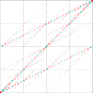
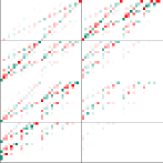
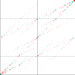
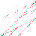
The top panel of figure 4 shows the ground state of equation 3, while the bottom row shows the first three excited states, which constitute a spin-1 triplet.

Figure 4: Top: Ground state of the 1D spin-$1/2$ AF Heisenberg model with PBC for 12 spins; Bottom: the lowest energy excitations, which make up a triplet. White means zero probability, color intensity reflects the modulus of the wavefunction amplitude, while color hue marks the phase.

Let us focus on the ground state (figure 4, top panel). The most salient feature is its intense diagonal line, joining the two Néel states, which get maximal weight. The states conforming that diagonal are all made up of pairs $01$ and $10$, in any order. This main diagonal is the depiction of a set of pairwise singlet bonds: $(1,2)(3,4)\cdots(N-1,N)$.

There is another interesting feature in this image. The two parallel diagonal lines with slope $1/2$ have the same intensity as the main diagonal. What is their origin? A clue can be obtained when we depict the GS of the Heisenberg model with open boundary conditions (see figure 5). It is apparent that these secondary lines have almost disappeared. In order to finally clarify the nature of these secondary lines, let us consider ${\cal R}$, the right-shift translation operator (with periodic boundary conditions). If ${\cal R}$ acts on the states composing the main diagonal, the result is the two secondary diagonals, and viceversa, as it can be seen in figure 6. It is now straightforward to provide a physical interpretation: the secondary diagonals depict the other possible set of pairwise singlet bonds: $(2,3)(4,5)\cdots(N,1)$. When periodic boundary conditions are employed, both structures are equally important, but not under open ones.

c

Figure 5: Ground state of the 1D spin-$1/2$ AF Heisenberg model with open boundary conditions and $N=12$ spins. Notice that, as opposed to the case of figure 4, the secondary diagonals have almost vanished.

Figure 6: The two diagonal structures which make up the Heisenberg ground state are related through a right-shift translation operator ${\cal R}$. If $(i,j)$ denotes a singlet bond, on the left we have $(1,2)(3,4)\cdots(N-1,N)$, and $(2,3)(4,5)\cdots(N,1)$ on the right.

The slope $1/2$ of those secondary diagonals can be understood as follows. According to equation 2, acting with the right-shift translation operator ${\cal R}$ on a state given by bits $\{X_{1}Y_{1}X_{2}Y_{2}\cdots X_{n}Y_{n}\}$ we obtain $\{Y_{n}X_{1}Y_{1}X_{2}\cdots Y_{n-1}X_{n}\}$. Thus, ${\cal R}$ maps the point $(x,y)$ into a point very close to $((y+Y_{n})/2,x)$. Consequently, the image of the $x=y$ line is approximately $x=(y+Y_{n})/2$, i.e.: the two secondary lines. A second application of the right-shift operator ${\cal R}$ on these two secondary lines returns the original main diagonal. Of course, the same effect is obtained with a left-shift.

3.2 Next-nearest-neighbour Heisenberg: Marshall rule and Frustration

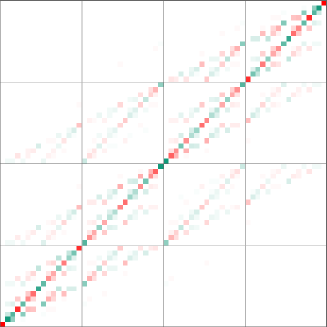
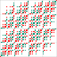
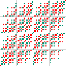
Still there is one more interesting feature of the image of the ground state of the Heisenberg Hamiltonian, 4. According to Marshall’s rule [15], the sign of each wavefunction component of the ground state of the Heisenberg AF model in a bipartite lattice (split into sublattices $A$ and $B$) can be given as $(-1)^{N_{A}}$, where $N_{A}$ is the number of up-spins in sublattice $A$. In our case, a 1D lattice with PBC, the two sublattices are just the odd and even sites. It is not hard to recognize that, if we select the odd sites to make up sublattice $A$, then the sign rule tells us that all states in the same horizontal line must have the same sign. But, on the other hand, if sublattice $A$ is made up with the even sites, then the rule tells us that all states in the same vertical line will have the same sign. Both conditions can be fulfilled, both in the PBC and the OBC figures, 4 and 5.

Marshall sign rule can not be applied if the system presents frustration, i.e.: when the Hamiltonian couples spins in the same sublattice $A$ or $B$. Let us consider the next-nearest-neighbour AF Heisenberg Hamiltonian (also known as $J_{1}J_{2}$ model):

$$H=J_{1}\sum_{i=1}^{N}{\vec{S}}_{i}\cdot{\vec{S}}_{i+1}+J_{2}\sum_{i=1}^{N}{\vec{S}}_{i}\cdot{\vec{S}}_{i+2}$$ (4)

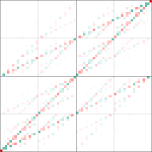
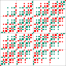
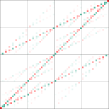
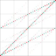
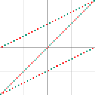
where $J_{1}=1$ and $J_{2}>0$. Then, as $J_{2}$ increases, the system undergoes a quantum phase transition (QPT) at around $J_{2}\approx 0.24$. Figure 7 shows how the sign-structure is destroyed slowly as $J_{2}$ is increased from $J_{2}=0$ to $J_{2}=1/2$. The point $J_{2}=1/2$ is special, since the ground state is then exactly known: the Majumdar-Ghosh point. Its rather simple structure is apparent in figure 8.

Figure 7: Destruction of the sign pattern given by Marshall rule as $J_{2}$ increases for the ground state of the Hamiltonian given in eq. 4., with $N=12$ qubits and PBC. From top to bottom, the values of $J_{2}$ are $J_{2}=0$, $0.2$ and $0.3$. The left column shows the full image. The right one only depicts the phases of the non-zero amplitude values.

Figure 8: Majumdar-Ghosh state, ground state of the Hamiltonian in equation 4 with $N=12$ qubits and PBC for $J_{2}=0.5$.

3.3 Product States

Let us now consider the simplest possible quantum many-body wavefunction: a translationally invariant product state, defined as

$$\left|\Psi\right>=\left(\alpha\left|0\right>+\beta\left|1\right>\right)^{N}$$ (5)

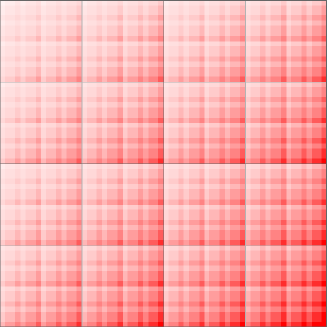
Factorizability is a very strong property, which shows itself in a very appealing way in our plots. Figure 9 shows such a product state in the $\sigma_{z}$ basis. Physically, factorizability implies that measurements performed on any qubit should have no influence on the remaining ones. Concretely, we can measure $\sigma_{z}$ on the first two qubits. If the result is $00$, the wavefunction-plot which describes the rest of the system will be (a normalized and rescaled version of) the upper-left quadrant of the plot. Correspondingly, if the results are $01$, $10$ or $11$, the wavefunction-plot will be just a (normalized and rescaled version of) other quadrant. Thus, factorizability implies that all four quadrants are equal (modulo a normalization factor). This line of thought can be extended to the set of the first $2k$ qubits, thus showing that if we split the plot into a $2^{k}\times 2^{k}$ array of sub-images, they should all coincide, modulo a normalization factor. This gives the characteristic look to the plots of product states. We will return to this topic in section 6, when we discuss entanglement.

Figure 9: Product state following equation 5 with $\beta/\alpha=1.3$.

3.4 Dicke states

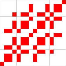
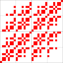
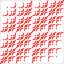
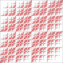
Another interesting example is provided by the so-called Dicke states [16]. Those are defined as the linear combination, with equal weights, of all tensor basis states with the same number $n_{e}$ of $1$’s in their decomposition. In our examples, we will focus on the half-filling case, $n_{e}=N/2$. In fermionic language, they constitute the ground state of a free-fermion model with homogeneous diffusion on a complete graph at half-filling, and in spin-$1/2$ language it is the $S_{z}=0$ component of the maximal spin multiplet. Figure 10 shows the pattern obtained for different lattice sizes. It is apparent how a fractal develops. Their similarity to the right column of figure 7 is, of course, not casual: the ground states of the Heisenberg-like models have global magnetization zero, which make them similar to half-filling Dicke states.

Figure 10: Half-filling Dicke states for $N=8$, $10$, $12$ and $14$ qubits. Notice how the fractal structure develops.

3.5 Ising model in a transverse field: Criticality

As a different relevant example, let us consider the spin-$1/2$ AF Ising model in a transverse field (ITF), in a 1D chain with PBC:

$$H=\sum_{i=1}^{N}\sigma^{z}_{i}\sigma^{z}_{i+1}-\Gamma\sum_{i=1}^{N}\sigma^{x}_{i}$$ (6)

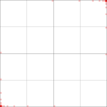
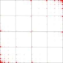
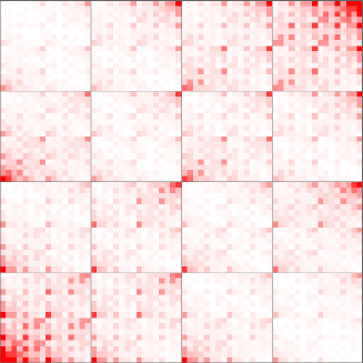
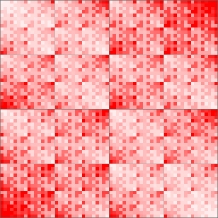
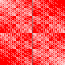
For $\Gamma=1$, the system presents a quantum phase transition (QPT). Figure 11 shows the plots obtained from the GS for different values of $\Gamma$. For $\Gamma\to 0$, the ground state consists only of the two Néel states. As $\Gamma$ increases (first two top panels), the points which come up first correspond to a single defect, at all possible positions in the lattice. The non-zero probability amplitudes extend further away from the original corner states as $\Gamma$ approaches criticality, and at that point $\Gamma_{c}=1$, the non-zero values have extended through the whole image, albeit quite inhomogeneously. From that point, increasing $\Gamma$ makes the image more and more homogeneous. For $\Gamma\to\infty$, the ground state would consist of all spins pointing in the $X$-direction, and this implies that the wavefunction components will all take the same value.

Figure 11: Ground states of the AF ITF Hamiltonian with $N=12$ qubits and PBC. Values of the transverse field are: (top) $\Gamma=0.2$ and $0.6$, (central) $\Gamma=\Gamma_{c}=1$, (bottom) $\Gamma=1.4$ and $1.8$.

3.6 Infinite-range Hamiltonians

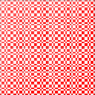
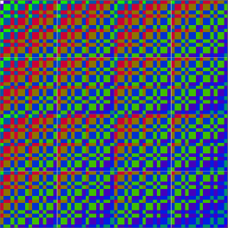
And let us finish this section by considering infinite-range Hamiltonians, i.e.: those in which all spins are linked to all others. They can be thought of as infinite-dimension or mean-field systems. Those Hamiltonians commute with the full set of generators of the permutation group. Therefore, their ground states are often invariant under it. Compared to translation invariance, this symmetry group is so large ($N!$ elements vs. $N$) that it leaves very little freedom: a fully permutation-invariant wavefunction of $N$ qubits is characterized by just $N+1$ independent components, one per global magnetization sector. Thus, permutation-invariant wavefunctions have a clear visual fingerprint.

Figure 12 (left) shows the GS of the infinite-range AF ITF Hamiltonian for $\Gamma=1$ and $N=12$ qubits, illustrating this high degree of symmetry. The right part of the figure shows a random permutation-invariant state. It is not a coincidence that it reminds so strongly of the Dicke states, since each magnetization sector shares the same color. The infinite-range Heisenberg Hamiltonian ground state is not shown because it is strongly degenerate, so invariance under the permutation group remains only as a property of the full subspace.

Figure 12: Left: Ground state of the AF infinite-range ITF model for $\Gamma=1$ with $N=12$ qubits. Right: a random permutation-invariant state, also with $N=12$ qubits.

4 Other Plotting Schemes

4.1 General Formulation

The previous procedure can be generalized in the following way. Let $D$ be any domain in ${\mathbb{R}}^{d}$, which can be partitioned into $m$ congruent subdomains $S_{i}D$, with $i\in\{0,\cdots,m-1\}$, all of them similar to $D$. In our current example, $D=[0,1]\times[0,1]$, the unit square, which is divided into $m=4$ smaller squares, which we denote by $S_{0}D$ (upper-left), $S_{1}D$ (upper-right), $S_{2}D$ (lower-left) and $S_{3}D$ (lower-right).

The action of operators $S_{i}$ can be iterated. Thus, $S_{1}S_{3}D$ denotes the upper-right quadrant of the lower-right quadrant of the original square. We can define a geometrical index as a sequence of integers $I_{G}\equiv\{i_{k}\}_{k=1}^{n}$, with $i_{k}\in\{0\cdots m-1\}$. Each geometrical index denotes a (small) domain $S_{i_{1}}\cdots S_{i_{n}}D$, similar to the original one. In our example, a tiny square. We can, thus, define a mapping ${\cal S}$ which converts geometrical indices into regions of ${\mathbb{R}}^{d}$ which are similar to $D$: ${\cal S}(I_{G})\equiv S_{i_{1}}\cdots S_{i_{n}}D$.

Now let us focus on the tensor-product structure of the quantum Hilbert space. Each state is characterized by a quantum index, i.e.: a set of $N$ indices taken from certain discrete finite set: $I_{Q}\in\Sigma^{N}$. In our case, $\Sigma=\{0,1\}$. In the case of spin-1 systems, $\Sigma=\{-1,0,1\}$ or, more simply, $\Sigma=\{-,0,+\}$.

The last piece of the scheme is a function ${\cal M}$ mapping quantum into geometrical indices, ${\cal M}:\Sigma^{N}\mapsto\{0,\cdots,m-1\}^{n}$, such that $I_{G}={\cal M}(I_{Q})$. In our case, this function groups the quantum indices in pairs, and combines each pair into a single geometrical index with the simple binary mapping: $00\to 0$, $01\to 1$, $10\to 2$, $11\to 3$. It should be noted that $n=N/2$. This mapping should be bijective, so as not to lose information.

Now, the full wavefunction plotting scheme ${\cal K}$ is defined by providing the original region, $D$, the set of similarity transformations, $\{S_{i}\}$, $i\in\{0,\cdots,m-1\}$ and the indices mapping function ${\cal M}$. Thus, ${\cal K}(I_{Q})$ will denote the region in ${\mathbb{R}}^{d}$ obtained by applying ${\cal S}$ to the geometrical index associated to $I_{Q}$, i.e.: ${\cal K}(I_{Q})={\cal S}({\cal M}(I_{Q}))$. Those cells make up a partition of $D$. It is easy to prove the essential properties:

$$\cup_{Q\in\Sigma^{N}}{\cal K}(I_{Q})=D$$

$${\cal K}(I_{Q})\cap{\cal K}(I_{Q}^{\prime})=\emptyset\quad\Longleftrightarrow\quad I_{Q}\neq I_{Q}^{\prime}$$ (7)

Thus, for every $x\in D$, there exists a single $I_{Q}\in\Sigma^{N}$ such that $x\in{\cal K}(I_{Q})$. This property ensures that we have can pull-back wavefunctions, i.e.: functions $\psi:\Sigma^{N}\mapsto{\mathbb{C}}$, into complex-valued functions on $D$, ${\cal K}(\psi):D\mapsto{\mathbb{C}}$.

So, can we devise other possible plotting schemes? Will they make different properties apparent? We will approach those questions in the rest of this section.

4.2 1D plot

The simplest possible plotting scheme can be realized in 1D for qubits. Let $D$ be the $[0,1]$ segment, split every time into two halves: $S_{0}$ selects the left part, and $S_{1}$ the right one. Now, the resulting ${\cal K}$ mapping is equivalent to a binary lexicographical ordering of the wavefunction components. More explicitly: divide the domain $[0,1]$ into $2^{n}$ equal cells, index them from $0$ to $2^{n}-1$ and attach to each of them the wavefunction component with the same associated index.

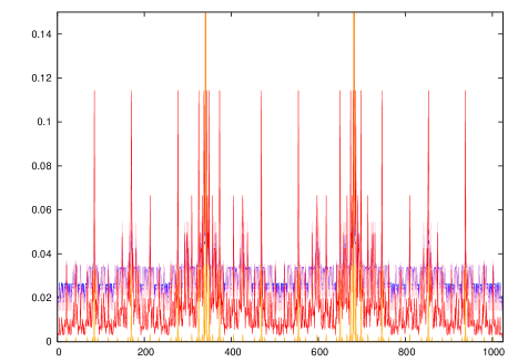
Figure 13 shows plots (1D) of the ground state of the antiferromagnetic ITF model, equation 6, for several values of $\Gamma$. This plotting scheme is, evidently, much less appealing than the bidimensional ones. On the other hand, its simplicity is helpful when attempting to clarify some of the features, e.g. the Fourier analysis made in section 5.

Figure 13: 1D representation of the AF ITF ground state with $N=10$ qubits and PBC for a few values of $\Gamma$.

4.3 Spin-1 plots: AKLT states

As we have already stated, the quantum indices can be built upon any local set of quantum numbers. For a set of spin-1 particles, the choice is $\Sigma=\{-1,0,1\}$ or, more simply, $\Sigma=\{-,0,+\}$. If we start with the same domain, $D=[0,1]^{2}$, the natural decomposition is into $3\times 3$ subdomains, as shown in the following (cartesian product) scheme:

$$\begin{array}[]{|c|c|c|}\hline\cr--&-0&++\\ \hline\cr 0-&00&0+\\ \hline\cr+-&+0&++\\ \hline\cr\end{array}$$ (8)

Of course, this is not the only possible mapping. With this one, we have chosen to show the structure of the Affleck-Kenedy-Lieb-Tasaki (AKLT) state [17]. It is the ground state of the following Hamiltonian:

$$H=\sum_{i=1}^{N}{\vec{S}}_{i}\cdot{\vec{S}}_{i+1}+{1\over 3}({\vec{S}}_{i}\cdot{\vec{S}}_{i+1})^{2}$$ (9)

This state is an example of valence bond solid (VBS), and has attracted considerable attention because of its relation to the Haldane conjecture [18], its non-local order parameter [19] and as a source of inspiration of tensor-network states [20].

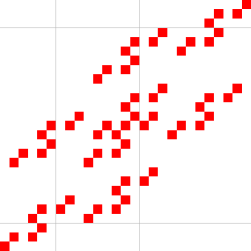
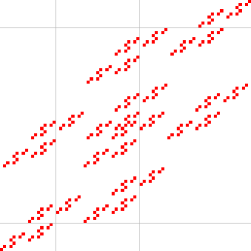
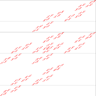
The result can be seen in figure 14 where, for better visualization, we have marked only the non-zero components of the wavefunction. Notice the strong self-similarity appearance.

Figure 14: Ground state of the AKLT spin-1 Hamiltonian, for $N=6$, $8$ (top) and $10$ (bottom) spins. Notice how the fractal structure develops.

4.4 Alternative Square Plot

Restricting ourselves to qubits and ${\cal D}=[0,1]^{2}$, it is still possible to have another inequivalent plotting scheme, by changing the assignments:

$$\begin{array}[]{ccc}00\to\hbox{Upper left}&01\to\hbox{Upper right}\\ 11\to\hbox{Lower left}&10\to\hbox{Lower right}\\ \end{array}$$ (10)

In this new plotting scheme the two left corners (top and bottom) represent the FM states, and the right corners the Néel states.

It can be shown that these two are the only possible inequivalent plotting schemes for qubits on $[0,1]^{2}$. The reason is the following. There are $4!=24$ possible associations between $\{00,01,10,11\}$ and the four quadrants. The group of symmetries contains three rotations, two reflections on the horizontal and vertical axes and two reflections on the two diagonals, i.e.: 12 different elements. This leaves only $4!/12=2$ inequivalent choices.

As an example, figure 15 (left) shows the ground state of the critical ($\Gamma=1$) ITF model with $N=12$ qubits (eq. 6). It is therefore, an alternative pictorial representation of figure 11. Figure 15 (right) shows the ground state of the Heisenberg model with $N=12$ qubits, in the new plotting scheme. The Néel states are now situated in the lower and upper right corners. Therefore, the main diagonal line, hallmark of the spin-liquid structure, lies now in the rightmost vertical line. The secondary diagonals, on the other hand, are now dispersed, in a Sierpiński-like structure.

Figure 15: Alternative 2D representations, following equation 10, with $N=12$ qubits and PBC. Left: Ground state of the critical AF ITF model. Right: Ground state of the Heisenberg model. Compare, respectively, to figures 11 (central) and 4.

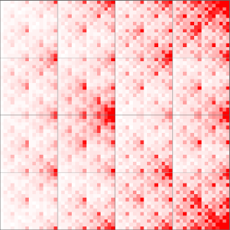
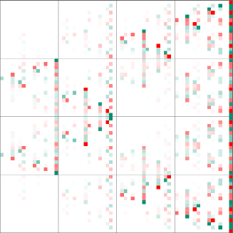
It is apparent that figure 15 (bottom) is smoother than its counterpart, figure 11 (central). All possible plotting schemes are equally valid, in principle, just as a polar and a cartesian representation of the same function are. Can we provide some sense of plotting quality? Perhaps: a smoother plot suggests that the neighbourhood structure of the original wavefunction is respected more properly by the plotting scheme.

4.5 Triangular Scheme

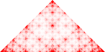
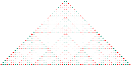
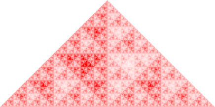
It is possible to design a 2D plotting scheme of qubits which does not require grouping the quantum indices in pairs. Let $D$ be a rectangular isosceles triangle of unit side, with vertices at $(-1,0)$, $(0,1)$ and $(1,0)$. It can be split into two similar triangles, of side $1/\sqrt{2}$. Let $S_{0}$ and $S_{1}$ be the operators which select the left and right triangles (as seen when the right-angle vertex is up). Figure 16 shows how such a representation maps bits into cells. Within this scheme the Néel states go towards the left and right bottom corners. The FM states correspond to two points near the center, symmetrically placed with respect to the height. In the thermodynamical limit, these FM points can be obtained summing a geometrical series: $(\pm 1/5,2/5)$.

Figure 16: Plotting scheme using rectangular triangles. Top and center: first two iterations. Bottom: First four iterations (dashed lines). The two Néel states of the fifth iteration are the bottom left and right filled corner triangles. The two FM states correspond to the symmetrically placed filled triangles near the center.

Figure 17 depicts the ground states of the critical ITF and the Heisenberg model, and a product state. Notice that the diagonal lines in the original representation for the Heisenberg GS have mapped now to the perimeter of the triangle. The main diagonal is the hypotenuse, the two secondary diagonals are the other two sides. The remaining structure, which was not quite clean in the original representation, comes here as a Sierpiński-like structure.

Figure 17: Triangular representations of many-body wavefunctions. Top: GS of the AF-ITF model with $N=12$ qubits and PBC. Center: GS of the Heisenberg model with $N=12$ qubits and PBC. Bottom: product state with $N=12$.

4.6 More Exotic Plotting Schemes

We will now propose other plotting schemes in order to show the versatility of the procedure.

In the case of spin-1 systems, the only alternative that we have found in order to make the quantum and the geometrical indices coincide is to work on a Sierpiński triangle. The original domain is, this way, naturally split into three similar domains: $S_{-}D$, $S_{0}D$ and $S_{+}D$. Nonetheless, it has the disadvantage that the domain is not simply connected.

Even more exotic plotting schemes are conceivable. Let $A_{0}$ be a regular hexagon. Now proceed to build $A_{1}$ as the union of $A_{0}$ and six congruent hexagons built upon its sides. Repeating the scheme, and rescaling at each step, we reach a fixed point: $A_{\infty}$, with the following property: it can be split naturally into $7$ similar cells of exactly the same shape [21].

5 Self-similarity of the wavefunction plots

The plotting schemes described in the present article are evidently self-similar. It is obvious that the first qubit determines the largest-scale properties of the plot, and subsequent qubits determine lower scales properties. The question that we will address is: how does this self-similarity of the scheme map into fractal or self-similar properties of the wavefunction plots?

5.1 Translation-invariance and self-similarity

Let ${\cal R}$ be the cyclic right-translation shift. A wavefunction has translational symmetry if, for any quantum index $I_{Q}$, $|\psi(I_{Q})|=|\psi({\cal R}(I_{Q}))|$. Does this symmetry bear any visual consequences in the wavefunction plots?

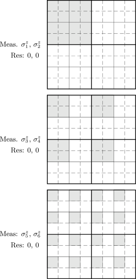
In a translationally invariant system, a measurement performed on the first two qubits and another performed on the last two should have the same effects. Let us focus on a given possible outcome of the measurement, e.g.: $00$. Now, the wavefunctions describing the rest of the system should coincide. If the measured qubits are the first two, the new wavefunction-plot is obtained by selecting the upper-left quadrant of the original plot. On the other hand, if the measurement has been done on the last two qubits, we should decimate: group the plot pixels into $2\times 2$ blocks, and select the upper-left pixel out of each block. Both wavefunctions should coincide, as a result of translation-invariance.

So, plots of translation-invariant wavefunctions display self-similarity in the following sense. Divide the plot into a matrix of $2^{k}\times 2^{k}$ sub-plots ($k\in\{0,\cdots n-1\}$) and do a further division of each sub-plot into $2\times 2$ quadrants. Selecting the same quadrant from each sub-plot and rebuilding a full image will yield the same result, for all possible values of $k$. Figure 18 illustrates the criterion.

Figure 18: Illustrating translation invariance properties in a qubistic plot. All three plots represent the qubistic representation of a $N=6$ wavefunction. Assume we measure $\sigma^{z}$ on qubits 1 and 2, and the results are 0 and 0. Then, after the measurement, the wavefunction-plot will be given by the marked cells of the top plot. The central and bottom plots are equivalent, but with measurements performed on qubits $\{3,4\}$ and $\{5,6\}$ respectively. If the wavefunction is translation-invariant, all three resulting wavefunction-plots should be exactly equal.

5.2 Measures of scale invariance

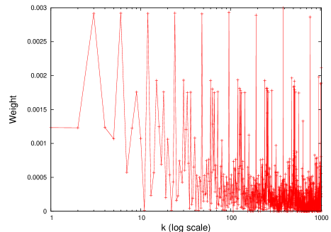
Scaling invariance of the wavefunction plots should also be visible in the Fourier transform. In effect, figure 19 shows the transform of a 1D-plot of an AF ITF Hamiltonian (eq. 6) with $N=10$ qubits and PBC. The momenta are displayed in logarithmic scale, and we can spot a clear periodic structure. Evidently, exact log-periodicity is impossible to achieve since each period contains a larger number of degrees of freedom than the preceding one. This feature is visible for a wide range of transverse fields, i.e.: it is not linked to criticality.

Figure 19: Fourier transform of the ground state of the 1D plot of the critical ITF model, with $N=10$ qubits and PBC, for $\Gamma=0.6$.

Another interesting indicator of self-similarity is provided by the Rényi fractal dimensions [Halsey.86]. Let us consider the probability distribution associated to a wavefunction plot (taking the modulus squared), $P_{N}=\{p_{N,i}\}$ for $N$ qubits. We can compute the Rényi entropy of order $q$, i.e.:

$$R_{q}(P^{(N)})\equiv{1\over 1-q}\log\left(\sum_{i}p_{N,i}^{q}\right)$$ (11)

Now we define the Rényi dimensions by:

$$d_{q}\equiv\lim_{N\to\infty}{R_{q}(P_{N})\over\log\left(b^{N/2}\right)}$$ (12)

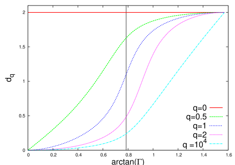
where $b$ is $2$ for qubits or $3$ for spin-1. With this notation, $d_{0}$, $d_{1}$ and $d_{2}$ are, respectively, the support, information and correlation dimensions of the fractal. The full set of $d_{q}$ provide the same information as the multifractal spectrum.

Figure 20 shows a few Rényi dimensions for an AF ITF model as a function of $\Gamma$. In our case, the support dimension $d_{0}$ is always $2$, since all probability values are non-zero. All the other dimensions interpolate between $0$ (for $\Gamma\to 0$) and $2$ ($\Gamma\to\infty$). The information dimension, $d_{1}$ seems to capture most accurately the physical properties of the model, since its growth rate is maximal at the critical point.

Figure 20: Rényi fractal dimensions (equation 12) of the wavefunction plot of the ground state of the AF ITF model with PBC. Notice that the $X$-axis is labeled with $\arctan(\Gamma)$ in order to highlight the symmetry. The vertical bar shows the critical case, $\Gamma_{c}=1$. Computations are carried out for $N=10$ qubits, but the results are quite independent of the system size.

It is an interesting exercise to prove that, for the AKLT state shown in figure 14, all Rényi dimensions with $q>0$ are equal to $\log(4)/\log(3)\approx 1.26$.

6 Visualization of entanglement

One of the most intriguing features of quantum many-body systems is entanglement. A system is entangled if measurement on one of its parts affects the results of subsequent measurements on others, even if they are well separated. Einstein himself described this phenomenon as “spukhafte Fernwirkung” (spooky action at a distance) [22]. It is considered as a resource for quantum computation and communication [23], as well as providing very useful insight regarding quantum phase transitions [24].

6.1 Visual estimate of entanglement

Is entanglement visualizable from our wavefunction plots? Yes. Summarizing the results of this section we may say that entanglement shows as image complexity. Let us consider all quadrants of level-$k$ within the plot, normalized. If there are only $p$ different quadrants, then the entanglement entropy is $\leq\log(p)$. Concretely, if all level-$k$ quadrants are equal, the system is factorizable.

In section 3.3 we discussed product states, i.e.: systems without entanglement. Let us recall the conclusions exposed in that section. If the first two qubits are disentangled from the rest of the system, measurements made upon them should not have influence on the rest. Therefore: all four quadrants of the plot are equal (modulo normalization). If all the qubits are disentangled (at least by pairs), then the result is extended: if the plot is split into a $2^{k}\times 2^{k}$ matrix of subimages, for all $k$, all the sub-images are equal (modulo normalization). This result can be expressed in a more concise way: the plot of a product state is trivially self-similar. Every quadrant, of every size, is the same as any other, after proper normalization.

What happens if the system is entangled? Let us now consider a generic wavefunction, $\left|\Psi\right>$, and split the system into a left and a right parts, $L$ and $R$. The left part will correspond to qubits 1 to $2k$ and the right part to qubits $2k+1$ to $N$, for any $k$. We can always perform a Schmidt decomposition:

$$\left|\Psi\right>=\sum_{i=1}^{m}\lambda_{i}\left|\psi^{L}_{i}\right>\otimes\left|\psi^{R}_{i}\right>$$ (13)

where the orthonormal sets $\{\left|\psi^{L}_{i}\right>\}$ and $\{\left|\psi^{R}_{i}\right>\}$ are called the left and right-states, and characterize the physics of each part, $\lambda_{i}$ are called the Schmidt coefficients and $m$ is the Schmidt rank, which is a measure of entanglement. If $m=1$, the state is factorizable. A state with Schmidt rank $m$ can not have entanglement entropy larger than $\log(m)$.

The left part corresponds to the larger scales, and the right part to the smaller ones. Let us make this statement concrete.

Consider the Hilbert space for the left part, and let $\{\left|x\right>\}$ be the basis of tensor states for it. E.g.: if $k=1$, the left part has two qubits and the states $\{\left|x\right>\}$ are $\left|00\right>$, $\left|01\right>$, $\left|10\right>$ and $\left|11\right>$. Now we will consider what are their geometric counterparts in the wavefunction plot. Within the original 2D plotting scheme, qubits 1 to $2k$ correspond to the first $k$ quadrant divisions. Let us divide the original plotting square into a matrix of $2^{k}\times 2^{k}$ quadrants. Each tensor state $\left|x\right>$ can be attached to one of these quadrants, which we will denote simply by $x$.

The left-states, $\left|\psi^{L}_{i}\right>$ can be expressed as

$$\left|\psi^{L}_{i}\right>=\sum_{x}\psi^{L}_{ix}\left|x\right>$$ (14)

Now, let us focus on the right part. Each right-state, $\left|\psi^{R}_{i}\right>$ can be plotted inside a level-$k$ quadrant using the standard representation. Let us call the corresponding plot $R_{j}$.

What is the actual image, for the full wavefunction plot, on the $x$-th quadrant? Inserting equation 14 into the Schmidt decomposition 13 we can see that it is given by the expression

$$C(x)=\sum_{i=1}^{m}\lambda_{i}\psi^{L}_{ix}R_{i}$$ (15)

The conclusion is that, for each level-$k$ quadrant the plot is a linear combination of the $m$ right-state plots, with weights given by the the left-states components and the Schmidt coefficients.

Therefore, level-$k$ quadrants within the final plot are built upon only $m$ fundamental images, or building bricks, which are the plots of the right-states. In other terms: the Schmidt rank $m$ for a given left-right partition coincides with the effective dimension of the subspace spanned by all images in level-$k$ quadrants. This statement provides a way to give a coarse estimate the entanglement of the wavefunction: if, at level-$k$, the number of different quadrants is $p$, then the block of the first $2k$ qubits has a Schmidt rank of $m\leq p$, and the entanglement entropy is $S\leq\log(p)$. As a corollary, if all quadrants are exactly the same, then $m=1$ and $S=0$, the system is factorizable, as we already stated.

The logic behind the estimate is to find the number of different building blocks at each scale. If we want to be precise, the Schmidt rank is given by the dimension of the subspace spanned by all quadrant images at a certain level, but this value is much more difficult to estimate visually.

Let us apply the estimate in a set of simple cases, with $N=4$ qubits (i.e.: only two levels). Figure 21 shows the qubistic plots for a set of states similar to those of figure 3. Since entanglement is invariant under local changes of basis, we also show the qubistic plot in the basis of eigenstates of $\sigma^{x}$. Both plots provide a similar estimate, which is compared in each case with the exact value. (A) The state $\left|0000\right>$ is factorizable, which can be seen in both plots. In the $\sigma^{z}$ plot, only one of the sub-images is non-zero. In the $\sigma^{x}$ picture, all four sub-images are the same, modulo a sign. (B) The GHZ is not factorizable. In both basis can be seen that the number of different sub-images is 2. (C) corresponds to the W state, which is a bit more complex. In the $\sigma^{z}$ basis it is evident that the number of different sub-images is 2, which corresponds to the Schmidt rank. In the $\sigma^{x}$ basis, the visual estimate gives 3 different sub-images. Our prediction is still valid, since the estimate only provides an upper bound. The reason for the error is that the 3 sub-images are not linearly independent. This example serve as a warning: some basis may provide clearer visual estimates than others. (D) Is the Dicke state at half-filling. In this case the visual estimate coincides for both basis, 3 different sub-images. But do not have the same weight, and the von Neumann entropy is smaller than $\log(3)$. (E) The $\left|0000\right>+\left|1111\right>-\left|1010\right>-\left|0101\right>$ state has four different sub-images in both basis, and achieves maximal Schmidt rank and entanglement entropy.

	(A)	(B)	(C)	(D)	(E)
$\sigma^{z}$ basis
$\sigma^{x}$ basis
Schmidt rank:	1	2	2	3	4
Von Neumann entropy:	$0$	$\log 2=1$	$\log 2=1$	$\log 3-\frac{1}{3}$	$\log 4=2$
				$\approx 1.25$

Figure 21: Visual estimates of entanglement using qubistic plots for some relevant states of $N=4$ qubits. The first row shows the usual qubistic plots in the $\sigma^{z}$ basis. The second row, on the other hand, depicts the plots using the $\sigma^{x}$ basis. Since entanglement is invariant under local changes of basis, the visual estimate of entanglement should not change. The third row provides the Schmidt rank in all cases for the separation between the first and second pairs of qubits, and the fourth row contains the von Neumann entropy (logarithms are always with basis 2). The states correspond to the columns: A.- $\left|0000\right>$; B.- GHZ state; C.- W state; D.- Dicke state at half filling; E.- $\left|0000\right>+\left|1111\right>-\left|1010\right>-\left|0101\right>$.

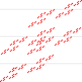
The strategy can be applied to the AKLT state, depicted in figure 14. At any splitting level the exact number of different images is always 5. But, as the number of sites increases, some of these images become more and more alike, until only 3 of them are distinguishable. Figure 22 shows the sub-image pattern more clearly. See, for example, the $-+$ and $0+$ quadrants of the plots in figure 14: their differences are easy to spot for $N=6$, but almost unnoticed for $N=10$. This implies that the Schmidt rank is always $\leq 3$, providing the estimate $S\leq\log(3)$, independent of the depth level, which is exactly the actual value in the thermodynamic limit [25].

0 A B A C B A B 0

Figure 22: AKLT qubistic plot for $N=8$ spins and the associated sub-image pattern: boxes with the same letter contain (very approximately) the same sub-image.

On the other hand, taking the half-filling Dicke states of figure 10, it is evident that, at every magnification level, the number of different subimages increases by two. Thus, $S(k)\leq\log(2k+1)$ in terms of levels, or $S(l)\leq\log(l+1)$ for qubits, if $l\leq N/2$. This bound is found to be fulfilled by the numerical calculations shown in figure 23.

Figure 23: Entanglement entropy of a block of $l$ sites in a half-filling Dicke state of $L=10$, $12$ and $14$ sites, compared to the upper bound obtained from the qubistic plot, which is $S(l)\leq\log(l+1)$.

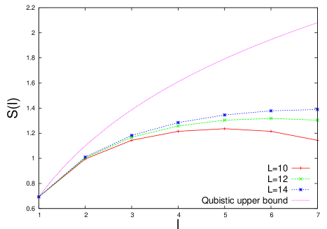
The reason for the difference between the estimate and the actual values of entanglement in fig. 23 is twofold. First, the number of different level-$l$ quadrants is, in general terms, a very poor way to estimate the dimension of the subspace spanned by them. Second, the value estimated this way is just the Schmidt rank, whose logarithm is just an upper bound to the actual entanglement entropy. Both problems can be handled within the more comprehensive framework, described in the next section.

6.2 Entanglement and the cross-correlation matrix

Given a wavefunction plot and a level $k$, let us divide the full region into a grid of $2^{k}\times 2^{k}$ sub-plot. Moreover, let $x$ be an index running through all such sub-plots and $C(x)$ be the actual image displayed in it, as in equation 15. Now we define a cross-correlation matrix for the plot image, $R(x,x^{\prime})$, as

$$R(x,x^{\prime})=\langle C(x)|C(x^{\prime})\rangle$$ (16)

This cross-correlation matrix bears full information about entanglement of the first $2k$ qubits within the wavefunction, as we proceed now to show.

According to equation 15, the image on quadrant $x$ is given by a linear combination of the right-states. Using the orthogonality property assumed for them we obtain

$$R(x,x^{\prime})= \sum_{i,j=1}^{m}\left<\psi^{R}_{i}\right|\psi^{L*}_{ix}\lambda_{i}\lambda_{j}\psi^{L}_{jx^{\prime}}\left|\psi^{R}_{j}\right>$$

$$= \sum_{i=1}^{m}\lambda_{i}^{2}\psi^{L*}_{ix}\psi^{L}_{ix^{\prime}}$$ (17)

Thus, we recognize that $R(x,x^{\prime})$ is just the density matrix for the left part. In other terms:

$$R(x,x^{\prime})=\rho^{L}_{xx^{\prime}}$$ (18)

Therefore, the cross-correlation matrix of the wavefunction plot holds full information related to entanglement.

For example, for a product state, all subimages are equivalent modulo normalization. Thus, we can assume that

$$R_{F}(x,x^{\prime})=N(x)\cdot N(x^{\prime})$$ (19)

with $N(x)=\langle C(x)|C(x)\rangle^{1/2}$ is the norm for each subimage. Obviously, $\sum_{x}N^{2}(x)=1$ and, thus, the matrix $R_{F}$ is just a projector on a line. Its spectrum is, in decreasing order, $\sigma(R_{F})=\{1,0,\cdots,0\}$. Therefore, its entanglement entropy is zero.

7 Frame representation

In this last section we describe a rather different approach to the problem of providing a graphical representation of a quantum many-body system, but still self-similar by design. Instead of plotting wavefunction amplitudes, or probabilities, we can plot the expectation values of a bidimensional array of operators, chosen in such a way that the full information contained in the wavefunction is preserved. This is called a frame representation of the quantum state [26]. According to Wootters and coworkers [12], the final representation may correspond to a discrete analogue of a Wigner function [27], with very interesting properties in order to characterize non-classicality, such as its negativity [28].

Let us consider a system of $n$ qubits, described by a certain density matrix $\rho$. Now, let us consider the unit square $[0,1]\times[0,1]$ and any two numbers, $x$ and $y$, characterized by their binary expansion: $x=0.X_{1}X_{2}\cdots X_{n}$, $y=0.Y_{1}Y_{2}\cdots Y_{n}$. The value attached to the point $(x,y)$ in the plot will be given by the expectation value in $\rho$ of the operator $A(x,y)$:

$$f(x,y)=\tr\left[\rho A(x,y)\right]$$ (20)

where $A(x,y)$ is given by:

$$A(x,y) =\bigotimes_{k=1}^{n}(-i)^{X_{k}Y_{k}}\left(\sigma_{k}^{x}\right)^{X_{k}}\left(\sigma_{k}^{y}\right)^{Y_{k}}$$ (21)

$$=\bigotimes_{k=1}^{n}\sigma_{k}^{X_{k}+2Y_{k}}.$$ (22)

In other words, we plot the expected value of every combination of tensor products of $\{\sigma^{0}\equiv I,\ \sigma^{1}\equiv\sigma^{x},\ \sigma^{2}\equiv\sigma^{y},\ \sigma^{3}\equiv\sigma^{z}\}$. In particular, on the $y=0$ line we get uniquely correlations in $\sigma_{x}$; on $x=0$, those in $\sigma_{y}$, and on $x=y$ those corresponding to $\sigma_{z}$. Such representation is unique for every density matrix, and can be reverted as follows:

$$\rho=\sum_{x,y}\frac{1}{2^{n}}f(x,y)A(x,y).$$ (23)

In order to attain some intuition about the representation, figure 24 illustrates it for one and two qubits. At each cell, we depict the expected value of a “string” operator, as shown.

Figure 24: Illustrating the frame representation of eq. 22. Top: operator assignment for a single qubit. Bottom: For two qubits. Products must be understood as tensor products, with the superscript denoting the qubit index.

Figure 25 shows our first example: the frame representation of a product state given by

$$\left|\Psi\right>=\left(\cos\left({\pi\over 8}\right)\left|0\right>-\sin\left({\pi\over 8}\right)\left|1\right>\right)^{5}$$ (24)

i.e.: a spin pointing half-way between the $-X$ and $Z$ axes. The plot shows a striking Sierpiński-like structure, which can be fully understood by noticing that, in this state, $\left<\Psi\right|\sigma_{x}\left|\Psi\right>$ and $\left<\Psi\right|\sigma_{z}\left|\Psi\right>$ are nonzero, while $\left<\Psi\right|\sigma_{y}\left|\Psi\right>=0$. If, in figure 24 (bottom) we cross out all elements with a $\sigma_{y}$, the Sierpiński-like structure will appear. Self-similarity, therefore, is rooted in the plotting scheme, as in the previous case.

Figure 25: Frame representation for a particular product state of $N=6$ qubits, described in equation 24. Notice the Sierpiński-like structure, which is explained in the text.

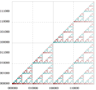
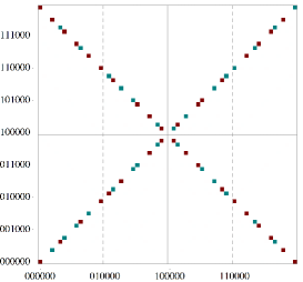
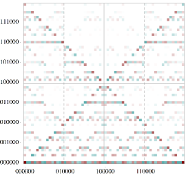
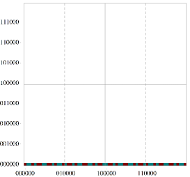
As an example, we provide in figure 26 images illustrating the ITF quantum phase transition: above, $\Gamma$ is small and only correlations in the $Z$-axis are relevant. Below, $\Gamma$ is large and correlations appear only in the $X$-axis. The middle panel shows the critical case.

Figure 26: Frame representation for $N=6$ qubits in the ground state of the AF ITF Hamiltonian 6 with PBC. The top panel shows the case where $\Gamma\to 0$, and correlations are established in the $Z$-axis. The central panel is critical, $\Gamma=1$ and the lower one shows the $\Gamma\to\infty$ case, where correlations are strong in the $X$-axis.

8 Conclusions and further work

In this work we have described a family of schemes which allow visualization of the information contained in quantum many-body wavefunctions, focusing on systems of many qubits. The schemes are self-similar by design: addition of new qubits results in a higher resolution of the plots. The thermodynamic limit, therefore, corresponds to the continuum limit.

The philosophy behind the schemes is to start out with a region $D$ and divide it into several congruent subdomains, all of them similar to $D$. This subdivision procedure can be iterated as many times as needed, producing an exponentially large amount of subdomains, each of them characterized by a geometrical index. This index can be now associated to an element of the tensor-basis of the Hilbert space, and its corresponding wavefunction amplitude goes, through a certain color code, into that subdomain. The most simple example is with $D$ a square which splits into four equal quadrants, but we can also start with a right triangle, or even with a line segment.

Physical features of the wavefunctions translate naturally into visual features of the plot. For example, within the scheme in section 2, the spin-liquid character of the ground state of the Heisenberg model shows itself in a characteristic pattern of diagonal lines. This pattern is able to distinguish between open and periodic boundary conditions. Other features which show up in the plots is magnetization, criticality, invariance under translations or permutation of the qubits, and Marshall’s sign rule. We have analysed the characteristic features of product states, the ground states of the Ising model in a transverse field, the Majumdar-Ghosh Hamiltonian or Dicke states. We have also studied spin-1 systems, such as the AKLT state.

A very relevant physical feature which becomes apparent in the plots is entanglement. Factorizability is straightforward to spot: a wavefunction is factorizable if all sub-images at a certain division level are equal, modulo normalization. The Schmidt rank of a given left-right partition of the system is related to the dimension of the subspace spanned by all sub-images within the corresponding subdivision of the plot and, so, a crude method to obtain an upper bound is to count the number of different sub-images. The full information about entanglement is contained in the matrix that we have termed as cross-correlation, which contains the overlap between all subimages at a certain division level.

In a very different spirit, we have illustrated the frame representations of quantum states of many qubits. This approach is related to Wooters’ group ideas. In it, the expectation values of a selected set of operators are shown in a 2D array, which is again displayed in a self-similar manner.

In this work we have taken the first steps in the exploration of an alternative strategy in the study of quantum many-body sytems, which can provide support to the corpus of methods in the field. Regarding further work, we would like to stress the further exploration of interesting quantum many-body states which we have not done here, for example the ground states of fermionic Hamiltonians, the Hubbard model, the Mott transition or the BEC-BCS crossover. Understanding the plotting structure of matrix product states of low dimension might also result profitable. Moreover, the mathematical properties of the mapping itself are worth studying by themselves.

As a final remark, we would like to announce that source code and further images can be found at http://qubism.wikidot.com, a webpage dedicated to qubism-related resources.

References

- [1] Chun-houh Chen, Wolfgang Karl Härdle, and Antony Unwin. Handbook of Data Visualization. Springer, 2008.
- [2] Edward R. Tufte. The Visual Display of Quantitive Information. Graphics Press, 2009.
- [3] H.J. Jeffrey. Chaos game representation of gene structure. Nucleic Acids Research, 18:2163, 1990.
- [4] Jonas S. Almeida, João A. Carriço, António Maretzek, Peter A. Noble, and Madilyn Fletcher. Analysis of genomic sequences by chaos game representation. Bioinformatics, 17:429, 2001.
- [5] Na Liu and Tianming Wang. Graphical representation for protein secondary structure sequences and their application. Chem. Phys. Lett., 435:127, 2007.
- [6] Bai-lin Hao, H.C. Lee, and Shu-yu Zhang. Fractals related to long dna sequences and complete genomes. Chaos, Solitons & Fractals, 11:825, 2000.
- [7] Jose I. Latorre. Image compression and entanglement. 2005.
- [8] Phuc Le, Fangyan Dong, and Kaoru Hirota. A flexible representation of quantum images for polynomial preparation, image compression, and processing operations. Quantum Information Processing, 10:63–84, 2011.
- [9] E. Majorana. Atomi orientati in campo magnetico variabile. Il Nuovo Cimento, 9:43–50, 1932.
- [10] Martin Aulbach, Damian Markham, and Mio Murao. The maximally entangled symmetric state in terms of the geometric measure. New Journal of Physics, 12(7):073025, 2010.
- [11] Wojciech Ganczarek, Marek Kuś, and Karol Życzkowski. Barycentric measure of quantum entanglement. Phys. Rev. A, 85:032314, Mar 2012.
- [12] Kathleen S. Gibbons, Matthew J. Hoffman, and William K. Wootters. Discrete phase space based on finite fields. Phys. Rev. A, 70:062101, Dec 2004.
- [13] Subir Sachdev. Quantum phase transitions. Cambridge University Press, 2001.
- [14] Maciej Lewenstein, Anna Sanpera, and Verònica Ahufinger. Ultracold atoms in optical lattices. Oxford University Press, 2012.
- [15] W. Marshall. Antiferromagnetism. Proc. Roy. Soc. A, 232:48–68, 1955.
- [16] John K. Stockton, J. M. Geremia, Andrew C. Doherty, and Hideo Mabuchi. Characterizing the entanglement of symmetric many-particle spin- systems. Phys. Rev. A, 67:022112, Feb 2003.
- [17] Ian Affleck, Tom Kennedy, Elliott H. Lieb, and Hal Tasaki. Valence bond ground states in isotropic quantum antiferromagnets. Communications in Mathematical Physics, 115:477–528, 1988. 10.1007/BF01218021.
- [18] F. D. M. Haldane. Nonlinear field theory of large-spin heisenberg antiferromagnets: Semiclassically quantized solitons of the one-dimensional easy-axis néel state. Phys. Rev. Lett., 50:1153–1156, Apr 1983.
- [19] Marcel den Nijs and Koos Rommelse. Preroughening transitions in crystal surfaces and valence-bond phases in quantum spin chains. Phys. Rev. B, 40:4709–4734, Sep 1989.
- [20] David Perez-Garcia, Frank Verstraete, J. Ignacio Cirac, and Michael M. Wolf. Peps as unique ground states of local hamiltonians. Quant.Inf.Comp., 8:0650, 2008.
- [21] Manfred Schroeder. Fractals, chaos, power laws. W. H. Freeman, 1992.
- [22] Albert Einstein. The Einstein-Born letters; Correspondence between Albert Einstein and Max and Hedwig Born from 1916 to 1955. Walker, 1971.
- [23] Michael A. Nielsen and Isaac L. Chuang. Quantum computation and quantum information. Cambridge University Press, 2004.
- [24] G. Vidal, J. I. Latorre, E. Rico, and A. Kitaev. Entanglement in quantum critical phenomena. Phys. Rev. Lett., 90:227902, Jun 2003.
- [25] Heng Fan, Vladimir Korepin, and Vwani Roychowdhury. Entanglement in a valence-bond solid state. Phys. Rev. Lett., 93:227203, Nov 2004.
- [26] Christopher Ferrie and Joseph Emerson. Frame representations of quantum mechanics and the necessity of negativity in quasi-probability representations. Journal of Physics A: Mathematical and Theoretical, 41(35):352001, 2008.
- [27] Christopher Ferrie. Quasi-probability representations of quantum theory with applications to quantum information science. Reports on Progress in Physics, 74(11):116001, 2011.
- [28] Robert W. Spekkens. Negativity and contextuality are equivalent notions of nonclassicality. Phys. Rev. Lett., 101:020401, Jul 2008.