The onset of high-mass star formation in the direct vicinity of the galactic mini-starburst W43

Abstract

Context. The earliest stages of high-mass star formation are still poorly characterized. Densities, temperatures and kinematics are crucial parameters for simulations of high-mass star formation. It is also unknown whether the initial conditions vary with environment.

Aims. We want to investigate the youngest massive gas clumps in the environment of extremely active star formation.

Methods. We selected the IRDC 18454 complex, directly associated with the W43 Galactic mini-starburst, and observed it in the continuum emission between 70 $\mu$m and 1.2 mm with Herschel, APEX and the 30 m telescope, and in spectral line emission of N₂H⁺ and ¹³CO with the Nobeyama 45 m, the IRAM 30 m and the Plateau de Bute Interferometer.

Results. The multi-wavelength continuum study allows us to identify clumps that are infrared dark even at 70 $\mu$m and hence the best candidates to be genuine high-mass starless gas clumps. The spectral energy distributions reveal elevated temperatures and luminosities compared to more quiescent environments. Furthermore, we identify a temperature gradient from the W43 mini-starburst toward the starless clumps. We discuss whether the radiation impact of the nearby mini-starburst changes the fragmentation properties of the gas clumps and by that maybe favors more high-mass star formation in such an environment. The spectral line data reveal two different velocity components of the gas at 100 and 50 km s^-1. While chance projection is a possibility to explain these components, the projected associations of the emission sources as well as the prominent location at the Galactic bar – spiral arm interface also allow the possibility that these two components may be spatially associated and even interacting.

Conclusions. High-mass starless gas clumps can exist in the close environment of very active star formation without being destroyed. The impact of the active star formation sites may even allow for more high-mass stars to form in these 2nd generation gas clumps. This particular region near the Galactic bar – spiral arm interface has a broad distribution of gas velocities, and cloud interactions may be possible.

1 Introduction

The initial conditions required to form massive stars is one of the major topics in high-mass star formation research today. The advent of new observational capabilities often opened the window to earlier and earlier evolutionary stages in that field. While the IRAS satellite combined with cm continuum surveys of the galactic plane revealed the populations of ultracompact Hii regions and high-mass protostellar objects (HMPOs, e.g., Wood & Churchwell 1989a, b; Kurtz et al. 1994; Molinari et al. 1996; Sridharan et al. 2002), the advent of the mid-infrared satellites ISO, MSX and Spitzer allowed to access even earlier evolutionary stages, namely the infrared dark clouds (IRDCs, e.g., Perault et al. 1996; Egan et al. 1998; Carey et al. 2000; Sridharan et al. 2005; Simon et al. 2006; Peretto & Fuller 2009). However, it turned out that most of the so far studied IRDCs host weak 24 $\mu$m emission sources and drive molecular outflows, both strong indicators for star formation activity (e.g., Beuther et al. 2005b; Beuther & Steinacker 2007; Beuther & Sridharan 2007; Rathborne et al. 2006; Motte et al. 2007; Cyganowski et al. 2008). Therefore, we are still lacking a thorough understanding of the initial conditions for high-mass star formation prior to any star formation activity. The advent of the Herschel far-infrared satellite (Pilbratt et al., 2010) now offers the unique opportunity to identify targets for these initial conditions and to study their physical and chemical properties in detail. Major characteristics of these earliest evolutionary stages are, that the massive gas cores with masses in excess of several 100 M_⊙ observed at (sub)mm wavelengths are still dark at 70 $\mu$m, hence they have not formed any protostellar objects to Herschel sensitivity limits yet.

The Herschel guaranteed time key project EPOS (Early Stages of Star Formation, P.I. O. Krause) is a dedicated observation campaign targeting 45 IRDCs that are promising candidates to search for and to study these initial conditions. Early results from the first data revealed already exciting results, e.g., we identified candidate high-mass starless cores (HMSCs) as well as very weak 70 $\mu$m sources within IRDCs that may be the very first manifestation of high-mass star formation (Beuther et al., 2010; Henning et al., 2010; Linz et al., 2010).

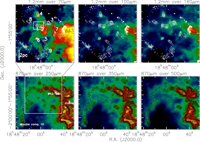
Figure 1: Compilation of the continuum data from 70 $\mu$m to 1.2 mm wavelength as labeled in each panel. The top-row presents the data on a smaller spatial scale as marked in the bottom-left panel. The color-scale is chosen in each image individually to highlight the most important features. Contour levels of the 870 $\mu$m data start at the 3$\sigma$ levels of 0.27 mJy beam^-1 and continue in in 3$\sigma$ steps to 2.7 Jy beam^-1, from where they continue in 2.7 Jy beam^-1 steps. The 1.2 mm data are contoured in 3$\sigma$ levels of 30 mJy beam^-1. The numbers in the top-left panel label the sub-cores, the white small box there marks the region shown in Fig. 5, and a scale-bar for a distance of 5.5 kpc is shown as well. The crosses in the bottom-left panel mark the positions of a double-component radio recombination line Hii region from Anderson et al. (2011), the W43-MM1 position from Motte et al. (2003) as well as the approximate center of the Wolf-Rayet/OB cluster (Blum et al., 1999; Motte et al., 2003).

The IRDC 18454 close to W43:

One particularly interesting region within the sample are the IRDCs associated with the IRAS source IRAS 18454-0158. Henceforth, we will call the region IRDC 18454. While the IRAS source was first studied in the framework of the HMPO survey by Sridharan et al. (2002) and Beuther et al. (2002), it was soon recognized that several of the sub-sources are indeed infrared dark (Sridharan et al., 2005). Another curiosity of that region is that it harbors two distinctly different velocity components, one around 50 and one around 100 km s^-1 (Sridharan et al., 2005; Beuther & Sridharan, 2007). It is also interesting to note that only the 100 km s^-1 component shows SiO emission, indicative of a molecular outflow, whereas we do not detect any SiO from the 50 km s^-1 component (Beuther & Sridharan, 2007). Furthermore, the measured H¹³CO⁺(1–0) line-width from the 100 km s^-1 component is also broader than that at 50 km s^-1 (2.7 versus 1.7 km s^-1, Beuther & Sridharan 2007), also indicating that the 50 km s^-1 component is in a less turbulent state. The kinematic distances derived by Beuther & Sridharan (2007) for the 50 and 100 km s^-1 components, using the Brand & Blitz (1993) rotation curve were 3.5 and 6.4 kpc, respectively. Applying the new rotation curve by Reid et al. (2009), we now get kinematic distances of 3.3 and 5.5 kpc for both components, respectively. The 5.5 kpc distance corresponds well to the distance derived for the large Hii region W43 by Wilson et al. (1970). A similar distance of $\sim 6$ kpc was also recently derived for the nearby red supergiant cluster RSGC3 (Negueruela et al., 2011)). We will discuss later whether these are really two different components just chance-projected together on the plane of the sky, or whether it may be interacting cloud components at similar distances.

In the direct vicinity of that region we find the large Galactic mini-starburst region W43 (Fig. 1), which was already studied in detail in the past with a broad wavelength coverage (e.g., Smith et al. 1978; Lester et al. 1985; Blum et al. 1999; Motte et al. 2003; Nguyen Luong et al. 2011) including also early Herschel results (Bally et al., 2010; Elia et al., 2010). The IRDC 18454 is located at the northeastern edge of the Z-shaped filament first discussed in Motte et al. (2003) (see also Fig. 1). This region is very luminous with $L\sim 3\times 10^{6}$ L_⊙, and it contains sources at different evolutionary stages from a Wolf-Rayet cluster to active young star-forming cores (e.g., Blum et al. 1999; Motte et al. 2003). Nguyen Luong et al. (2011) recently discussed several broad velocity components in that regions and suggested that this whole complex might have formed via converging gas flows due to its special location at the interface of the Galactic bar with the inner Scutum spiral arm (Benjamin et al., 2005; López-Corredoira et al., 2007; Rodriguez-Fernandez & Combes, 2008). Different velocity components were also identified in atomic HI emission and absorption (Liszt et al., 1993). However, our target region IRDC 18454 which hosts supposedly the earliest evolutionary stages, has not been subject to a detailed investigation yet.

Among others, we like to address the following questions: Do we identify bona-fide high-mass starless cores at all? If yes, what are their physical properties, e.g., their temperatures and turbulent line-widths? Are the two velocity components spatially associated or are they rather chance alignments along the line of sight? Does the mini-starburst W43 impose any impact on the earliest evolutionary stages or are the young cores evolving independently of that? Do we find any signature of triggering?

2 Observations and archival data

2.1 Herschel

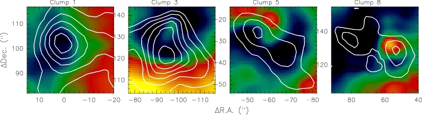
Figure 2: Zoom into the 70 $\mu$m dark cores with 1.2 mm continuum contours on the 70 $\mu$m color-scale emission. The color-scale is again chosen to highlight the most important features. The 1.2 mm data are contoured in 3$\sigma$ levels of 30 mJy beam^-1. The 0 position is at R.A. (J2000.0)18:48:02.160 and Dec. (J2000.0) -01:55:38.0.

The cloud complex with a size of $\sim 6^{\prime}\times 6^{\prime}$ was observed with PACS (Poglitsch et al., 2010) on Herschel (Pilbratt et al., 2010) on 2010 March 9. Scan maps in two orthogonal directions with scan leg lengths of $18^{\prime}$ and $6^{\prime}$, respectively, were obtained with the medium scan speed of $20^{\prime\prime}$/s. The raw data have been reduced up to level-1 with the HIPE software (Poglitsch et al., 2010; Ott, 2010), version 6.0, build 1932. Besides the standard steps, we applied a 2^ndlevel deglitching, in order to remove bad data values from a given pixel map by $\sigma$-clipping the flux values which contribute to each pixel. We used the time-ordered option and applied a 25$\sigma$ threshold. The final level-2 maps were processed using Scanamorphos version 8 (Roussel 2011, subm.). Since the field of view contains bright emission on scales larger than the map, we applied the “galactic” option and included the non-zero-acceleration telescope turn-around data. The flux correction factors provided by the PACS ICC team were applied.

Maps at 250, 350, and 500 $\mu$m were obtained with SPIRE (Griffin et al., 2010) on 2010 March 11. Two $14^{\prime}$ scan legs were used to cover the source. The data were processed up to level-1 within HIPE, developer build 5.0, branch 1892, calibration tree 5.1 using the standard photometer script (POF5_pipeline.py, dated 2.3.2010) provided by the SPIRE ICC team. The resulting level-1 maps have been further reduced using Scanamorphos, version 9 (patched, dated 08.03.2011). This version included again the essential de-striping for maps with less than 3 scan legs per scan. In addition, we used the “galactic” option and included the non-zero-acceleration telescope turn-around data. Color corrections were applied according to the SPIRE Manual.

2.2 Plateau de Bure Interferometer

We observed IRDC 18454-1 with the Plateau de Bure Interferometer during five nights in October and November 2009 at 93 GHz in the C and D configurations covering projected baselines between approximately 13 and 175 m. The 3 mm receivers were tuned to 92.835 GHz in the lower sideband covering the N₂H⁺(1–0) as well as the 3.23 mm continuum emission. For continuum measurements we placed six 320 MHz correlator units in the band, the spectral lines were excluded in averaging the units to produce the final continuum image. Temporal fluctuations of amplitude and phase were calibrated with frequent observations of the quasars 1827+062 and 1829-106. The amplitude scale was derived from measurements of MWC349 and 3c454.3. We estimate the final flux accuracy to be correct to within $\sim 15\%$. The phase reference center is R.A. (J2000.0) 18:48:02.21 and Dec. (J2000.0) -01:53:55.79, and the velocity of rest $v_{\rm{lsr}}$ is $\sim$51.9 and 99.6 km $s^{-1}$ for the two velocity components, respectively. The synthesized beam of the line and continuum data is $3.9^{\prime\prime}\times 3.2^{\prime\prime}$ with a P.A. of 34 degrees. The $3\sigma$ continuum rms is 0.27 mJy beam^-1. The $3\sigma$ rms of the N₂H⁺(1–0) data measured from an emission-free channel with a spectral resolution of 0.2 km s^-1 is 21 mJy beam^-1.

2.3 Nobeyama 45 m telescope

The N₂H⁺ data has been observed using the BEARS receiver at the NRO 45 m telescope in Nobeyama, Japan. The receiver has been tuned to $93.17346$ MHz, covering the full hyperfine structure of the N₂H${}^{+}(1-0)$ transition. At this frequency the telescope beam is $18.2^{\prime\prime}$ and the observing mode provides a spectral resolution of $0.2$ km s^-1 at a bandwidth of 32 MHz. The different velocity components have been observed one in April 2010 with an average system temperature of $T_{\rm{sys}}=206$ K, the second in June, at slightly lower $T_{\rm{sys}}$ . The software package nostar (Sawada et al., 2008) was used for the data reduction, sampling the data to a pixel size of $7^{\prime\prime}$ with a spheroidal convolution and smoothing the spectral resolution to $0.5$ km s^-1. The rms of the final map is $\sim 0.125$ K and $\sim 0.09$ K for the 100 km s^-1 and 50 km s^-1 map, respectively. Strong winds hampered the pointing for part of the observations, contributing to spatial uncertainties.

2.4 Archival data from Spitzer, APEX and the IRAM 30 m

The MIPS 24 $\mu$m data (from MIPSGAL, Carey et al. 2009) as well as the IRAC 8 $\mu$m observations (from GLIMPSE, Churchwell et al. 2009) are taken from the Spitzer archive. The 1.2 mm continuum data were first presented in Beuther et al. (2002) and the APEX 870 $\mu$m data are part of the ATLASGAL survey of the Galactic plane (Schuller et al., 2009). Beam sizes of the two datasets are $10.5^{\prime\prime}$ and $19.2^{\prime\prime}$, respectively. The $1\sigma$ rms values are 10 and 90 mJy beam^-1, respectively.

3 Results

3.1 Continuum emission

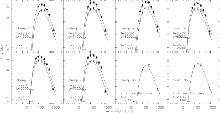
Figure 3: Spectral energy distributions (SEDs) of the discussed clumps. The fluxes are extracted for apertures of $36.6^{\prime\prime}$ and $19.2^{\prime\prime}$. For clumps 8a and 8b only the smaller apertures of $19.3^{\prime\prime}$ were used. Error bars represent 20% uncertainties. Each panel lists the corresponding temperatures $T$ and bolometric luminosities $L$ for both fits top and bottom, respectively. Clumps 1, 3 and 8a are starless clump candidates.

Figure 1 gives an overview of the target regions in all accessible continuum bands from the far-infrared at 70 $\mu$m to the 1.2 mm band. The bottom panel of Fig. 1 shows the large-scale emission covering prominently the Z-shaped strong submm emission from the mini-starburst region W43 in the west of the images. The morphology of all images longward of 250 $\mu$m wavelengths agrees well in all bands. While these data would also allow us an analysis of the W43 region itself (see also Bally et al. 2010), for this project we concentrate on the earliest evolutionary stages in the north-eastern part of the region highlighted in the top panels of Fig. 1. The high spatial resolution of the Herschel PACS images between 70 and 160 $\mu$m (between $\sim$5.6^′′, $\sim$6.8^′′ and $\sim$11.4^′′) and the 1.2 mm map from the IRAM 30 m ($\sim$10.5^′′) allow us to spatially differentiate different components. While the long-wavelength data from 250 $\mu$m onwards are structurally similar, a spatial comparison of the 70 $\mu$m with the 1.2 mm data shows significant differences. In simple terms, the emission longward of 250 $\mu$m is largely dominated by the cold dust from the natal gas and dust clump, whereas the emission shortward of 100 $\mu$m becomes dominated by warmer dust components, which may be heated by internal early star formation processes. Some of the mm clumps exhibit strong mid-infrared emission whereas others are either weak or show no emission at all at 70 $\mu$m. This is in contrast to the neighboring W43 region, which is strong in all wavelengths covered here. This already outlines the different evolutionary stages of the main W43 region and the infrared dark gas clumps we are investigating here.

Table 1: Clump parameters from the 1.2 mm data

#	R.A.	Dec.	$S_{\rm{peak}}$	$S$	N${}_{\rm{H}_{2}}$	$M$
	(J2000.0)	(J2000.0)	$\left(\frac{\rm{mJy}}{\rm{beam}}\right)$	(mJy)	$\left(\frac{10^{23}}{\rm{cm}^{2}}\right)$	(M⊙)
1	18:48:02.23	-01:53:56.4	178	479	1.6	609
2	18:47:59.99	-01:54:07.5	157	468	1.4	595
3	18:47:55.86	-01:53:36.8	203	816	1.8	1037
4	18:48:01.56	-01:52:30.9	175	491	1.6	624
5a	18:47:58.50	-01:56:03.9	102	125	0.9	159
5b	18:47:57.68	-01:56:13.9	88	169	0.8	215
6	18:48:02.28	-01:55:43.2	87	108	0.8	137
7	18:47:52.21	-01:54:54.5	100	123	0.9	156
8a	18:48:07.60	-01:53:21.6	81	108	0.7	137
8b	18:48:05.74	-01:53:28.5	103	178	0.9	226

Considering an evolutionary sequence, the youngest sources without internal heating sources should be dark even at 70 $\mu$m wavelength. As soon as a central core/protostar starts producing its own luminosity either by accretion shocks or nuclear synthesis, emission at 70 $\mu$m, 24 $\mu$m and at shorter wavelengths will become detectable (e.g., Beuther et al. 2010; Henning et al. 2010; Motte et al. 2010). To examine the youngest starless candidate clumps in more detail, Figure 2 presents zoomed in images of the selected mm clumps that show no or only weak 70 $\mu$m emission. The 1.2 mm emission peaks of clumps 1, 3, 5a, 8a and 9 are all non-detections at 70 $\mu$m wavelengths. However, there are subtle differences between the clumps. For example, clump 1 is a clear 70 $\mu$m absorption feature whereas clump 3 shows 70 $\mu$m emission associated with the north-eastern extension of the 1.2 mm cold dust emission. While this indicates that clump 1 is likely still in a starless evolutionary phase, star formation may have already started in clump 3, although the column density peak still appears devoid of active star formation signatures.

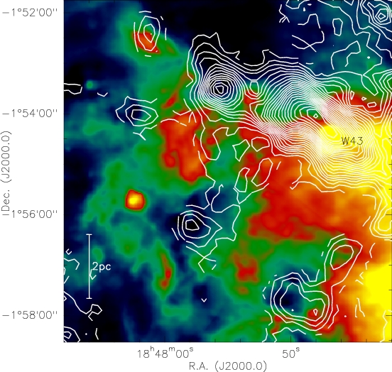
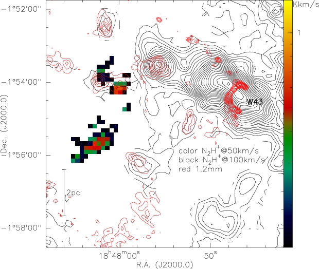
Figure 4: Left: N₂H⁺(1–0) contours over 70 $\mu$m emission. The color-scale is again chosen to highlight the most important features. The N₂H⁺ emission is integrated from 91 to 106 km s^-1, and contours start at 0.6 and continue in 1 K km s^-1 levels. Right: N₂H⁺(1–0) and 1.2 mm emission. The color-scale shows the N₂H⁺ emission integrated from 49 to 53 km s^-1 and the black contours present the N₂H⁺ emission integrated from 91 to 106 km s^-1. The contours start at 0.6 and continue in 1 K km s^-1 levels. The red 1.2 mm emission is contoured in 3$\sigma$ levels of 30 mJy beam^-1. Scale-bars are shown at the bottom-right of each panel.

Assuming optically this dust continuum emission at (sub)mm wavelengths at a typical temperature of 20 K (see section 3.2) with a dust opacity index $\beta=2$ (corresponding to $\kappa_{\rm{1.2mm}}\sim 0.4$ cm²g^-1 representing the general ISM, e.g., Mathis et al. 1977; Ossenkopf & Henning 1994), we can calculate the clump masses and peak column densities following the classical approach by Hildebrand (1983). An adaptation of the equations can be found in Beuther et al. (2002, 2005a). The resulting values derived from the 1.2 mm data are presented in Table 1. Although the derived masses are uncertain by about a factor 5 based on mainly temperature, $\beta$ and gas-to-dust mass ratio uncertainties (e.g., Ossenkopf & Henning 1994; Beuther et al. 2002; Draine et al. 2007), nevertheless, the average clump masses are relatively high. If one assumes an initial mass function (IMF) following Kroupa (2001) with an approximate star formation efficiency of 30%, the initial gas clumps should have masses in excess of 1000 M_⊙ in order to be capable to form at least one 20 M_⊙ star. In this picture, at least clump 1 can be considered as one of the best candidates of being a high-mass starless clump. Clump 3 also full-fills the mass criteria, but it exhibits two point sources at the edge of the clump, hence some star formation activity may have just started. Nevertheless, clump 3 should also be in a very young evolutionary stage and resemble the initial conditions of high-mass star formation well.

The estimated column densities based on the 30 m single dish data are in the regime $0.7-1.8\times 10^{23}$ cm^-2 (Table 1). While this is slightly below the typically discussed threshold of $\sim$1 g cm^-2 (e.g., Krumholz & McKee 2008, corresponding to $\sim$3$\times 10^{23}$ cm^-2) this is certainly no counterargument since these are average values of the beam size of $10.5^{\prime\prime}$ that corresponds to linear spatial scales of approximately 58000 AU or a quarter of a pc. Higher resolution observations will reveal significantly larger column densities (section 3.4). Therefore, also from that point of view, the regions qualify as likely extremely young high-mass star-forming regions.

3.2 Spectral energy distributions (SEDs)

The Herschel data allow us to extract SEDs for the gas and dust clumps, and by that to determine the bolometric luminosities and temperatures. Since we are targeting very young regions that are not detected as point sources in the Herschel bands, classical PSF-photometry or point source flux extraction where the background is subtracted is difficult. Furthermore, we like to include all Herschel bands for our SED fits. Therefore, we extract the peak fluxes at all wavelengths from maps smoothed to the $36.6^{\prime\prime}$ beam of the 500 $\mu$m data. Furthermore, we also extract the peak fluxes from maps smoothed to the $19.2^{\prime\prime}$ resolution of the 870 $\mu$m ATLASGAL data, ignoring the 350 and 500 $\mu$m maps then. Since clumps 8a and 8b are too close to be separated by the $36.6^{\prime\prime}$ beam, for these clumps we only use the $19.2^{\prime\prime}$ maps. For clumps 5a and 5b, where even at 250 $\mu$m the two peaks merge into one, no proper flux determination was possible. At the assumed distance of 5.5 kpc, the apertures of $36.6^{\prime\prime}$ and $19.2^{\prime\prime}$ correspond to linear apertures of $\sim 1$ pc and $\sim 0.5$ pc, respectively.

One inherent problem in flux measurements from Herschel data is that the diffuse Galactic background level is unknown and therefore hard to correct for. In particular in a region like the one presented here where at all wavelengths significant emission is seen throughout the whole maps. One should note that the problem is more severe when targeting very young or starless regions that do not exhibit clear point sources, because for more evolved point-source like structure, proper PSF-photometry better allows to subtract a background level. To approximate a background level, we define polygons at the map edges with low emission regions. The mean of these regions is then subtracted from our measured fluxes.

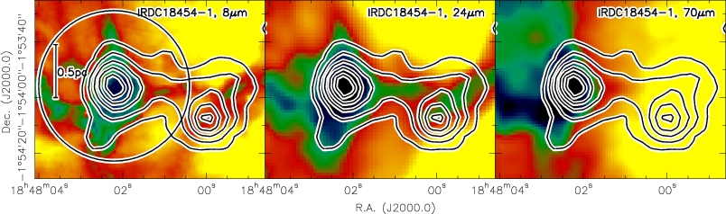
Figure 5: Zoom into the two central clumps 1 and 2 (see Fig. 1). The left and middle panels present in color-scale the Spitzer 8 and 24 $\mu$m emission, whereas the right panel shows the Herschel 70 $\mu$m image. Color-scale is again to highlight the main features with dark low and yellow high intensities. The contours show the 1.2 mm continuum emission contoured in 3$\sigma$ levels of 30 mJy beam^-1. The circle outlines the FWHM of the primary beam of the PdBI observations, and a scale-bar is shown in the left panel as well.

The SEDs were fitted using modified blackbody functions accounting for the wavelength-dependent emissivity of the dust. The assumed dust composition follows Ossenkopf & Henning (1994) with thin ice mantles, and the assumed gas-to-dust mass ratio is 100. Figure 3 presents the SEDs of all clumps (except 5a and 5b) as derived for the apertures of $36.6^{\prime\prime}$ and $19.2^{\prime\prime}$. While the overall spread of fitted dust temperatures is relatively low (between $\sim$18 and $\sim$26 K), we identify on average lower temperatures toward the mid-infrared dark clumps 1, 3 and 8 (19 to 20 K) compared to the clumps with embedded objects (21 to 28 K).

We compared the temperatures derived from our SED fitting (here and section 4.1) with the temperature map recently produced by Battersby et al. (2011). The main differences between the two datasets is that Battersby and collaborators used the HIGAL data (Molinari et al., 2010), and they were able to subtract a background in a systematic fashion because of the much larger spatial coverage. The temperature comparison shows that in the low-$T$ regime ($\leq 25$ K) the temperatures agree very well, whereas in the high-$T$ regime ($\geq 30$ K) our analysis underestimates their temperatures. Since here we are mainly interested in the cold gas clumps, our approach is perfectly justifiable.

The other important parameter one can derive from the SEDs is the bolometric luminosities of the regions. As expected, for smaller apertures one finds lower bolometric luminosities. Nevertheless, it is interesting to note that toward almost all clumps we find bolometric luminosities in excess of 1000 L_⊙ (except clump 8a). This is particularly surprising for the two starless clump candidates 1 and 3 that exhibit luminosities of 1200 and 1800 L_⊙, respectively, even measured within the smaller apertures of $\sim$0.5 pc size. We will come back to this in section 4.1.

3.3 Kinematic properties from N₂H⁺

With the initial single-pointing spectra from Sridharan et al. (2005) one could not associate the different velocity components spatially well with the sub-clumps of the region. With the new N₂H⁺(1–0) maps at large scales (Fig. 4) as well as small scales (see section 3.4) we now can study the kinematics of the gas in much more detail. Figure 4 presents an overview of the integrated N₂H⁺(1–0) components around 100 and 50 km s^-1, respectively. The left panel of Figure 4 presents the N₂H⁺ relation with the 70 $\mu$m warm dust emission whereas the right panel presents the relation to the 1.2 mm cold dust emission. We find strong N₂H⁺ emission of the 100 km s^-1 component toward the already very active W43 region and the younger regions still dark at 70 $\mu$m without any obvious preference between them. In contrast to that, the 50 km s^-1 component is absent toward the W43 complex but just exhibits emission associated with three clumps of the IRDC 18454. Of particular interest are the two central clumps 1 and 2 which at the spatial resolution of the Nobeyama data appear to exhibit emission from both components simultaneously. As shown in the following section, this is not exactly true but we can associate the two clumps with individual velocity components.

Independent of this, the question arises whether these two velocity components are just chance alignments along the line of site or whether they are spatially related and may even indicate some cloud-cloud interaction. Could such a cloud-cloud interaction arise in the interface region of the Galactic bar and the beginning of the spiral arm where this region is located? We will come back to this question in section 4.2.

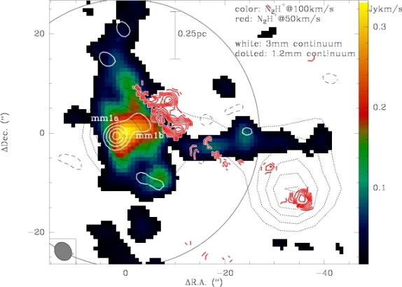
Figure 6: PdBI 3 mm of the clumps 1 and 2. The color-scale shows the integrated N₂H⁺(1–0) emission within the velocity interval from 90.5 to 94.5 km s^-1 whereas the red contours present the N₂H⁺(1–0) emission within the velocity interval from 43.8 to 45.6 km s^-1. The white contours show the corresponding 3.2 mm continuum emission contoured from the 3$\sigma$ level in 2$\sigma$ steps (1$\sigma=$0.27 mJy beam^-1). The full circle outlines that FWHM of the PdBI primary beam at the given frequency, and a scale-bar is shown as well. The PdBI synthesized beam is presented at the bottom-left. The dotted contours show the 1.2 mm continuum emission contoured in 3$\sigma$ levels of 30 mJy beam^-1.

3.4 Zooming into the 2 central clumps

3.4.1 Millimeter continuum emission

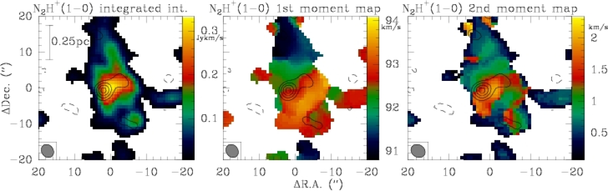
Figure 7: The color-scale shows the 0th, 1st and 2nd moment map of the N₂H⁺(1–0) emission in the velocity regime between 90.5 and 94.5 km s^-1 (corresponding to the integrated intensity, the intensity-weighted peak velocity and the intensity-weighted line-width, respectively). The contours present the 3.2 mm continuum emission contoured from the 3$\sigma$ level in 2$\sigma$ steps (1$\sigma=$0.27 mJy beam^-1). The left panel shows a scale-bar, and the PdBI synthesized beam is presented at the bottom-left of each panel. The 0/0 position is the phase center of the PdBI observations at R.A. (J2000.0) 18:48:02.21 and Dec, (J2000.0) -01:53:55.8.

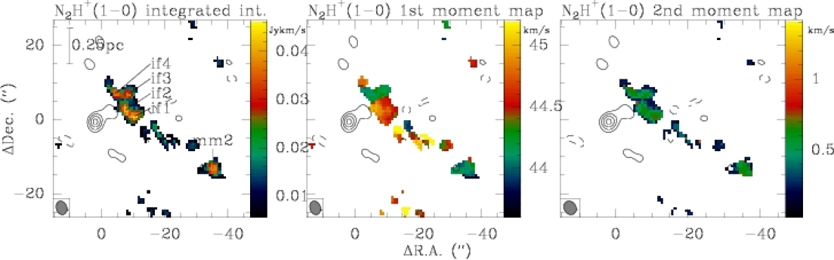
Figure 8: The color-scale shows the 0th, 1st and 2nd moment map of the N₂H⁺(1–0) emission in the velocity regime between 43.8 and 45.6 km s^-1 (corresponding to the integrated intensity, the intensity-weighted peak velocity and the intensity-weighted line-width, respectively). The contours present the 3.2 mm continuum emission contoured from the 3$\sigma$ level in 2$\sigma$ steps (1$\sigma=$0.27 mJy beam^-1). The four interface positions if1 to if4 and the peak associated with clump 2 are marked in the left panel. The left panel shows a scale-bar, and the PdBI synthesized beam is presented at the bottom-left of each panel. The 0/0 position is the phase center of the PdBI observations at R.A. (J2000.0) 18:48:02.21 and Dec, (J2000.0) -01:53:55.8.

Figure 5 presents a zoom into the central region covering the two clumps 1 and 2. While both mm emission clumps are very similar at mm wavelength as well as at 8 and 24 $\mu$m, clump 2 starts as an emission source from 70 $\mu$m onwards whereas clump 1 is still dark at these far-infrared wavelengths. This difference is also manifested in SEDs (Fig. 3) where temperature and luminosity of clump 1 are lower than the corresponding values for clump 2. This indicates an earlier evolutionary stage for clump 1. Figure 5 also shows the FWHM of the primary beam of our PdBI observations which was centered on clump 1. However, one should keep in mind that this circle represents only the FWHM, and that the PdBI can also trace structures outside of that (see below).

The PdBI 3.23 mm continuum and N₂H⁺ data now allow us a more detailed characterization of in particular clump 1, but to a lower level also of clump 2. Figure 7 presents the integrated 100 and 50 km s^-1 N₂H⁺ emission as well as the 3.23 mm continuum data. At the higher spatial resolution of $\sim 3.6^{\prime\prime}$, that corresponds to linear scales of $\sim 20000$ AU ($\approx 0.1$ pc), clump 1 resolves into two cores, one being the dominant and primary component. The projected separation between the 2 cores is $\sim 5.5^{\prime\prime}$, corresponding to a projected linear separation of $\sim 30000$ AU (or $\sim 0.15$ pc). This is consistent with the typical Jeans-length of $\sim$0.1 pc for a gas clump at 20 K with an average density of $10^{5}$ cm^-3. The assumed 3.23 mm continuum emission from clump 2 is too low to be detected at the edge of the primary beam of these PdBI observations (Fig. 6).

Peak and integrated fluxes as well as the corresponding gas column densities and masses (assuming again optically thin dust continuum emission at a temperature of 20 K, see section 3.1) are presented in Table 2. The two 3 mm cores add up to a total mass of $\sim$91 M_⊙, approximately 15% of the mass detected in the 1.2 mm single-dish data (Table 1). This difference can be attributed to the missing flux typically filtered out by interferometer observations. As already indicated in section 3.1, the interferometrically observed column densities are larger by about a factor 2 than the single-dish column densities.

Table 2: Core parameters from the PdBI 3.23 mm data

#	R.A.	Dec.	$S_{\rm{peak}}$	$S$	N${}_{\rm{H}_{2}}$	$M$
	(J2000.0)	(J2000.0)	$\left(\frac{\rm{mJy}}{\rm{beam}}\right)$	(mJy)	$\left(\frac{10^{23}}{\rm{cm}^{2}}\right)$	(M⊙)
1a	18:48:02.33	-01:53:56.3	0.9	1.1	3.0	59
1b	18:48:02.01	-01:53:53.8	0.4	0.6	1.4	32

3.4.2 N₂H${}^{+}(1-0)$ spectral line emission

The integrated N₂H${}^{+}(1-0)$ emission of the 100 and 50 km s^-1 components observed with the spatial resolution of the PdBI now for the first time allows us to spatially distinguish the origin of the different components. Figure 6 shows that the 100 km s^-1 component is closely related to the starless clump 1. Hence, this starless clump is spatially related to the western luminous mini-starburst complex W43 (e.g., Nguyen Luong et al. 2011). This is also observable by the filamentary extension of the 100 km s^-1 component toward the west, touching only the northern edge of clump 2.

In comparison to this, the 50 km s^-1 component is spatially located at the western edge of clump 1. The projected 50 km s^-1 component appears to directly touch the western edge of the 100 km s^-1 component. Technically a bit more surprising, we find a clear detection of the N₂H${}^{+}(1-0)$ 50 km s^-1 component toward the peak position of clump 2. And at a low level this 50 km s^-1 clump 2 emission is connected to the 50 km s^-1 component at the western edge of clump 1.

The visual impression one gets from the close spatial association of the 50 and 100 km s^-1 N₂H⁺ data is that these two velocity components, that are so strongly separated in velocity space, may still be spatially correlated on the sky and not just chance projections. It is also intriguing that the 1.2 mm peak fluxes and integrated fluxes as well as the projected spatial size of clumps 1 and 2 are so similar (Table 1). While chance projection of two gas clumps at different distances is obviously a possibility to explain all features, the whole W43 complex at the interface of the central bar of our Galaxy and the onset of the spiral arm is known to exhibit a large breadth of velocity components (Nguyen Luong et al., 2011). Therefore, a spatial association and even interaction between two complexes could be possible as well (see also section 3.3). We come back to this scenario in section 4.2.

Figures 7 and 8 present the three moment maps (integrated intensities, intensity-weighted peak velocities and intensity-weighted line widths) of the 100 and 50 km s^-1 components, respectively. For the 100 km s^-1 component we find a velocity gradient approximately perpendicular to the connecting axis of the two 3.23 mm peaks mm1a and mm1b. The broadest line width is also associated with the strongest mm peak mm1a. The 50 km s^-1 component does not exhibit a clear velocity gradient between mm2 and the interface region of mm1. Furthermore, the 2nd moment map does not show obvious line width increases toward one or the other position.

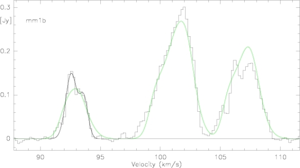
Figure 9: N₂H${}^{+}(1-0)$ spectra around 100 km s^-1 toward mm1a and mm1b. The green lines show N₂H⁺ fits taking into account the whole hyperfine structure whereas the black lines show two-component Gaussian fits to the isolated hyperfine structure line $-8.0$ km s^-1 from the central peak. Peak velocities (corrected for the $-8.0$ km s^-1 offset) and line widths of the Gaussian fits are presented in Table 3.

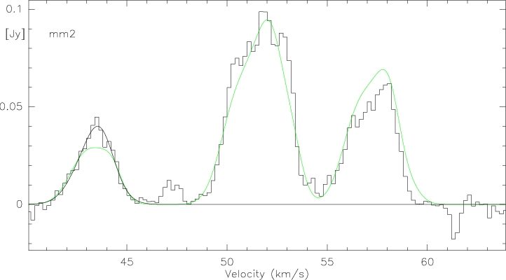
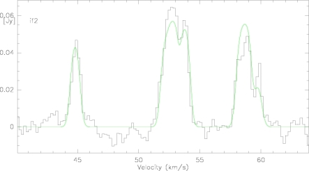
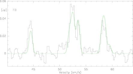
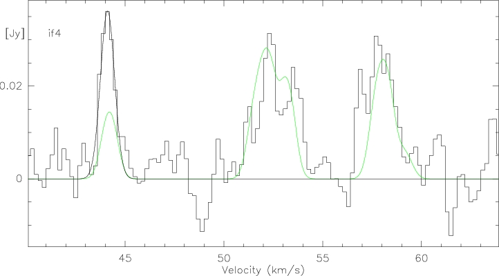
Figure 10: N₂H${}^{+}(1-0)$ spectra around 50 km s^-1 toward mm2 and the four interface positions if1 to if4. The green lines show N₂H⁺ fits taking into account the whole hyperfine structure whereas the black lines show two- and one-component Gaussian fits to the isolated hyperfine structure line $-8.0$ km s^-1 from the central peak. Peak velocities and line widths the hyperfine structure fits if1 to if3 and of the Gaussian fits (corrected for the $-8.0$ km s^-1 offset) for mm2 and if4 are presented in Table 3.

To further investigate the velocity sub-structure of the different components, we extracted N₂H${}^{+}(1-0)$ spectra toward mm1a, mm1b, mm2 and four positions in the interface region directly west of mm1 (see Fig. 8 for the four selected interface positions if1 to if4). Figures 9 and 10 show the corresponding 100 and 50 km s^-1 spectra at the different positions. At the positions of mm1a, mm1b and mm2, the optical depth is so high that no useful fits to the whole hyperfine structure was possible. For these positions, we extracted the peak velocities and line widths from Gaussian fits to the isolated hyperfine structure component $-8.0$ km s^-1 offset from the main peak. The spectrum toward if4 has an unusually strong isolated hyperfine structure component that the hyperfine fitting was difficult as well. Therefore, here we also use the fit results from the Gaussian fit to the isolated hyperfine structure component. For the other three interface positions if1 to if3, fitting the whole hyperfine structure worked reasonably well. Table 3 presents the derived peak velocities and line widths.

Table 3: Parameters of N₂H⁺(1–0) emission peaks

	$v$	$\Delta v$	$M_{\rm{vir}}$
	km/s	km/s	M⊙
mm1a	100.2	1.2	8.7-13.1
mm1a	101.6	1.0	6.0-9.1
mm1b	100.6	1.1	7.3-11.0
mm1b	101.6	0.8	3.9-5.8
mm2	51.3	2.2	29.3-44.1
mm2	51.8	1.5	13.6-20.5
if1	52.6	0.8	3.9-5.8
if2	52.8	0.7	3.0-4.5
if3	52.5	0.7	3.0-4.5
if4	52.1	0.8	3.9-5.8

For mm1a, mm1b, mm2 and if4, the fits results from the Gaussian fits to the isolated hyperfine structure line (corrected for the $-8.0$ km s^-1 offset) are presented. For if1 to if3, the corresponding results from the whole hyperfine structure line fits are listed.

Independent of being part of two very different general velocity components at 100 and 50 km s^-1, the mm peak positions mm1a, mm1b and mm2 all three show double peaked N₂H${}^{+}(1-0)$ emission where the spectral peaks are separated between 0.5 and 1.4 km s^-1 (Table 3). It is interesting to note that Beuther & Henning (2009) found also double-peaked N₂H⁺ spectra within the IRDC 19175 region, and recently Ragan et al. (in prep.) identified similar signatures in a mid-infrared dark clump of the Snake IRDC G11.11. Ragan et al. (in prep.) will discuss this effect in more detail.

The N₂H⁺ line widths $\Delta v$ on the order of 1 km s^-1 are larger than the thermal line width at 15 K of $\sim$0.15 km s^-1. However, since our spectral resolution is only 0.2 km s^-1 we could not even resolve much narrower lines properly. Therefore, our measured line width have to be considered as upper limits, and the actual line widths for some cores may in fact not be too far off from pure thermal line widths. In contrast to the luminosities, where we find considerable differences between different regions (see section luminous for a discussion), the observed N₂H⁺ line widths of several different IRDCs is very similar (e.g., IRDC 18223-3, IRDC 19175, Beuther et al. 2005b; Beuther & Henning 2009).

Following MacLaren et al. (1988), we calculated the virial masses $M_{\rm{vir}}=k_{2}\times R\times\Delta v^{2}$ with the constant $k_{2}$ between 190 and 126 for $1/r$ or $1/r^{2}$ density distributions, the core radius $R$ (in units of parsecs) and the N₂H⁺(1–0) line width $\Delta v$. For the radius we assumed all sources to be unresolved with an average N₂H⁺(1–0) synthesized beam of $\sim 3.6^{\prime\prime}$, corresponding to the core diameter of 19800 AU. Table 3 lists the range of virial masses for the given line widths and assumed density distributions. Interestingly, the gas masses derived for mm1a and mm1b from the 3.23 mm continuum data (Table 2) are a factor of a few larger than the virial masses estimated from the N₂H⁺ data. While mass estimates from the dust continuum emission as well as virial masses both have notoriously large errors on the order of a few, nevertheless, the data from mm1a and mm1b are consistent with starless massive gas cores that are likely gravitationally bound and may collapse and form stars in the near future.

4 Discussion

4.1 Luminous starless clumps

The measured high luminosities from the starless clump candidates (Fig.3), in particular clumps 1, 3 and 8a are intriguing since – down to our detection limits – they do not have an internal radiation sources. Also other sources like clump 2 are interesting because this region is still dark at 24 $\mu$m and only becomes an emission source from 70 $\mu$m onwards. Hence, it has to be at a very young evolutionary stage as well. This implies that the bolometric luminosities of these regions must be largely caused by external radiation sources of which the prime candidates are the diverse sources comprising the neighboring mini-starburst W43 (see Introduction or, e.g., Motte et al. 2003; Nguyen Luong et al. 2011). Do we find differences between IRDCs in the vicinity of very active massive star-forming regions and more isolated IRDCs?

For comparison, we select the IRDC 18223 where luminosities and temperatures were measured in a similar fashion via SED fits of Herschel data (Beuther et al., 2010). The derived temperatures for the clumps in IRDC 18454 are slightly elevated compared to IRDC 18223 (between 19 and 20 K for IRDC 18454, and between 16 and 18 K in IRDC 18223), and the measured bolometric luminosities in IRDC 18454 are factors between 4 and 10 larger than found in IRDC 18223. While the observed aperture size and spatial scale directly translates into different luminosities (Fig. 3), the smaller aperture of $19.2^{\prime\prime}$ (corresponding to $\sim$0.5 pc) used for IRDC 18454 is even smaller than that used for IRDC 18223 ($\sim$0.64 pc). Therefore, spatial scale arguments cannot account for that difference. Another important parameter for the total bolometric luminosity is the available gas mass. While clumps 1 and 3 are factors of a few more massive than IRDC 18223-s1 and IRDC 18223-s2, clump 8 presented here and IRDC 18223-s2 have approximately the same mass (140 and 170 M_⊙, respectively). Nevertheless, the luminosity of clump 8 is about a factor 4 larger than that of IRDC 18223-s2. It is no surprise that the temperature differences between IRDC 18223 and IRDC 18454 are less strong than the luminosity differences because the luminosity has a strong exponential dependence on the temperature (Stefan-Boltzmann law $L\propto T^{4}$).

While all these parameters have to be taken a bit cautiously since the associated errors are large (e.g., for the SEDs the uncertain background subtraction may contribute significantly), in principle the errors should be comparable for the different regions because we applied the same techniques. Therefore, it is tempting to speculate what may cause the measured luminosity and temperature differences between infrared dark clumps in the vicinity of the active star-forming region W43 compared to the more quiescent region IRDC 18223. It could be possible that the neighboring mini-starburst injects considerable energy even into the starless clumps that the total bolometric luminosities are increased above their expected more quiescent values. To first order, with such a luminosity increase one also expects a temperature increase within the gas clumps. Although the measured temperature difference between the regions is less strong than the luminosity increase, nevertheless, we see elevated temperatures in IRDC 18454 compared to IRDC 18223. Considering the large apertures used for the SEDs, the derived average temperatures may still be dominated by the average temperature of the general ISM that is in the same range (e.g., Reach et al. 1995).

We can also quantitatively estimate the influence of the total bolometric luminosity of the Wolf-Rayet/OB cluster ($\sim 3.5\times 10^{6}$ L_⊙) on the gas and dust environment at the typical projected separations from the target IRDCs (Fig. 1). Assuming that all radiation of the central cluster is reprocessed as far-infrared radiation, and using an approximate projected separation of the infrared dark clumps of 11 pc, as well as Gaussian source FWHM of $36.6^{\prime\prime}$ or $19.2^{\prime\prime}$, respectively (Sec. 3.2 and Fig. 3), the received luminosity at the location of the IRDCs are on the order of 2500 and 700 L_⊙, respectively. Comparing these values with the measured luminosities in the same given apertures (Fig. 3), elevated luminosities caused by the nearby luminous cluster appear clearly feasible. Furthermore, one can estimate the approximate required interstallar radiation field to account for the observed luminosity. A clump with a surface corresponding to a radius $19.2^{\prime\prime}/2$ has to intercept an interstellar radiation field of $\sim$306 (in units of the Habing field $G_{0}=1.6\times 10^{-3}$ erg s^-1cm^-2, Habing 1968) to exhibit a luminoisty of 1000 L_⊙. In comparison, if one just accounts for geometric dillution, the $\sim 3.5\times 10^{6}$ L_⊙ of the Wolf-Rayet/OB cluster correspond at a distance of 11 pc to $\sim$588 times the interstellar radiation field. Subtracting additional scattering and blockade by interfering gas clumps, these two values agree well with each other. Based on kinematic arguments, Motte et al. (2003) also discussed the influence of the luminous cluster on the environment, and they similarly infer that there should be considerable influence from that first generation of high-mass star formation on its environment.

In addition to the individual SED fits presented in section 3.2 and Figure 3, one can also smooth all maps between 70 and 870 $\mu$m to the same spatial resolution of the 500 $\mu$m data and fit the SEDs pixel by pixel (see also Stutz et al. 2010 for details of the fitting). This large-scale fitting approach allows us to infer the dust temperature structure and gradients across the whole field. Figure 11 presents the results. As expected, we identify a clear temperature gradient from more than 35 K toward the W43 main complex down to low values below 20 K in the east of the region. In particular, we see that many of the submm continuum structures correlate well with the lowest temperatures. This is true for the dark clumps of this analysis as well as for the filament going approximately in northsouth direction at the eastern edge of the map. The large-scale east-west temperature gradient throughout the region is consistent with significant influence of the W43 complex on the here discussed infrared dark high-mass starless clump candidates.

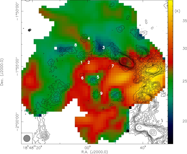
Figure 11: The color-scale shows a temperature map in K derived for the whole region from the combined Herschel and ATLASGAL data between 70 and 870 $\mu$m, all smoothed to the spatial resolution of the 500 $\mu$m data. Contour levels of the overlaid 870 $\mu$m data start at the 3$\sigma$ levels of 0.27 mJy beam^-1 and continue in in 3$\sigma$ steps to 2.7 Jy beam^-1, from where they continue in 2.7 Jy beam^-1 steps. Our target clumps are marked.

Since the Jeans length and Jeans mass as indicators of the fragmentation properties of star-forming gas clumps are proportional to the temperature ($\lambda_{J}\propto T^{1/2}$ and $M_{J}\propto M^{3/2}$), increases in luminosity and temperature of young gas clumps could change their fragmentation properties to preferentially form larger and more massive fragments. Although still speculative, such a scenario could imply that nearby active star formation does not only have a destructive character destroying pristine gas clumps, but that the energy input of close-by active regions could even elevate the ability to form massive stars in a triggered fashion in the immediate environment of the earlier generations of stars. While the energy input from a first generation of low-mass stars appears to be too little to halt fragmentation (Longmore et al., 2011), the influence of the nearby luminous high-mass star-forming region may be more important.

4.2 Colliding clouds or chance alignment?

As indicated in sections 3.3 & 3.4.2, the two different velocity components at 100 and 50 km s^-1 may either be chance projections along the line of sight, or they could be associated and potentially interacting cloud complexes. Based mainly on large-scale ¹³CO(1–0) data from the Galactic Ring survey (GRS, Jackson et al. 2006), Nguyen Luong et al. (2011) suggest that the velocities associated directly with W43 range between 60 and 120 km s^-1, whereas lower velocity components are unlikely part of the W43 complex.

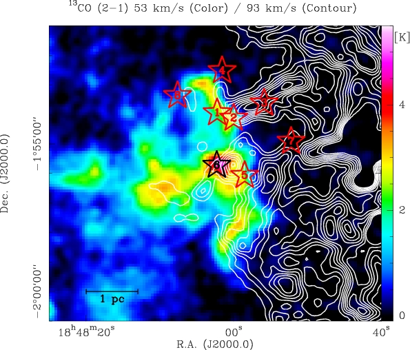
Figure 12: IRAM 30m ¹³CO(2–1) observations toward a larger part of W43 and IRDC 18454. The color-scale shows the ¹³CO emission around 53 km s^-1 whereas the contours present gas at 93 km s^-1. The stars mark the positions of our clumps 1 to 8, a scale-bar is shown at the bottom-left.

In contrast to this, the spatial structure of the two velocity components as presented in Figs. 4 and 6 indicates that the two components may also be spatially associated and interacting. Also the fact that the mm fluxes of clump 1 and 2 are so similar could be taken as circumstantial support for this idea.

To further investigate whether we find additional signatures of associated clouds in that region, we investigated the ¹³CO(2–1) data of a recent IRAM 30 m large program to study the entire W43 complex (PI F. Motte). The whole project, the data and more detailed analysis will be presented in forthcoming papers by Nguyen-Luong et al. and Carlhoff et al., here we only show a small sub-set where two selected velocity components are compared. Figure 12 presents an overlay of the ¹³CO(2–1) emission around 50 and 100 km s^-1 over a larger area but also encompassing our region of interest. The two velocity components appear in projection as a layered structure where one velocity component mainly emits at locations that are devoid of emission from the other velocity component. Unfortunately, this is also no unambiguous proof for associated or interacting clouds. However, the spatial alignment of different velocity components for molecules with varying critical densities over a broad range of spatial scales is suggestive for the idea of connected and interacting structures.

Additional interesting information about different velocity components in this region is found for other tracers and wavelengths as well. For example, CH₃OH Class ii maser were found in this region at both velocities (e.g., Menten 1991). Furthermore, the recent Hii region radio recombination line survey of Anderson et al. (2011) detected toward 21 out of 23 targeted position within 0.5 degrees from W43 two velocity components as well (one of the positions is marked in Fig. 1). While projection effects of molecular and atomic gas along the line of sight through the Galaxy are well known, having such a large number of multiple-velocity recombination line spectra is more surprising since one does not expect that many projected Hii regions along each line of sight. Hence interacting clouds and Hii regions are possible. Furthermore, it is interesting to note that the largest number of Hii regions in our Galaxy are also found toward Galactic longitudes around $l\approx\pm 30$ degrees (Wilson et al., 1970; Lockman, 1979; Anderson et al., 2011), hence again including the W43/IRDC 18454 complex. All this evidence suggests special environmental physical properties in this region that may affect the star formation processes.

How could such interacting velocity components be explained? The whole W43-IRDC 18454 complex is located at approximately a Galactic longitude of 30.85 degrees where the Galactic bar ends and the Scutum spiral arm starts (for a recent description of the different Galactic components, see e.g., Churchwell et al. 2009; Nguyen Luong et al. 2011). Hence, one could fathom interaction between Galactic bar and spiral arm structures, e.g., streaming motions between both Galactic components. Following the Galaxy modeling by Bissantz et al. (2003), the inner spiral arms connecting to the bar and the bar should co-rotate. In this framework, the 100 km s^-1 component should be associated with the beginning of the Scutum arm (see also Vallée 2008). Spiral arm velocities for the Sagittarius and Perseus arm are, according to Vallée (2008), around 70 and 25 km s^-1, respectively. However, there is no clear association with a 50 km s^-1 gas component. Inspecting the Galactic plane CO survey by Dame et al. (2001), at a Galactic longitude of $\sim 30.85$ degrees one also find strong emission at 100 km s^-1 and only less prominent features at 50 km s^-1. Therefore, from the spiral arm structure of our Galaxy, it is not obvious to what distance one can associate the 50 km s^-1 component. Furthermore, Nguyen Luong et al. (2011) associate even 60 km s^-1 gas with W43 and not so much with the Sagittarius arm as one would expect from the Galaxy models (e.g., Vallée 2008). Although we cannot firmly establish whether the 100 and 50 km s^-1 gas components are spatially associated or just chance alignments, the close projected association of them as well as the extremely busy and active nature of that part of the Galaxy at the interface of the Galactic bar with the inner spiral arm, where streaming motions between both components are likely to occur, makes spatial association and interaction of different cloud components here a fair possibility. See also Anderson et al. (2011) for a similar discussion of the origin of the ionized gas.

One way to distinguish the different explanation is to derive accurate distances to the different components. And the best way to do that today is parallax measurements of maser sources (e.g., Reid et al. 2009). The VLBI now has a very large project to do that for many maser sources throughout the Galactic plane (PI M. Reid), and the masers toward the W43 complex are part of that program (K. Menten, priv. comm.). Therefore, we expect to get accurate distances for the different velocity components in the coming years. That should then allow us to answer the question whether these different velocity components are indeed spatially associated or whether they are just chance projections along the lines of sight.

5 Conclusions

The W43 complex is know as one of the most active sites of star formation in our Galaxy. Our aim in that context was to investigate the nature of very young massive gas clumps in the vicinity of W43 prior to star formation or at very early evolutionary stages. A multi-wavelength continuum study of the region between 70 $\mu$m and 1.2 mm wavelengths allows us to isolate gas clumps that are still dark at 70 $\mu$m wavelengths. These are among the best candidates of being genuine high-mass starless cores. An analysis of the spectral energy distributions finds temperatures between 19 and 21 K and luminosities usually larger than 1000 L_⊙ for these high-mass starless clump candidates. These values are larger than those found toward infrared dark clouds in more quiescent environments. A clear temperature gradient from the luminous W43 complex to the studied starless clump candidates is identified. We discuss whether the nearby mini-starburst W43 not only has destructive effects on nearby gas clumps, but that elevating the average gas temperatures can increase the Jeans length and Jeans mass, hence favoring the formation of massive stars in the environment.

An analysis of the spectral data obtained with single-dish instruments and the Plateau de Bure interferometer reveals two different velocity components at 100 and 50 km s^-1. While chance projection along the line of sight is possible, the projected spatial association of the two gas components indicates that the two components may be spatially associated or even interacting. We discuss the general velocities expected in that part of our Galaxy. While the 100 km s^-1 component associated also with W43 appears to be clearly part of the Scutum arm that starts at the end of the inner Galactic bar, it is more difficult to clearly associate the 50 km s^-1 with a distinct Galactic feature. Therefore, it remains possible that the extremely active location of that region at the interface of the Galactic bar and the inner spiral arm hosts clouds at different velocities that may be interacting.

References

- Anderson et al. (2011) Anderson, L. D., Bania, T. M., Balser, D. S., & Rood, R. T. 2011, ApJS, 194, 32
- Bally et al. (2010) Bally, J., Anderson, L. D., Battersby, C., et al. 2010, A&A, 518, L90
- Battersby et al. (2011) Battersby, C., Bally, J., Ginsburg, A., et al. 2011, ArXiv e-prints
- Benjamin et al. (2005) Benjamin, R. A., Churchwell, E., Babler, B. L., et al. 2005, ApJ, 630, L149
- Bergin & Tafalla (2007) Bergin, E. A. & Tafalla, M. 2007, ARA&A, 45, 339
- Beuther et al. (2007) Beuther, H., Churchwell, E. B., McKee, C. F., & Tan, J. C. 2007, in Protostars and Planets V, ed. B. Reipurth, D. Jewitt, & K. Keil, 165–180
- Beuther & Henning (2009) Beuther, H. & Henning, T. 2009, A&A, 503, 859
- Beuther et al. (2010) Beuther, H., Henning, T., Linz, H., et al. 2010, A&A, 518, L78
- Beuther et al. (2002) Beuther, H., Schilke, P., Menten, K. M., et al. 2002, ApJ, 566, 945
- Beuther et al. (2005a) Beuther, H., Schilke, P., Menten, K. M., et al. 2005a, ApJ, 633, 535
- Beuther & Sridharan (2007) Beuther, H. & Sridharan, T. K. 2007, ApJ, 668, 348
- Beuther et al. (2005b) Beuther, H., Sridharan, T. K., & Saito, M. 2005b, ApJ, 634, L185
- Beuther & Steinacker (2007) Beuther, H. & Steinacker, J. 2007, ApJ, 656, L85
- Bissantz et al. (2003) Bissantz, N., Englmaier, P., & Gerhard, O. 2003, MNRAS, 340, 949
- Blum et al. (1999) Blum, R. D., Damineli, A., & Conti, P. S. 1999, AJ, 117, 1392
- Brand & Blitz (1993) Brand, J. & Blitz, L. 1993, A&A, 275, 67
- Carey et al. (2000) Carey, S. J., Feldman, P. A., Redman, R. O., et al. 2000, ApJ, 543, L157
- Carey et al. (2009) Carey, S. J., Noriega-Crespo, A., Mizuno, D. R., et al. 2009, PASP, 121, 76
- Churchwell et al. (2009) Churchwell, E., Babler, B. L., Meade, M. R., et al. 2009, PASP, 121, 213
- Cyganowski et al. (2008) Cyganowski, C. J., Whitney, B. A., Holden, E., et al. 2008, AJ, 136, 2391
- Dame et al. (2001) Dame, T. M., Hartmann, D., & Thaddeus, P. 2001, ApJ, 547, 792
- Draine et al. (2007) Draine, B. T., Dale, D. A., Bendo, G., et al. 2007, ApJ, 663, 866
- Egan et al. (1998) Egan, M. P., Shipman, R. F., Price, S. D., et al. 1998, ApJ, 494, L199
- Elia et al. (2010) Elia, D., Schisano, E., Molinari, S., et al. 2010, A&A, 518, L97
- Griffin et al. (2010) Griffin, M. J., Abergel, A., Abreu, A., et al. 2010, A&A, 518, L3
- Habing (1968) Habing, H. J. 1968, Bull. Astron. Inst. Netherlands, 19, 421
- Henning et al. (2010) Henning, T., Linz, H., Krause, O., et al. 2010, A&A, 518, L95
- Hildebrand (1983) Hildebrand, R. H. 1983, QJRAS, 24, 267
- Jackson et al. (2006) Jackson, J. M., Rathborne, J. M., Shah, R. Y., et al. 2006, ApJS, 163, 145
- Kroupa (2001) Kroupa, P. 2001, MNRAS, 322, 231
- Krumholz & McKee (2008) Krumholz, M. R. & McKee, C. F. 2008, Nature, 451, 1082
- Kurtz et al. (1994) Kurtz, S., Churchwell, E., & Wood, D. O. S. 1994, ApJS, 91, 659
- Lester et al. (1985) Lester, D. F., Dinerstein, H. L., Werner, M. W., et al. 1985, ApJ, 296, 565
- Linz et al. (2010) Linz, H., Krause, O., Beuther, H., et al. 2010, A&A, 518, L123
- Liszt et al. (1993) Liszt, H. S., Braun, R., & Greisen, E. W. 1993, AJ, 106, 2349
- Lockman (1979) Lockman, F. J. 1979, ApJ, 232, 761
- Longmore et al. (2011) Longmore, S. N., Pillai, T., Keto, E., Zhang, Q., & Qiu, K. 2011, ApJ, 726, 97
- López-Corredoira et al. (2007) López-Corredoira, M., Cabrera-Lavers, A., Mahoney, T. J., et al. 2007, AJ, 133, 154
- MacLaren et al. (1988) MacLaren, I., Richardson, K. M., & Wolfendale, A. W. 1988, ApJ, 333, 821
- Mathis et al. (1977) Mathis, J. S., Rumpl, W., & Nordsieck, K. H. 1977, ApJ, 217, 425
- Menten (1991) Menten, K. 1991, in Astronomical Society of the Pacific Conference Series, 119
- Molinari et al. (1996) Molinari, S., Brand, J., Cesaroni, R., & Palla, F. 1996, A&A, 308, 573
- Molinari et al. (2010) Molinari, S., Swinyard, B., Bally, J., et al. 2010, A&A, 518, L100
- Motte et al. (2007) Motte, F., Bontemps, S., Schilke, P., et al. 2007, A&A, 476, 1243
- Motte et al. (2003) Motte, F., Schilke, P., & Lis, D. C. 2003, ApJ, 582, 277
- Motte et al. (2010) Motte, F., Zavagno, A., Bontemps, S., et al. 2010, A&A, 518, L77+
- Negueruela et al. (2011) Negueruela, I., González-Fernández, C., Marco, A., & Clark, J. S. 2011, A&A, 528, A59+
- Nguyen Luong et al. (2011) Nguyen Luong, Q., Motte, F., Schuller, F., et al. 2011, A&A, 529, A41
- Ossenkopf & Henning (1994) Ossenkopf, V. & Henning, T. 1994, A&A, 291, 943
- Ott (2010) Ott, S. 2010, in Astronomical Society of the Pacific Conference Series, Vol. 434, Astronomical Data Analysis Software and Systems XIX, ed. Y. Mizumoto, K.-I. Morita, & M. Ohishi, 139–+
- Perault et al. (1996) Perault, M., Omont, A., Simon, G., et al. 1996, A&A, 315, L165
- Peretto & Fuller (2009) Peretto, N. & Fuller, G. A. 2009, A&A, 505, 405
- Pilbratt et al. (2010) Pilbratt, G. L., Riedinger, J. R., Passvogel, T., et al. 2010, A&A, 518, L1
- Poglitsch et al. (2010) Poglitsch, A., Waelkens, C., Geis, N., et al. 2010, A&A, 518, L2
- Rathborne et al. (2006) Rathborne, J. M., Jackson, J. M., & Simon, R. 2006, ApJ, 641, 389
- Reach et al. (1995) Reach, W. T., Dwek, E., Fixsen, D. J., et al. 1995, ApJ, 451, 188
- Reid et al. (2009) Reid, M. J., Menten, K. M., Zheng, X. W., et al. 2009, ApJ, 700, 137
- Rodriguez-Fernandez & Combes (2008) Rodriguez-Fernandez, N. J. & Combes, F. 2008, A&A, 489, 115
- Sawada et al. (2008) Sawada, T., Ikeda, N., Sunada, K., et al. 2008, PASJ, 60, 445
- Schuller et al. (2009) Schuller, F., Menten, K. M., Contreras, Y., et al. 2009, A&A, 504, 415
- Simon et al. (2006) Simon, R., Jackson, J. M., Rathborne, J. M., & Chambers, E. T. 2006, ApJ, 639, 227
- Smith et al. (1978) Smith, L. F., Biermann, P., & Mezger, P. G. 1978, A&A, 66, 65
- Sridharan et al. (2005) Sridharan, T. K., Beuther, H., Saito, M., Wyrowski, F., & Schilke, P. 2005, ApJ, 634, L57
- Sridharan et al. (2002) Sridharan, T. K., Beuther, H., Schilke, P., Menten, K. M., & Wyrowski, F. 2002, ApJ, 566, 931
- Stutz et al. (2010) Stutz, A., Launhardt, R., Linz, H., et al. 2010, A&A, 518, L87
- Vallée (2008) Vallée, J. P. 2008, AJ, 135, 1301
- Williams et al. (2000) Williams, J. P., Blitz, L., & McKee, C. F. 2000, Protostars and Planets IV, 97
- Wilson et al. (1970) Wilson, T. L., Mezger, P. G., Gardner, F. F., & Milne, D. K. 1970, A&A, 6, 364
- Wood & Churchwell (1989a) Wood, D. O. S. & Churchwell, E. 1989a, ApJ, 340, 265
- Wood & Churchwell (1989b) Wood, D. O. S. & Churchwell, E. 1989b, ApJS, 69, 831